Taisuke Otsu and Yoshiyasu Rai
Bootstrap inference of matching estimators for
average treatment effects
Article (Accepted version)
(Refereed)
Original citation:
Otsu, Taisuke and Rai, Yoshiyasu (2016) Bootstrap inference of matching estimators for average treatment effects. Journal of the American Statistical Association ISSN 0162-1459 DOI: 10.1080/01621459.2016.1231613
© 2017 Taylor & Francis
This version available at: http://eprints.lse.ac.uk/84170/ Available in LSE Research Online: September 2017
LSE has developed LSE Research Online so that users may access research output of the School. Copyright © and Moral Rights for the papers on this site are retained by the individual authors and/or other copyright owners. Users may download and/or print one copy of any article(s) in LSE Research Online to facilitate their private study or for non-commercial research. You may not engage in further distribution of the material or use it for any profit-making activities or any commercial gain. You may freely distribute the URL (http://eprints.lse.ac.uk) of the LSE Research Online website.
This document is the author’s final accepted version of the journal article. There may be differences between this version and the published version. You are advised to consult the publisher’s version if you wish to cite from it.
BOOTSTRAP INFERENCE OF MATCHING ESTIMATORS FOR AVERAGE TREATMENT EFFECTS
TAISUKE OTSU AND YOSHIYASU RAI
Abstract. Abadie and Imbens (2008) showed that the naive bootstrap is not
asymp-totically valid for a matching estimator of the average treatment effect with a fixed number of matches. In this article, we propose asymptotically valid inference meth-ods for matching estimators based on the weighted bootstrap. The key is to construct bootstrap counterparts by resampling based on certain linear forms of the estimators. Our weighted bootstrap is applicable for the matching estimators of both the average treatment effect and its counterpart for the treated population. Also, by incorporating a bias correction method in Abadie and Imbens (2011), our method can be asymptotically valid even for matching based on a vector of covariates. A simulation study indicates that the weighted bootstrap method is favorably comparable with the asymptotic normal approximation by Abadie and Imbens (2006). As an empirical illustration, we apply the proposed method to the National Supported Work data.
1. Introduction
The method of matching is widely applied in empirical research for treatment effects and program evaluations. In a series of papers, Abadie and Imbens (2006, 2008, 2011, 2012) studied various aspects of matching estimators for average treatment effects with fixed numbers of matches. In contrast to other studies on nonparametric estimation of treatment effects (e.g., Heckman, Ichimura and Todd, 1998, and Hirano, Imbens and Rid-der, 2003), Abadie and Imbens analyzed rather nonstandard behaviors of the matching
We thank Joachim Freyberger, Jack Porter, Xiaoxia Shi and Christopher Taber for thoughtful comments. We also thank Martin Huber for a computer program. We acknowledge substantial comments from an anonymous referee regarding the general weighted bootstrap scheme. Financial support from the ERC Consolidator Grant (SES-0720961) is gratefully acknowledged (Otsu).
estimators due to lack of smoothness of the functional forms caused by the fixed numbers
of matches. Abadie and Imbens (2006) showed that the matching estimators are not√N
-consistent in general, where N is the sample size. Abadie and Imbens (2011) proposed a
bias correction method based on nonparametric series regression. In addition to the non-standard asymptotic behavior of the point estimator, Abadie and Imbens (2008) provided an example to show that the standard naive bootstrap (i.e., resampling from observations with equal weights) fails to provide an asymptotically valid standard error and quantiles for a matching estimator. As Abadie and Imbens (2008) argued, the main reason for this failure is that the naive bootstrap fails to reproduce the distribution of the number of
times each unit is used as a match.1 Given this negative result on the bootstrap, Abadie
and Imbens (2008) recommended using the asymptotic standard error derived in Abadie and Imbens (2006) or subsampling (Politis and Romano, 1994) for inference.
In this paper, we propose an alternative inference method for the matching estimators based on the weighted bootstrap (e.g., Mason and Newton, 1992, and Pauly, 2011). We show that even though the naive bootstrap is not valid for the matching estimator, the weighted bootstrap approach based on a linear form of the estimator can still be valid for inference based on the estimator. The intuition for the validity of our weighted bootstrap
is that we treat the number of times unitiis used for a match (i.e.,KM(i)defined in (2.1))
as one of the characteristics of unit i and directly resample it. Such resampling preserves
the distribution of KM(i)in bootstrap resamples and circumvents the problem in Abadie
and Imbens (2008). The weights for bootstrapping are flexible: they can be multinomial, Dirichlet (as in the Bayesian bootstrap by Rudin, 1981), or some two-point distribution (as in the wild bootstrap by Mammen, 1993). We note that the weighted bootstrap using multinomial weights (which resamples from the linear form of the estimator) is
1Denoted byK
M(i) in (2.1) below. It means how many times uniti’s observation appears to estimate potential outcomes by imputations.
different from the naive bootstrap (which resamples from the original data). Indeed, Abadie and Imbens (2008, p. 1546) mentioned the possibility of using the wild bootstrap for valid inference. As a special case, this paper formally confirms their conjecture. Also, Abadie and Imbens (2012) provided a representation of the matching estimator based on
a martingale sequence of length 2N. We argue that although it is possible to conduct
the weighted bootstrap based on this martingale representation (where we draw weights
of size 2N), it is indeed enough to resample from the linear form of the estimator (where
we draw weights of only size N).
We show the asymptotic validity of the weighted bootstrap for both the average treat-ment effect and its counterpart on the treated population. Also, by incorporating a bias correction method in Abadie and Imbens (2011), our method can be asymptotically valid even for matching based on a vector of covariates. A small simulation study indicates that our weighted bootstrap method is favorably comparable with the asymptotic normal approximation by Abadie and Imbens (2006). Finally, the proposed method is illustrated by an empirical analysis using the National Supported Work data.
The paper is organized as follows. Section 2 introduces our basic setup and notation. In Section 3, we present the weighted bootstrap method and show its asymptotic validity. Section 4 presents some simulation results. In Section 5, we apply the weighted bootstrap method to the National Supported Work data. Section 6 concludes. In Appendix A, we list assumptions for the main theorem and provide some remarks. All proofs are contained in Appendices B and C. Tables are presented in Appendix D. In the web appendix, we present an analogous result of bootstrap validity for the case of the average treatment effect on the treated population and sketch how our weighted bootstrap approach may be applied to the average derivative estimator under the small bandwidth asymptotics of Cattaneo, Crump and Jansson (2010, 2014).
2. Setup
Let us introduce the basic setup. For each unit i= 1, . . . , N, we observe an indicator
variable Di for a treatment (Di = 1 if treated and Di = 0 otherwise), and outcome
Yi = Yi(0) if Di = 0 Yi(1) if Di = 1 ,
where Yi(0) and Yi(1) are potential outcomes for Di = 0 and 1, respectively. Also we
observe a vector of covariates Xi for each unit. Based on the non-experimental
obser-vations {Yi, Di, Xi}Ni=1 of size N, we wish to conduct inference on the average treatment
effect τ = E[Yi(1)−Yi(0)]. Let I{A} be the indicator function for an event A and kxk
be the Euclidean norm. To estimate τ, we consider the matching estimator based on the
distance measured by the covariates,
ˆ τ = 1 N N X i=1 {Yˆi(1)−Yˆi(0)},
where Yˆi(0) and Yˆi(1) are estimates of the potential outcomes by imputations defined as
ˆ Yi(0) = Yi if Di = 0, 1 M P j∈JM(i)Yj if Di = 1, ˆ Yi(1) = 1 M P j∈JM(i)Yj if Di = 0, Yi if Di = 1,
and JM(i)is the set of indices of the first M matches for unit i,
JM(i) = ( j ∈ {1, . . . , N}:Dj = 1−Di, X l:Dl=1−Di I{kXl−Xik ≤ kXj−Xik} ≤M ) .
For the estimator τˆ, each unit may be used as a match more than once (matching with
Euclidean distance. Let KM(i) denote the number of times uniti is used as a match KM(i) = N X l=1 I{i∈ JM(l)}. (2.1)
In practice, it is common that the number of matches M can be small (could be one)
even though the sample size N is large. To characterize behaviors of the matching
es-timators in such a practical scenario, Abadie and Imbens (2006) analyzed asymptotic
properties of τˆas N increases to infinity with fixedM (called fixed-M asymptotics).
Let µ(d, x) = E[Y|D = d, X = x] and σ2(d, x) = V ar(Y|D = d, X = x). Note
that Assumption M (iii) in Appendix A guarantees µ(d, x) = E[Y(d)|X = x]. Under
Assumption M, Abadie and Imbens (2006, Theorems 3 and 4) showed thatτˆis consistent
and asymptotically normal, i.e.,
√
N(ˆτ−BN −τ) σN
d
→N(0,1), (2.2)
as N → ∞ (but M is fixed), where BN and σ2N are asymptotic bias and variance terms,
respectively, defined as BN = 1 N N X i=1 (2Di−1) 1 M X j∈JM(i) {µ(1−Di, Xi)−µ(1−Di, Xj)} , σN2 = σ12N +σ22, σ12N = 1 N N X i=1 1 +M−1KM(i) 2 σ2(Di, Xi), σ22 = E[{(µ(1, Xi)−µ(0, Xi))−τ}2]. (2.3)
In empirical applications, researchers typically choose a smallM even for large samples.
The fixed-M asymptotics in (2.2) provides a useful approximation for the distributions of
in (2.2) is the presence of the bias termBN that depends on M. As shown in Abadie and
Imbens (2006, Theorems 1 and 2), this bias term satisfies BN = Op(N−1/k), where k is
the dimension of X. Therefore, if k≥2, τˆis not √N-consistent for τ.
To deal with this problem, Abadie and Imbens (2011) estimated BN by
ˆ BN = 1 N N X i=1 (2Di−1) 1 M X j∈JM(i) {µˆ(1−Di, Xi)−µˆ(1−Di, Xj)} , (2.4)
where µˆ(d, x) is a nonparametric estimator of µ(d, x). Requirements on µˆ(d, x) are
pre-sented in Assumption R in Appendix A. Abadie and Imbens (2011, Theorem 2) employed
a series estimator for µˆ(d, x) and showed a remarkable result: √N( ˆBN −BN)
p
→ 0
un-der certain regularity conditions allowing X to be a vector.2 As clarified in Abadie and
Imbens (2011), this surprisingly fast convergence rate follows from the fact that BˆN
ba-sically estimates the contrast µ(d,x˙)−µ(d, x) with x˙ −x → 0. However, in contrast to
the number of matches M, the series length should increase to infinity to guarantee the
fast convergence rate.3 Due to the fast convergence property of BˆN, the bias corrected
estimator τ˜= ˆτ−BˆN satisfies
√
N(˜τ−τ)/σN d
→N(0,1)(Abadie and Imbens, 2011,
The-orem 2). Since the asymptotic variance σ2
N can be consistently estimated (see, Theorem
2More specifically, Abadie and Imbens (2011) proposed a power series regression estimator for µˆ(d, x) with k-dimensional x. For a vector of nonnegative integers λ = (λ1, . . . , λk), let |λ| = P
k
h=1λh and
xλ=Qk h=1x
λh
h , wherexh is the h-th element ofx. Define a series{λ(l)}
∞
l=1 for all distinct vectors of λ
such that |λ(l)| is nondecreasing. Based on this series, consider anL-vectorpL(x) = (xλ(1), . . . , xλ(L))0
of power functions ofx. The power series estimator ofµ(d, x)is given by
ˆ µ(d, x) =pL(x)0 X i:Di=d pL(Xi)pL(Xi)0 !− X i:Di=d pL(Xi)Yi,
ford∈ {0,1}andx∈X, where(·)−is a generalized inverse. Suppose thatµ(d, x)is infinitely differentiable at x ∈ X and that the series length L grows with the sample size N and satisfies L = O(Nv) with
v ∈ (0,min{2/(4k+ 3),2/(4k2−k)}). Then, as shown in Abadie and Imbens (2011, Theorem 2), the
power series estimator µˆ(d, x)satisfies Assumption R in Appendix A and achieves the fast convergence
√
N( ˆBN−BN) p
→0for the bias term.
3A major requirement on the choice of the series length is to achieve|µˆ(d,·)−µ(d,·)|
k−1=op(N−1/2+1/k) (the last condition of Assumption R in Appendix A). When the dimensionkofX is large, this condition typically requires more stringent smoothness on µ(d, x)in x. For example, Abadie and Imbens (2011, Theorem 2) imposed infinite differentiability of µ(d, x)in x.
6 of Abadie and Imbens, 2006), this asymptotic normality result on τ˜yields a confidence
interval for τ, which is valid under fixed-M asymptotics.
Alternatively, one may consider bootstrap inference based on some resampling scheme. However, Abadie and Imbens (2008) provided an example showing that the naive
boot-strap method (i.e., resampling from the observations{Yi, Di, Xi}Ni=1with uniform weights)
is not valid to estimate the standard error of a matching estimator under fixed-M
asymp-totics. This failure is due to the fact that the naive bootstrap is not able to reproduce
the distribution of KM(i) in (2.1), the number of times each unit is used as a match. To
the best of our knowledge, currently there is no valid bootstrap procedure to approximate
the distribution of √N(˜τ −τ) under fixed-M asymptotics. Indeed, Abadie and Imbens
(2008, p. 1546) conjectured that a wild bootstrap method may be asymptotically valid
because of the fact that τ˜can be written by some linear forms. In this paper, we confirm
and generalize their conjecture by developing a new weighted bootstrap method that is
valid under fixed-M asymptotics and contains the wild bootstrap as a special case.
3. Weighted Bootstrap
In this section, we present a valid bootstrap method for the bias corrected matching
estimator τ˜= ˆτ −BˆN under fixed-M asymptotics. By the definitions of τˆ and BˆN, and
the fact that µˆ(1−Di, Xj) = ˆµ(Dj, Xj)for j ∈ JM(i), the estimator τ˜ can be written as
a linear form ˜ τ = 1 N N X i=1 (2Di−1) {Yi−µˆ(1−Di, Xi)} − 1 M X j∈JM(i) {Yj−µˆ(1−Di, Xj)} = 1 N N X i=1 (2Di−1) Yi−µˆ(1−Di, Xi) +M−1KM(i){Yi−µˆ(Di, Xi)} ≡ 1 N N X i=1 ˜ τi, (3.1)
where KM(i) is defined in (2.1). Let eˆi =Yi −µˆ(Di, Xi) and ξˆi = (2Di −1){µˆ(Di, Xi)− ˆ
µ(1−Di, Xi)} −τ˜. Then we are able to write the i-th ‘residual’ as
˜
τi−τ˜= (2Di −1){1 +M−1KM(i)}eˆi+ ˆξi. (3.2)
This expression is insightful. If we consider the population counterpartsei =Yi−µ(Di, Xi)
andξi = (2Di−1){µ(Di, Xi)−µ(1−Di, Xi)}−τ ofeˆi andξˆi, respectively, then the variance
components σ2
1N and σ22 appearing in (2.3) can be written as
σ21N = V ar √1 N N X i=1 (2Di−1){1 +M−1KM(i)}ei D,X ! , σ22 = V ar √1 N N X i=1 ξi ! ,
respectively, where D = (D1, . . . , DN) and X = (X1, . . . , XN). This suggests that valid
bootstrap inference may be possible if we treat {τ˜i}Ni=1 like ‘observations’ and resample
them. Precisely speaking, we construct the weighted bootstrap counterpart of √N(˜τ−τ)
as follows √ N T∗ = N X i=1 Wi∗(˜τi−τ˜), (3.3) where {W∗
i}Ni=1 is a sequence of random variables satisfying Assumption W in Appendix
A. Assumption W is general enough to include several popular bootstrap methods. For
example, the nonparametric bootstrap (Efron, 1979) sets the weight as Wi∗ = Mi∗/√N,
where(M1∗, . . . , MN∗)is a multinomial random vector withN draws onN equal probability
cells. The Bayesian bootstrap (Rubin, 1981) sets the weight as Wi∗ = δi∗/√N, where
(δ1∗, . . . , δ∗N) is drawn from a Dirichlet distribution. The wild bootstrap (Wu, 1986, and
Mammen, 1993) sets the weight as Wi∗ = ∗i/√N, where {∗
with E[∗i] = 0 and E[∗2
i ] = 1.
4 It should be noted that the nonparametric bootstrap
with the weight Wi∗ = Mi∗/√N is different from the naive bootstrap (i.e., draw from
the original observations {Yi, Di, Xi}Ni=1 with equal weights) investigated by Abadie and
Imbens (2008). See Remark 2 below for a detailed discussion.
Our main theorem, asymptotic validity of the weighted bootstrap under fixed-M
asymp-totics, is presented as follows (see Appendices B and C for a proof).
Theorem. Under Assumptions M, W, and R in Appendix A,
sup r
|Pr{√N T∗ ≤r|Z} −Pr{√N(˜τ −τ)≤r}|→p 0,
as N → ∞ with fixed M.
Remarks. 1. This theorem says that the distribution of the bootstrap statistic√N T∗
consistently estimates that of the target object√N(˜τ−τ)under the Kolmogorov distance.
For example, let q∗α/2 and q∗1−α/2 be the (α/2)-th and (1−α/2)-th quantiles of T∗
respec-tively. These quantiles can be estimated by simulating T∗. Then based on this theorem,
the 100(1−α)% bootstrap confidence interval ofτ is obtained as [˜τ−q1∗−α/2,τ˜−q∗α/2]. In our simulation study below, we employ this confidence interval.
2. As we mentioned above, our bootstrap method allows the nonparametric bootstrap
weights (i.e., Wi∗ = Mi∗/√N with multinomial Mi∗) while Abadie and Imbens (2008)
showed failure of the naive bootstrap. This is not a contradiction because these methods
resample different objects. The naive bootstrap draws a resample {Y∗
i , D∗i, Xi∗}Ni=1 from
4In the simulation and empirical studies below, we employ Mammen’s (1993) two point distribution
∗i =
−(√5−1)/2 with probability (√5 + 1)/2√5 (√5 + 1)/2 with probability (√5−1)/2√5 .
the original observations {Yi, Di, Xi}Ni=1 and then computes the bootstrap counterpart ˜ τ∗ = 1 N N X i=1 (2D∗i −1) Yi∗−µˆ(1−D∗i, Xi∗) +M−1KM∗ (i){Yi∗−µˆ(D∗i, Xi∗)} .
Note thatKM∗ (i)is computed by the bootstrap resample. As argued by Abadie and Imbens
(2008), this approach causes a problem because in the naive bootstrap resample the same
unit may appear multiple times, which occurs with probability 0in the population. This
event affects the number of times unit iis used as a match. As a result, the distribution
of KM∗ (i)fails to approximate that ofKM(i), and the naive bootstrap counterpartτ˜∗ fails
to recover the distribution of τ˜.
In contrast, the nonparametric bootstrap with Wi∗ =Mi∗/√N treats KM(i) as one of
the characteristics of uniti. Indeed our bootstrap draws a resample from{Yi, Di, Xi, KM(i)}Ni=1
and then computes the bootstrap counterpart without recomputing KM(i). Thus, our
bootstrap circumvents the above problem.
3. An insightful paper by Abadie and Imbens (2012) pointed out that the (bias
cor-rected) matching estimators can be written as martingale sequences. For instance, con-sider the triangular array
ξN,i= 1 √ N(2Di−1){µ(Di, Xi)−µ(1−Di, Xi)} −τ for i= 1, . . . , N 1 √ N(2Di−1){1 +M −1K M(i)}(Yi−µ(Di, Xi)) fori=N + 1, . . . ,2N
and filtrationFN,` =σ{D1, . . . , D`, X1, . . . , X`}for`= 1, . . . , N andFN,` =σ{D,X, Y1, . . . , Y`−N}
for` =N+1, . . . ,2N. Abadie and Imbens (2012) argued thatnP`
i=1ξN,i,FN,`, `= 1, . . . ,2N
o
is a martingale sequence satisfying√N(ˆτ−BN−τ) =
P2N
i=1ξN,i, and that asymptotic
nor-mality of the estimator directly follows from the martingale central limit theorem. This
bootstrap statistic in (3.3) can be written as √N T∗ =PN
i=1W ∗
i( ˆξN,i+ ˆξN,N+i), whereξˆN,i
is an estimated counterpart of ξN,i. Also we are able to utilize the martingale structure
more directly by constructing a bootstrap statistic √NT˜∗ = P2N
i=1W ∗
i ξˆN,i. Basically the
same argument shows asymptotic validity of T˜∗.
4. Abadie and Imbens (2012) considered two other applications of the above martingale
representation approach, matching without replacements and hot-deck imputation. It is easy to modify our weighted bootstrap method for those applications.
5. Instead of the weighted bootstrap method described above, one may use
subsam-pling (Politis and Romano, 1994) as an alternative inference method. In our setting, the
subsampling confidence interval for τ can be obtained as follows.
(i): Compute τ˜, σˆN, µˆ(1, x), and µˆ(0, x) from the entire sample.
(ii): Draw subsamples{Y∗
i , D
∗
i, X
∗
i}Si=1 without replacement from the entire sample.
(iii): ComputeσˆS and the bias corrected estimatorτ˜S = ˆτS−BˆSfrom the subsample
drawn in (ii), where
ˆ BS = 1 S S X i=1 (2D∗i −1) 1 M X j∈J∗ M(i) {µˆ(1−D∗i, Xi∗)−µˆ(1−D∗i, Xj∗)} .
(iv): Repeat (ii)-(iii) for different subsamples and report [˜τ −p
S/NσˆNq1∗−α/2,τ˜−
p
S/NσˆNqα/∗ 2]as the100(1−α)% subsampling confidence interval, whereqα/∗ 2 and
q∗1−α/2 are the(α/2)-th and(1−α/2)-th quantiles of√S(˜τS−τ˜)/σˆS, respectively.
By Politis and Romano (1994), this subsampling confidence interval is asymptotically valid
under mild conditions if S → ∞ and S/N → 0 as N → ∞. In the special case where
the estimator τ˜ is √N-consistent without bias adjustment, we do not need to subtract
ˆ
BS. Thus, unlike our weighted bootstrap approach, the subsampling method does not
the choice of the size of subsamples S, which may be a difficult task. Our simulation
results below suggest the subsampling confidence interval is sensitive to the choice of S
when the sample size N is moderate. Also, we note that the computational cost of our
weighted bootstrap is significantly cheaper than that of subsampling (see, Section 4 for some example). This is because the weighted bootstrap does not require computation of matches in the bootstrap resamples.
6. As suggested by an Associate Editor, it is an interesting direction for future research
to see whether the basic idea of our bootstrap approach (i.e., resample properly linearized objects by the weighted bootstrap) can be applied to other contexts, where the naive bootstrap is invalid due to lack of asymptotic linearity. In the Web Appendix, we sketch and conjecture how our weighted bootstrap approach for matching estimators may be applied to the average derivative estimator under the small bandwidth asymptotics of Cattaneo, Crump and Jansson (2010, 2014).
4. Simulation
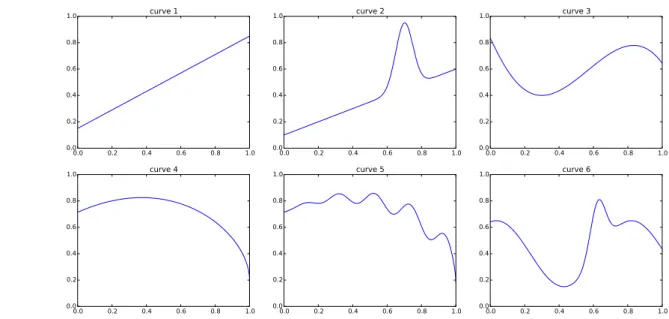
In this section, we evaluate the finite sample performance of our weighted bootstrap method by Monte Carlo simulation. Based on Frölich (2004) and Busso, DiNardo and
McCrary (2014), we consider the following data generating process for {Yi, Di, Xi}Ni=1,
Yi(1) = τ +m(kXik) +i, Yi(0) =m(kXik) +i, Di = I{P(Xi)≥νi}, νi ∼U[0,1],
P(Xi) = γ1+γ2kXik, Xi = (X1i, . . . , Xki)0,
Xji = ξi|ζji|/kζik for j = 1, . . . , k,
where(i, νi, ξi, ζi)are mutually independent. In this simulation design, the average
treat-ment effect is τ, which is set as τ = 0. For the parameters of P(Xi), we set γ1 = 0.15
and γ2 = 0.7.5 For the function m(·), we consider six curves presented in Table 1. For
k = dim(X), we considerk = 1,2, . . . ,5.
For all cases, we set the number of matches asM = 8,6 and consider the bias corrected
estimator τ˜ = ˆτ − BˆN, where BˆN is given by the OLS of the linear regression µˆi =
ˆ
α+Xiβˆ.7 We compare five inference methods: (i) wild bootstrap (weighted bootstrap
with Wi∗ = ∗i/√n, where ∗i is drawn from Mammen’s (1993) two point distribution),
(ii) nonparametric bootstrap (weighted bootstrap with Wi∗ = Mi∗/√n), (iii) asymptotic
t using Abadie and Imbens’ (2006) standard error, (iv) naive bootstrap (i.e., resample
from {Yi, Di, Xi}ni=1 with uniform weights), and (v) subsampling. Except for the naive
bootstrap, all methods are valid under fixed-M asymptotics. Methods (i) and (ii) are
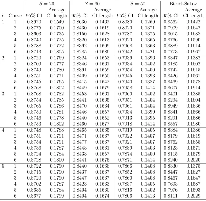
proposed in this paper. For Method (v), we report the cases of S = 20, 30, 50, and
a data-driven method based on Bickel and Sakov (2008) for the subsample size.8 For
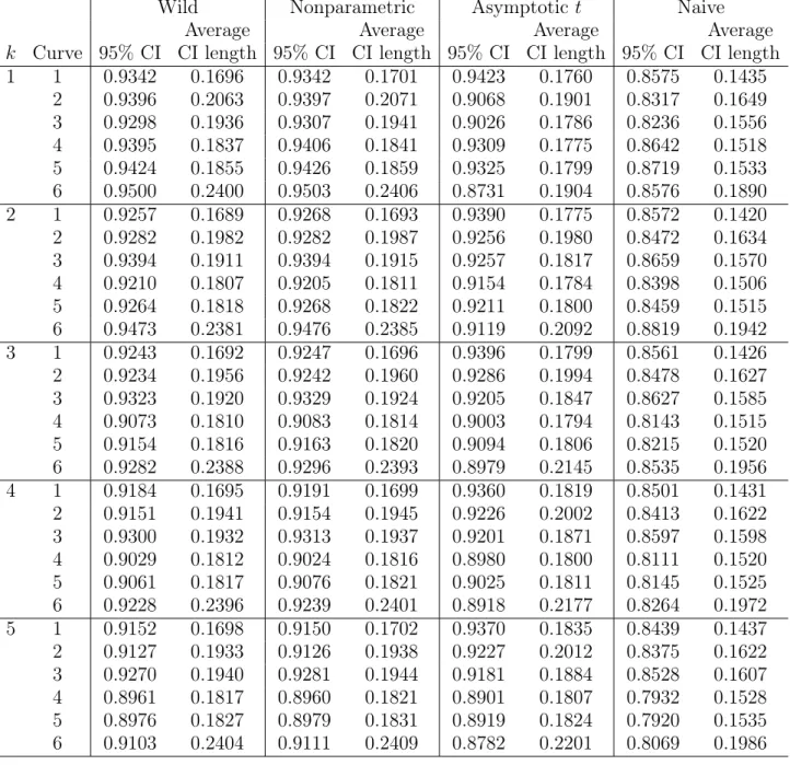
each simulation design, we report coverage rates of the 95% confidence intervals by the above methods. We also report average lengths (over Monte Carlo replications) of the
confidence intervals. The sample size is set as N = 100. Simulation results based on
10,000 replications are presented in Tables 2 and 3.
Our findings are summarized as follows. First, for all cases, the coverage probabilities of the naive bootstrap confidence intervals are below the nominal level. Since the naive
5We tried several different combinations of(γ
1, γ2)and the case wherei follows the centered lognormal with the standard deviation 0.2. Results are similar overall.
6In a preliminary simulation study, results are similar for different values ofM includingM = 1,4, and
16.
7The linear regression is understood to be a special case of the power series estimator ofµ(d, x)presented in Footnote 2. In a preliminary simulation study, we consider different series lengths and find that results are similar overall.
8More precisely, the data-driven subsample size is chosen byS∗= arg min
Sj{supx|LSj(x)−LSj+1(x)|},
whereLSj(·)is the subsampling cumulative distribution function of
p
Sj(˜τSj −˜τ)/σˆSj andSj = 50−2j
bootstrap is asymptotically invalid as shown by Abadie and Imbens (2008), this result
is reasonable.9 Thus, we need to employ other asymptotically valid inference methods.
Second, Tables 3 shows that the coverage rates of the subsampling confidence intervals
are always below the nominal level. The data-driven choice of S does not improve the
under-coverage in general. Furthermore, the results are sensitive to the choice of the
subsample size S. Thus, even though subsampling is asymptotically valid, it does not
work well to approximate the finite sample distribution of the matching estimator in this setup. Third, across all cases, our weighted bootstrap (both wild and nonparametric)
and the asymptotic t confidence intervals by Abadie and Imbens (2006) are reasonably
close to the nominal level. Overall these coverage rates slightly decrease as k = dim(X)
increases, but the results are not sensitive to k. For example, for Curve 1, the coverage
of the wild bootstrap decreases from 0.9342 (for k = 1) to 0.9152 (for k = 5). Fourth,
the average lengths of the weighted bootstrap (wild and nonparametric) are similar to
those of the asymptotict confidence intervals except for some cases where the asymptotic
t shows under-coverage. Finally, for Curve 6, our weighted bootstrap methods (wild and
nonparametric) show better coverage than the asymptotic t method across all cases. For
example, ifk = 1, the coverage of the wild bootstrap confidence interval is 0.9500 but for
the asymptotic t is 0.8731.
Overall our simulation results are encouraging: the weighted bootstrap inference method
developed in this paper is favorably comparable to the asymptotic t method in Abadie
and Imbens (2006, 2011).
We close this section with a remark on the computational cost. For Curve 1 with
k = 1 and N = 100, we implemented 1,000 Monte Carlo replications of the confidence intervals based on the wild and nonparametric bootstrap (with 999 bootstrap replications),
9Abadie and Imbens (2008) showed that the naive bootstrap can produce both under- and over-covarage. In our simulation designs, we only observe under-coverage.
asymptotic t, and subsampling (with S = 20) by a laptop with Intel Core i7-3540M 3.0GHz. In terms of CPU seconds, it takes 11.11 for the wild bootstrap, 11.28 for the
nonparametric bootstrap, 8.85 for the asymptotic t, and 8859.17 for the subsampling.
Also, for N = 8000, one Monte Carlo replication takes 11.16 for the wild bootstrap
(with 29,999 bootstrap repetitions), 7.45 for the nonparametric bootstrap (with 29,999
bootstrap repetitions), 1.70 for the asymptotic t, and 592.70 for the subsampling (with
S = 300). Therefore, except for subsampling, the computational costs to implement these methods are small.
5. Empirical Application
In this section, we apply our weighted bootstrap method to an empirical analysis based on the National Supported Work (NSW) data. The NSW demonstration was a program which aimed to provide subsidized work experience to individuals with longstanding em-ployment problems. The NSW dataset was first analyzed by Lalonde (1986) and subse-quently by Heckman and Hotz (1989), Dehejia and Wahba (1999, 2002) (hereafter, DW), and Smith and Todd (2005) among others. Here we use the dataset uploaded by Rajeev Dehejia (http://users.nber.org/~rdehejia/nswdata2.html). In particular, we analyze two experimental samples and two non-experimental ones. The first experimental sample is also used by Lalonde (1986) (labelled NSW-L). It includes a male sample with ex-addict, ex-offender, and/or high school dropout having complete ex-ante and ex-post earning data. The second experimental sample is also used by DW (labelled NSW-DW). This is a subset of the first experimental sample for males who were randomly assigned in either January to April of 1976 or October of 1976 to August of 1977, and had zero earnings in the 13-24 months before the random assignment. Two non-experimental samples were also analyzed by Lalonde (1986) and DW. The first non-experimental sample is drawn
from the Current Population Survey (labelled CPS) with matched Social Security earn-ings data. It includes all males less than 55 years old. The second non-experimental sample is drawn from the Panel Study Income Dynamics (labelled PSID). It contains all male household heads who were less than 55 years old and did not classify themselves as retired in 1975. We follow the previous studies and focus on the average treatment effect
τt=E[Y
i(1)−Yi(0)|Di = 1] for the treated population. The weighted bootstrap method
for τt and its validity are presented in the web appendix (Section A). From the
experi-mental samples, we can obtain unbiased estimates forτt. We then compute the matching
estimators from the experimental participants and non-experimental control groups from the CPS and PSID.
We first summarize the data. Table 6 reports the means, standard errors (in parenthe-ses), and normalized distances between the experimental and non-experimental samples
of the control groups defined as( ¯X1−X¯0)/
p (S2 0 +S12)/2, whereX¯d= P i:Di=dXi/Ndand Sw = P i:Di=d(Xi− ¯
Xd)2/(Nd−1).10 The two experimental samples (L and
NSW-DW) have similar characteristics except for real earnings in 1975 (RE75). This difference in RE75 is due to the fact that NSW-DW contains more observations with zero earn-ings. On the other hand, the characteristics of the experimental and non-experimental samples (particularly age, marital status, ethnicity, and earnings) are very different. This difference is confirmed by the large normalized distances of the covariates between the experimental treated and non-experimental control groups. Therefore, it is generally dif-ficult to find good matches from these samples.
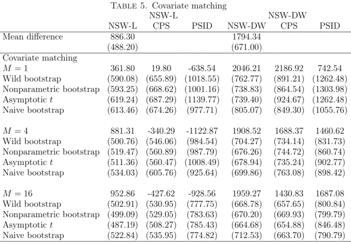
For each pair of samples for the treated and control groups, we implement the matching
estimator for τt and then compute its standard error by Methods (i)-(iv) in Section 4.11
10This normalized distance is employed in Abadie and Imbens (2011). Note that this distance is different from thet-statistic( ¯X1−X¯0)/
p
S2
0/N0+S12/N1to test the null hypothesisE[X1] =E[X0].
11The matching is based on the Mahalanobis distance. The estimator µˆ(d, x) for the bias correction in (2.4) is given by the OLS of the linear regressionµˆi= ˆα+Xiβˆ, which is understood to be a special case
Recall that Methods (i) and (ii) are proposed in this paper, and that Method (iv) (naive
bootstrap) is invalid under fixed-M asymptotics (Abadie and Imbens, 2008). For the
number of matches M, we consider the cases M = 1, 4, and 16.
Table 7 summarizes the results for the matching estimates and standard errors. The first row presents the mean differences between the treatment and control groups. The
unbiased estimates of τt are 886.30 and 1794.34 for the NSW-L and NSW-DW samples,
respectively. The simple covariate matching works well for the NSW-DW sample, but not for the NSW-L sample. For the standard errors, we find that our weighted bootstrap methods (wild and nonparametric) provide similar values as the asymptotic method by Abadie and Imbens (2006). On the other hand, the naive bootstrap standard errors take somewhat different values compared to the others. This result suggests that statistical inference based on the naive bootstrap can be misleading and we recommend employing
asymptotic or weighted bootstrap inference, which are valid under fixed-M asymptotics.
6. Conclusion
This paper proposes a weighted bootstrap inference method for matching estimators of treatment effects. In contrast to the naive bootstrap, our weighted bootstrap method is valid under asymptotics with a fixed number of matches. Our method is applicable to both the average treatment effect and its counterpart for the treated population. Simulation results indicate that the weighted bootstrap method works well in finite samples and is favorably comparable with the asymptotic normal approximation. Although it is beyond the scope of this paper, it would be interesting to investigate higher-order properties of
the weighted bootstrap method under fixed-M asymptotics (see, Kline and Santos, 2012,
for higher-order analysis under standard asymptotics). Also an extension of the weighted
of the power series estimator in Footnote 2. Since results are not sensitive to the length of series, we report only the case of linear regression.
bootstrap method to propensity score matching is currently under investigation by the authors.
Appendix A. Assumptions
Recall µ(d, x) = E[Y|D = d, X = x], σ2(d, x) = V ar(Y|D = d, X = x), and N
0 =
N −N1. Assumptions for the main theorem are listed as follows. All limits are taken as
N → ∞ while M is fixed.
Assumption M. (Conditions for τˆ)
(i): {Yi, Di, Xi}Ni=1 is an i.i.d. sample of (Y, D, X).
(ii): X is continuously distributed on a compact and convex support X ⊂ Rk. The
density of X is bounded and bounded away from zero on X.
(iii): D is independent of (Y(0), Y(1)) conditional on X = x for almost every x. There exists a positive constant c such that Pr{D = 1|X = x} ∈ (c,1−c) for almost every x.
(iv): For eachd∈ {0,1},µ(d, x)andσ2(d, x)are Lipschitz in X, σ2(d, x)is bounded away from zero on X, and E[Y4|D=d, X =x] is bounded uniformly on
X.
Assumption W. (Conditions for W∗)
(i): (W1∗, . . . , WN∗) is exchangeable and independent of Z = (Y,D,X). (ii): PN i=1(W ∗ i −W¯∗)2 p →1, where W¯∗ =N−1PN i=1W ∗ i . (iii): maxi=1,...,N|Wi∗−W¯∗| p →0.
(iv): E[Wi∗2] =O(N−1) for all i= 1, . . . , N.
Let λ= (λ1, . . . , λk)0 be a k-dimensional vector of non-negative integers and∂λa(x) = ∂Pkl=1λla(x)/∂xλ1 1 · · ·∂x λk k . Define |a(·)|m = maxPk l=1λl≤msupx∈X|∂ λa(x)|.
Assumption R. (Conditions for µ(d, x)) For each d ∈ {0,1} and λ satisfying Pk
l=1λl = k, the derivative ∂λµ(d, x) exists and
satisfies supx∈X|∂λµ(d, x)| ≤ C for some C >0. Furthermore, µˆ(d, x) satisfies |µˆ(d,·)− µ(d,·)|k−1 =op(N−1/2+1/k) for each d∈ {0,1}.
Remarks. 1. Assumption M, employed in Abadie and Imbens (2006), is used for
the estimator τˆ. Assumption M (i) is on the sampling process. Assumption M (ii) is
on the distributional form of the covariates X. The assumption that X is continuously
distributed can be relaxed. Discrete covariates with finite support can be accommodated by using subsamples which does not change our main result. On the other hand, for
continuous and high dimensionalX, the assumption that the density ofXis bounded away
from zero can be restrictive. In practice, we can trim observations where the estimated
densities of X are too low. Assumption M (iii) contains standard unconfoundedness and
overlap conditions to identify the average treatment effect τ. Assumption M (iv) lists
boundedness and smoothness conditions for the conditional mean and variance functions. Although Assumption M (iv) is relatively mild, Assumption R typically requires more
stringent conditions on the smoothness of µ(d, x) (particularly for high dimensionalX).
2. Assumption W (i)-(iii) are standard in the literature of the weighted bootstrap (e.g.,
Mason and Newton, 1992). Assumption W (iv) is imposed to deal with the estimation
error of µˆ.
3. Assumption R is imposed to guarantee a sufficiently fast convergence rate on the
bias estimator BˆN in (2.4), i.e.,
√
N( ˆBN − BN) p
→ 0. For example, µˆ(d,·) can be a
series estimator with a suitable choice of series length (see, Footnote 2). Other candidates
of µˆ(d,·) are the kernel estimator and nearest neighborhood estimator with adequate
that varies with N to guarantee fast convergence of the bias estimator. As mentioned
in Footnote 3, when k = dim(X) is large, the last condition typically calls for stringent
smoothness of µ(d, x) inx, such as infinite (or very higher-order) differentiability.
Appendix B. Proof of Theorem
Here we present only the proof of part (i) of the theorem. The proof of part (ii) is
similar. By definition, the bootstrap counterpart T∗ is decomposed as
√ N T∗ = N X i=1 Wi∗(˜τi−τ˜) = N X i=1 (Wi∗−W¯∗)(˜τi−τ˜) = N X i=1 (Wi∗−W¯∗)h(2Di−1){1 +M−1KM(i)}ˆei+ ˆξi i = √N(TN∗ +R∗1N +R∗2N), where √ N TN∗ = N X i=1 (Wi∗−W¯∗)(2Di−1){1 +M−1KM(i)}ei+ξi , √ N R∗1N = N X i=1 (Wi∗−W¯∗)(2Di −1){1 +M−1KM(i)}{µ(Di, Xi)−µˆ(Di, Xi)}, √ N R∗2N = N X i=1 (Wi∗−W¯∗)( ˆξi−ξi).
Thus, it is enough for the conclusion to show that
Pr{√N|R1∗N|> |Z}→p 0, Pr{√N|R2∗N|> |Z}→p 0, (B.1)
for any >0, and
sup r
For (B.1), the definition of R∗1N, (2Di−1)2 = 1, and Assumption W (i) imply E[(√N R∗1N)2|Z] = N E[(W1∗−W¯∗)2]1 N N X i=1 {1 +M−1KM(i)}2{µ(Di, Xi)−µˆ(Di, Xi)}2 +N(N −1)E[(W1∗−W¯∗)(W2∗−W¯∗)] × 1 N(N −1) X i6=j (2Di−1){1 +M−1KM(i)}{µ(Di, Xi)−µˆ(Di, Xi)} ×(2Dj −1){1 +M−1KM(j)}{µ(Dj, Xj)−µˆ(Dj, Xj)} .
Assumption W (iv) guaranteesN E[(W1∗−W¯∗)2] =O(1)andN(N−1)E[(W1∗−W¯∗)(W2∗−
¯
W∗)] = O(1). Therefore, by |µˆ(d,·)−µ(d,·)|k−1 = op(N−1/2+1/k) (Assumption R) and
the fact that E[KM(i)q] is uniformly bounded over N for any q >0 (Lemma 3 of Abadie
and Imbens, 2006), we obtain E[(√N R∗1N)2|Z] →p 0. Then the Markov inequality
im-plies Pr{√N|R∗
1N| > |Z} p
→ 0. A similar argument yields Pr{√N|R∗
2N| > |Z} p → 0. Therefore, we obtain (B.1).
We now show (B.2). Define
ηi = (2Di−1){1 +M−1KM(i)}ei+ξi /√N , so that TN∗ =PN i=1W ∗
i ηi. From Polya’s theorem and Pr
n√
N
σN(˜τ −τ)≤r
o
→Φ(r) for all
r ∈R(Abadie and Imbens, 2006, Theorem 4), it is enough for (B.2) to verify
Pr ( √ N N X i=1 (Wi∗−W¯∗)ηi σN ≤r Z ) −Φ(r)→p 0 for all r ∈R, (B.3)
where Φ(r) is the standard normal distribution function. By Lemma (i) in Appendix C
and PN
i=1(W ∗
i −W¯)2 p
Pr{ZN ≤r|Z} −Φ(r) p →0 for all r∈R, (B.4) where ZN = √ N N X i=1 (Wi∗−W¯∗)ηi q PN i=1(W ∗ i −W¯∗)2 q PN i=1(ηi−η¯)2 , and η¯ = N−1PN
i=1ηi. To show, (B.4), we adapt the argument in Mason and Newton
(1992) to our setup. In particular, let (R1, . . . , RN) be a random vector which takes
each permutation of (1, . . . , N) with equal probability and is independent from Z and
(W1∗, . . . , WN∗). Define ZN∗ =√N N X i=1 (WR∗i−W¯∗)ηi q PN i=1(W ∗ i −W¯∗)2 q PN i=1(ηi−η¯)2 .
Since (W1∗, . . . , WN∗) is exchangeable (Assumption W (i)), ZN and ZN∗ follow the same
distribution. Thus, it is enough for (B.3) to show
Pr{ZN∗ ≤r|Z} −Φ(r)→p 0 for all r∈R,
as N → ∞, or equivalently, every subsequence {Nk}k∈N ⊂ N contains a further
subse-quence {Nk(l)}l∈N ⊂ {Nk}k∈N such that
Pr{ZN∗
k(l) ≤r|Z} −Φ(r) a.s.
→ 0 for all r ∈R, (B.5)
Pick any r∈R. Now define Vi = Wi∗−W¯∗ q PN i=1(W ∗ i −W¯∗)2 , Ui = ηi−η¯ q PN i=1(ηi−η¯)2 , dN(δ) = N X i=1 N X j=1 Ui2Vj2I{N Ui2Vj2 > δ}.
From Assumption W and Lemmas (ii)-(iii), we have
max 1,...,N|Vi| p →0, max 1,...,N|Ui| p →0, dN(δ) p →0, (B.6)
as N → ∞. Pick any subsequence {Nk}k∈N ⊂ N. By (B.6), there exists a further
subsequence {Nk(l)}l∈N ⊂ {Nk}k∈N such that
max 1,...,Nk(l) |Vi| a.s. → 0, max 1,...,Nk(l) |Ui| a.s. → 0, dNk(l)(δ) a.s. → 0, (B.7) as l → ∞. Notice that ZN∗
k(l) is a simple linear rank statistic conditional on Z and
(W1∗, . . . , WN∗
k(l)). Thus, under (B.7), we can apply the rank central limit theorem (Hájek,
1961), that is Pr{ZN∗ k(l) ≤r|Z, W ∗ 1, . . . , W ∗ Nk(l)} −Φ(r) a.s. → 0,
as l→ ∞. Furthermore, the bounded convergence theorem implies
Pr{ZN∗ k(l) ≤r|Z} −Φ(r) = E h Pr{ZN∗ k(l) ≤r|Z, W ∗ 1, . . . , W ∗ Nk(l)} −Φ(r) Z ia.s. → 0,
Appendix C. Lemmas
Lemma. Use the same notation in Appendix B. Under Assumptions M, W, and R in Appendix A, (i) PN i=1(ηi−η¯) 2−σ2 N p →0, (ii)max1,...,N|Ui| p →0, and (iii) dN(δ) p →0, as N → ∞.
Proof of (i). First, we show PN
i=1η 2 i −σN2 p →0. By definition, decompose PN i=1η 2 i = ˆ σ12N + ˆσ22N + 2CN, where ˆ σ12N = 1 N N X i=1 {1 +M−1KM(i)}2e2i, σˆ22N = 1 N N X i=1 (τi−τ)2, CN = 1 N N X i=1 (2Di−1){1 +M−1KM(i)}ei(τi−τ).
The law of large numbers guarantees σˆ22N →p σ22. For σˆ12N, note that
E[(ˆσ21N −σN2)2] = 1 NE {1 +M−1KM(i)}4E[{e2i −σ 2(D i, Xi)}2|Di, Xi] ≤ 1 NE[{1 +M −1K M(i)}4] sup d∈{0,1},x∈X E[e4i|Di =d, Xi =x]→0,
where the convergence follows from Assumption M (iv) and boundedness of E[KM(i)q]
for all q >0uniformly overN (Lemma 3 of Abadie and Imbens, 2006). Thus, the Markov
inequality implies |σˆ2
1N −σ12N| p
→ 0. Similarly, by the Cauchy-Schwarz inequality, we
obtain E[CN2] = 1 NE {1 +M−1KM(i)}2e2i(τi−τ)2 ≤ 1 NE[{1 +M −1K M(i)}4]1/2 E[(τi−τ)4] sup d∈{0,1},x∈X E[e4i|Di =d, Xi =x] !1/2 →0, and thus CN p →0.
Next, we show
¯
η→p 0. (C.1)
Since (a) supd∈{0,1},x∈
XE[|ei||Di = d, Xi = x], (b) supx∈XE[|ξi||Xi =x], and (c) E[{1 +
M−1K
M(i)}] is uniformly bounded overN, we have
E|η| ≤¯ √1
NE[{1 +M
−1K
M(i)}(|ei|+|ξi|)]→0.
Thus, the Markov inequality implies (C.1).
Finally, by using Pn
i=1ηi/σN
d
→N(0,1) (Theorem 4 of Abadie and Imbens, 2006) and
E[σN] =O(1)(Lemma 3 of Abadie and Imbens, 2006), we obtainNη¯=Op(1). Therefore,
combining all these results, we obtain the conclusion as
N X i=1 (ηi −η¯)2−σ2N = N X i=1 ηi2−σ2N ! −Nη¯2 →p 0.
Proof of (ii). By Lemma (i) and (C.1), it is enough to show max1,...,N|ηi| p →0. This follows by Pr max 1,...,N|ηi|> ≤NPr{|ηi|> } ≤ 1 N 4E[({1 +M −1K M(i)}ei +ξi)4]→0,
for any >0, where the first inequality follows from a set inclusion relationship and the
fact that{ηi}Ni=1 are identically distributed, the second inequality follows from the Markov
inequality, and the convergence follows from Assumption M (iv) and uniform boundedness of E[KM(i)q] overN and q >0 (Lemma 3 of Abadie and Imbens, 2006).
Proof of (iii). Pick any >0. It holds that with probability approaching one, dN(δ) ≤ N X i=1 Ui2I{N U2 i > δ/} ≤ δN N X i=1 Ui4 = δ N X i=1 (ηi−η¯)2 !−2 1 N N X i=1 ({1 +M−1KM(i)}ei+ξi)4,
where the first inequality follows from max1,...,N|Vi|
p
→ 0 (by Assumption W (ii)-(iii))
and PN j=1Vj2 = 1. Note that PN i=1(ηi−η¯)2 −2
= Op(1) by Lemma (i) and that σN2 is
uniformly bounded from below (σ2
N ≥infd∈{0,1},x∈Xσ2(d, x)). Thus, if we can show that
1 N N X i=1 ({1 +M−1KM(i)}ei+ξi)4 =Op(1), (C.2)
then we obtain the conclusion by taking arbitrarily small.
It remains to show (C.2). Let γi ={1 +M−1KM(i)}ei+ξi. Note that
γi4 = {1 +M−1KM(i)}4e4i + 4{1 +M −1K M(i)}3e3iξi+ 6{1 +M−1KM(i)}2e2iξ 2 i +4{1 +M−1KM(i)}eiξ3i +ξ 4 i.
By Assumption M (iv), maxq=1,...,4E|ei|q < C for some C > 0. By Abadie and Imbens
(2006, Lemma 3),E[KM(i)q]is uniformly bounded for any q. By the Lipschitz continuity
of µ (Assumption M (iv)) and the compact support of X (Assumption M (ii)), it holds
|ξi|< C0 a.s. for some C0 >0. Combining these results, we can see thatE
h 1 N PN i=1γi4 i
is bounded uniformly over N. Therefore, the Markov inequality implies (C.2), and the
Appendix D. Tables
Table 1. Simulation designs for m(·)
Curves m(z) 1 0.15 + 0.7z 2 0.1 +z/2 + exp(−200(z−0.7)2)/2 3 0.8−2(z−0.9)2−5(z−0.7)3−10(z−0.6)10 4 0.2 +√1−z−0.6(0.9−z)2 5 0.2 +√1−z−0.6(0.9−z)2−0.1zcos(30z) 6 0.4 + 0.25 sin(8z−5) + 0.4 exp(−16(4z−2.5)2) 0.0 0.2 0.4 0.6 0.8 1.0 0.0 0.2 0.4 0.6 0.8 1.0 curve 1 0.0 0.2 0.4 0.6 0.8 1.0 0.0 0.2 0.4 0.6 0.8 1.0 curve 2 0.0 0.2 0.4 0.6 0.8 1.0 0.0 0.2 0.4 0.6 0.8 1.0 curve 3 0.0 0.2 0.4 0.6 0.8 1.0 0.0 0.2 0.4 0.6 0.8 1.0 curve 4 0.0 0.2 0.4 0.6 0.8 1.0 0.0 0.2 0.4 0.6 0.8 1.0 curve 5 0.0 0.2 0.4 0.6 0.8 1.0 0.0 0.2 0.4 0.6 0.8 1.0 curve 6
Table 2. Simulation results for bootstrap and asymptotict methods
Wild Nonparametric Asymptotic t Naive
Average Average Average Average
k Curve 95% CI CI length 95% CI CI length 95% CI CI length 95% CI CI length
1 1 0.9342 0.1696 0.9342 0.1701 0.9423 0.1760 0.8575 0.1435 2 0.9396 0.2063 0.9397 0.2071 0.9068 0.1901 0.8317 0.1649 3 0.9298 0.1936 0.9307 0.1941 0.9026 0.1786 0.8236 0.1556 4 0.9395 0.1837 0.9406 0.1841 0.9309 0.1775 0.8642 0.1518 5 0.9424 0.1855 0.9426 0.1859 0.9325 0.1799 0.8719 0.1533 6 0.9500 0.2400 0.9503 0.2406 0.8731 0.1904 0.8576 0.1890 2 1 0.9257 0.1689 0.9268 0.1693 0.9390 0.1775 0.8572 0.1420 2 0.9282 0.1982 0.9282 0.1987 0.9256 0.1980 0.8472 0.1634 3 0.9394 0.1911 0.9394 0.1915 0.9257 0.1817 0.8659 0.1570 4 0.9210 0.1807 0.9205 0.1811 0.9154 0.1784 0.8398 0.1506 5 0.9264 0.1818 0.9268 0.1822 0.9211 0.1800 0.8459 0.1515 6 0.9473 0.2381 0.9476 0.2385 0.9119 0.2092 0.8819 0.1942 3 1 0.9243 0.1692 0.9247 0.1696 0.9396 0.1799 0.8561 0.1426 2 0.9234 0.1956 0.9242 0.1960 0.9286 0.1994 0.8478 0.1627 3 0.9323 0.1920 0.9329 0.1924 0.9205 0.1847 0.8627 0.1585 4 0.9073 0.1810 0.9083 0.1814 0.9003 0.1794 0.8143 0.1515 5 0.9154 0.1816 0.9163 0.1820 0.9094 0.1806 0.8215 0.1520 6 0.9282 0.2388 0.9296 0.2393 0.8979 0.2145 0.8535 0.1956 4 1 0.9184 0.1695 0.9191 0.1699 0.9360 0.1819 0.8501 0.1431 2 0.9151 0.1941 0.9154 0.1945 0.9226 0.2002 0.8413 0.1622 3 0.9300 0.1932 0.9313 0.1937 0.9201 0.1871 0.8597 0.1598 4 0.9029 0.1812 0.9024 0.1816 0.8980 0.1800 0.8111 0.1520 5 0.9061 0.1817 0.9076 0.1821 0.9025 0.1811 0.8145 0.1525 6 0.9228 0.2396 0.9239 0.2401 0.8918 0.2177 0.8264 0.1972 5 1 0.9152 0.1698 0.9150 0.1702 0.9370 0.1835 0.8439 0.1437 2 0.9127 0.1933 0.9126 0.1938 0.9227 0.2012 0.8375 0.1622 3 0.9270 0.1940 0.9281 0.1944 0.9181 0.1884 0.8528 0.1607 4 0.8961 0.1817 0.8960 0.1821 0.8901 0.1807 0.7932 0.1528 5 0.8976 0.1827 0.8979 0.1831 0.8919 0.1824 0.7920 0.1535 6 0.9103 0.2404 0.9111 0.2409 0.8782 0.2201 0.8069 0.1986
Table 3. Simulation results for subsampling
S = 20 S= 30 S = 50 Bickel-Sakov
Average Average Average Average
k Curve 95% CI CI length 95% CI CI length 95% CI CI length 95% CI CI length
1 1 0.8920 0.1549 0.8630 0.1462 0.8080 0.1269 0.8562 0.1422 2 0.8775 0.1700 0.8430 0.1619 0.8020 0.1371 0.7909 0.1642 3 0.8603 0.1735 0.8150 0.1628 0.7787 0.1375 0.8015 0.1688 4 0.8740 0.1725 0.8320 0.1613 0.7920 0.1365 0.8766 0.1590 5 0.8788 0.1722 0.8392 0.1609 0.7968 0.1363 0.8889 0.1614 6 0.8713 0.1805 0.8285 0.1686 0.7942 0.1421 0.7773 0.1967 2 1 0.8720 0.1769 0.8324 0.1653 0.7939 0.1396 0.8347 0.1382 2 0.8709 0.1777 0.8346 0.1661 0.7934 0.1402 0.8185 0.1602 3 0.8749 0.1780 0.8391 0.1659 0.7954 0.1400 0.8742 0.1615 4 0.8751 0.1771 0.8409 0.1650 0.7945 0.1393 0.8426 0.1561 5 0.8745 0.1765 0.8415 0.1642 0.7940 0.1387 0.8469 0.1578 6 0.8768 0.1802 0.8449 0.1679 0.7958 0.1414 0.8607 0.1914 3 1 0.8768 0.1782 0.8453 0.1661 0.7960 0.1402 0.8401 0.1385 2 0.8754 0.1785 0.8441 0.1665 0.7951 0.1404 0.8294 0.1604 3 0.8765 0.1786 0.8470 0.1664 0.7961 0.1404 0.8949 0.1636 4 0.8750 0.1781 0.8446 0.1657 0.7934 0.1399 0.8341 0.1566 5 0.8746 0.1778 0.8440 0.1652 0.7913 0.1395 0.8291 0.1586 6 0.8753 0.1802 0.8460 0.1677 0.7918 0.1414 0.8557 0.1980 4 1 0.8748 0.1788 0.8465 0.1665 0.7919 0.1405 0.8384 0.1386 2 0.8751 0.1791 0.8471 0.1667 0.7922 0.1407 0.8179 0.1619 3 0.8754 0.1791 0.8477 0.1667 0.7921 0.1407 0.8762 0.1655 4 0.8736 0.1787 0.8448 0.1661 0.7889 0.1403 0.8123 0.1571 5 0.8724 0.1784 0.8433 0.1657 0.7874 0.1400 0.8115 0.1579 6 0.8728 0.1800 0.8441 0.1675 0.7871 0.1414 0.8240 0.2020 5 1 0.8722 0.1790 0.8440 0.1666 0.7866 0.1408 0.8330 0.1375 2 0.8715 0.1790 0.8437 0.1667 0.7852 0.1408 0.8447 0.1627 3 0.8720 0.1790 0.8447 0.1667 0.7860 0.1408 0.8467 0.1647 4 0.8702 0.1787 0.8423 0.1663 0.7837 0.1405 0.7693 0.1587 5 0.8685 0.1784 0.8404 0.1660 0.7816 0.1402 0.7976 0.1593 6 0.8677 0.1799 0.8404 0.1674 0.7806 0.1413 0.8111 0.2029
Table 4. Summary statistics
# of obs Age Education Black Hispanic
NSW-L Treated 297 24.63 10.38 .80 .09 (6.69) (1.82) (.40) (.29) Control 425 24.45 10.19 .84 .11 (6.59) (1.62) (.40) (.32) NSW-DW Treated 185 24.45 10.19 .84 .06 (7.16) (2.01) (.36) (.24) Control 260 25.05 10.09 .83 .11 (7.06) (1.61) (.38) (.31) PSID 2,490 34.85 12.11 .25 .03 (10.44) (3.08) (.43) (.18) CPS 15,992 33.22 12.02 .07 .07 (11.05) (2.87) (.26) (.25 ) Normalized difference NSW-L T/C .03 .11 .003 -.06 NSW-L/PSID -1.17 -.69 1.32 -1.95 NSW-L/CPS -0.94 -.69 2.16 -1.31 NSW-DW T/C .11 .14 .04 -.17 NSW-DW/PSID -1.01 -.68 1.48 .13 NSW-DW/CPS -.80 -.68 2.43 -.05
No degree Married RE74 RE75
NSW-L Treated .73 .17 3,066 (.37) (.44) (4,874) Control .81 .16 3,026 (.36) (.39) (5,201) NSW-DW Treated .71 .19 2,095 1,532 (.39) (.46) (4,886) (3,219) Control .83 .15 2,107 1,267 (.36) (.37) (5,687) (3,102) PSID .31 .87 19,429 19,063 (.46) (.34) (13,406) (13,596) CPS .29 .71 14,016 13,650 (.45) (.46) (9,570) (9,270) Normalized difference NSW-L T/C -.20 .03 .008 NSW-L/PSID .26 .94 -1.57 NSW-L/CPS .08 .97 -1.43 NSW-DW T/C -.30 .09 -.002 .08 NSW-DW/PSID .88 -1.84 -1.72 -1.77 NSW-DW/CPS .90 -1.23 -1.57 -1.75
Table 5. Covariate matching NSW-L NSW-DW NSW-L CPS PSID NSW-DW CPS PSID Mean difference 886.30 1794.34 (488.20) (671.00) Covariate matching M = 1 361.80 19.80 -638.54 2046.21 2186.92 742.54 Wild bootstrap (590.08) (655.89) (1018.55) (762.77) (891.21) (1262.48) Nonparametric bootstrap (593.25) (668.62) (1001.16) (738.83) (864.54) (1303.98) Asymptotict (619.24) (687.29) (1139.77) (739.40) (924.67) (1262.48) Naive bootstrap (613.46) (674.26) (977.71) (805.07) (849.30) (1055.76) M = 4 881.31 -340.29 -1122.87 1908.52 1688.37 1460.62 Wild bootstrap (500.76) (546.06) (984.54) (704.27) (734.14) (831.73) Nonparametric bootstrap (519.47) (560.89) (987.79) (676.26) (744.72) (860.74) Asymptotict (511.36) (560.47) (1008.49) (678.94) (735.24) (902.77) Naive bootstrap (534.03) (605.76) (925.64) (699.86) (763.08) (898.42) M = 16 952.86 -427.62 -928.56 1959.27 1430.83 1687.08 Wild bootstrap (502.91) (530.95) (777.75) (668.78) (657.65) (800.84) Nonparametric bootstrap (499.09) (529.05) (783.63) (670.20) (669.93) (799.79) Asymptotict (487.19) (508.27) (785.43) (664.68) (654.88) (846.48) Naive bootstrap (522.84) (535.95) (774.82) (712.53) (663.70) (790.79) References
[1] Abadie, A. and G. W. Imbens (2006) Large sample properties of matching estimators for average treatment effects,Econometrica, 74, 235-267.
[2] Abadie, A. and G. W. Imbens (2008) On the failure of the bootstrap for matching estimators,
Econometrica, 76, 1537-1557.
[3] Abadie, A. and G. W. Imbens (2011) Bias-corrected matching estimators for average treatment effects,Journal of Business & Economic Statistics, 29, 1-11.
[4] Abadie, A. and G. W. Imbens (2012) A Martingale representation for matching estimators,Journal of the American Statistical Association, 107, 833-843.
[5] Bickel, P. J. and A. Sakov (2008) On the choice ofm in them out of n bootstrap and confidence bounds for extrema,Statistica Sinica, 18, 967-985.
[6] Busso, M., DiNardo, J. and J. McCrary (2014) New evidence on the finite sample properties of propensity score matching and reweighting estimators,Review of Economics and Statistics, 96, 885-897.
[7] Cattaneo, M. D., Crump, R. K. and M. Jansson (2010) Robust data-driven inference for density-weighted average derivatives,Journal of the American Statistical Association, 105, 1070-1083. [8] Cattaneo, M. D., Crump, R. K. and M. Jansson (2014) Bootstrapping density-weighted average
derivatives,Econometric Theory, 30, 1135-1164.
[9] Dehejia, R. and S. Wahba (1999) Causal effects in nonexperimental studies: reevaluating the evalu-ation of training programs,Journal of the American Statistical Association, 94, 1053-1062.
[10] Dehejia, R. and S. Wahba (2002) Propensity score-matching method for nonexperimental causal studies,Review of Economics and Statistics, 84, 151-161.
[11] Efron, B. (1979) Bootstrap methods: Another look at the jackknife, Annals of Statistics, 7, 1-26. [12] Frölich, M. (2004) Finite-sample properties of propensity-score matching and weighting estimators,
Review of Economics and Statistics, 86, 77-90.
[13] Hájek, J. (1961) Some extensions of the Wald-Wolfowitz-Noether theorem,Annals of Mathematical Statistics, 32, 506-523.
[14] Heckman, J. and J. Hotz (1989) Choosing among alternative nonexperimental methods for estimating the impact of social programs: the case of manpower training,Journal of the American Statistical Association, 84, 862-874.
[15] Heckman, J., Ichimura, H. and P. Todd (1998) Matching as an econometric evaluation estimator,
Review of Economic Studies, 65, 261-294.
[16] Hirano, K., Imbens, G. and G. Ridder (2003) Efficient estimation of average treatment effects using the estimated propensity score,Econometrica, 71, 1161-1189.
[17] Kline, P. and A. Santos (2012) Higher order properties of the wild bootstrap under misspecification,
Journal of Econometrics, 171, 54-70.
[18] Lalonde, R. J. (1986) Evaluation the econometric evaluations of training programs with experimental data,American Economic Review, 76, 604-620.
[19] Mammen, E. (1993) Bootstrap and wild bootstrap for high dimensional linear models, Annals of Statistics, 21, 255-285.
[20] Mason, D. M. and M. A. Newton (1992) A rank statistics approach to the consistency of a general bootstrap,Annals of Statistics, 20, 1611-1624.
[21] Pauly, M. (2011) Weighted resampling of martingale difference arrays with applications, Electronic Journal of Statistics, 5, 41-52.
[22] Politis, N. and J. Romano (1994) Large sample confidence regions based on subsamples under min-imal assumptions,Annals of Statistics, 22, 2031-2050.
[23] Rubin, D. (1981) The Bayesian bootstrap,Annals of Statistics, 9, 130-134.
[24] Smith, J. and P. Todd (2005) Does matching address Lalonde’s critique of nonexperimental estima-tors?,Journal of Econometrics, 125, 305-353.
[25] Stone, C. J. (1977) Consistent nonparametric regression,Annals of Statistics, 5, 595-620.
[26] Wu, C. F. J. (1986) Jackknife, bootstrap, and other resampling methods in regression analysis,
Annals of Statistics, 14, 1261-1295.
Department of Economics, London School of Economics, Houghton Street, London, WC2A 2AE, UK.
E-mail address: [email protected]
Department of Economics, University of Wisconsin-Madison, 1180 Observatory Drive, Madison, WI 53706, USA.