for discretely observed compound
Poisson processes
Alberto Jes´
us Coca Cabrero
Darwin College
University of Cambridge
A thesis submitted for the degree of
Doctor of Philosophy
Compound Poisson processes are the textbook example of pure jump stochastic processes and the building blocks of L´evy processes. They have three defining parameters: the distribution of the jumps, the intensity driving the frequency at which these occur, and the drift. They are used in numerous applications and, hence, statistical inference on them is of great interest. In particular, nonparametric estimation is increasingly popular for its generality and reduction of misspecification issues.
In many applications, the underlying process is not observed directly but at discrete times. Therefore, important information is missed between observations and we face a (non-linear) inverse problem. Using the intimate relationship between L´evy processes and infinite divisible distributions, we construct new estimators of the jump distribution and of the so-called L´evy distribution. Under mild assumptions, we prove Donsker theorems for both (i.e. functional central limit theorems with the uniform norm) and identify the limiting Gaussian processes. This allows us to conclude that our estimators are efficient, or optimal from an information theory point of view, and to give new insight into the topic of efficiency in this and related problems. We allow the jump distribution to potentially have a discrete component and include a novel way of estimating the mass function using a kernel estimator. We also construct new estimators of the intensity and of the drift, and show joint asymptotic normality of all the estimators. Many relevant inference procedures are derived, including confidence regions, goodness-of-fit tests, two-sample tests and tests for the presence of discrete and absolutely continuous jump components.
In related literature, two apparently different approaches have been taken: a natural direct approach, and the spectral approach we use. We show that these are formally equiv-alent and that the existing estimators are very close relatives of each other. However, those from the first approach can only be used in small compact intervals in the positive real line whilst ours work on the whole real line and, furthermore, are the first to be efficient. We describe how the former can attain efficiency and propose several open problems not yet identified in the field. We also include an exhaustive simulation study of our and other estimators in which we illustrate their behaviour in a number of realistic situations and their suitability for each of them. This type of study cannot be found in existing literature and provides several insights not yet pointed out and solid understanding of the practical side of the problem on which real-data studies can be based. The implementation of all the estimators is discussed in detail and practical recommendations are given.
I am all too aware that the completion of my doctoral studies would not have been possible were it not for the generous support of so many. Herein, I express my deep gratitude to all who have contributed to making this journey a unique, meaningful and life-changing experience.
Firstly, I wish to thank my doctoral supervisors —Richard Nickl and L. Christopher G. Rogers. To Richard, my principal supervisor, because he not only introduced me to the fascinating world of nonparametric statistics but his passion for the subject has enthused me and his mentoring has opened up the academic world; I am only so honoured I will continue having the opportunity to learn from his immense mathematical knowledge after the Ph.D in a Post Doc with him. I wish too to thank Chris for sharing his exceptional insights into some challenging probability open problems, as well as for his dedication and personal support.
I would like to express my gratitude to the CCA and its directors for putting their trust in me when they accepted me onto what has been a fantastic Ph.D. programme and to the CCA administrators for their continued support; I am especially thankful to CCA director James Norris for acting as internal examiner in my defence. I am similarly grateful to Markus Reiß for acting as external examiner; the defence was a truly enriching experience in which a number of exciting future lines of research arose. I am also very much indebted to Markus for his hospitality during two visits to Berlin. I consider myself most fortunate for the rest of the people who have walked this journey with me and who have provided me with a firm personal support of incalculable value. My utmost gratitude must go to my family; especially to my parents, siblings, and grandmothers. They have loved me unconditionally throughout by being the pillar on which I could always rely to rest on and by showing boundless generosity. Most especially, to my parents, Jes´us Coca Grad´ın and Purificaci´on Cabrero Maroto, who have taught me the most important lessons in life and without which I would not have been able to succeed in this enterprise. A few lines herein would never suffice to thank you enough: every achievement of mine is yours.
I am most grateful to my beloved friends; unfortunately, I do not have enough space to thank them all. To Alexandra Gandini who, after my family, has been my greatest influence, both personally and professionally; I wish you and your family the very best. To my childhood friends, Jorge D´avila, Javier Gonz´alez-Adalid, Clara L´opez and Robert
Mathew Edwards, Douwe Kiela and Kattria van der Ploeg, who have made these years be truly outstanding, not only through memorable experiences but also through the highly stimulating academic discussions I was fortunate to have with them. To Simon Walsh, an exceptional friend and an inspirational man who keeps challenging me intellectually and who was always there in tough times. To the mathematicians, Milana Gatari´c, Gil Ramos and Martin Taylor, for their sincere friendships, for the exciting mathematical discussions we have had and for the invaluable advice they have provided me with to navigate through the academic world. And to Julia L´opez Canelada, for her immeasurable patience and generous support whilst writing this thesis, a truly
demanding period that she illuminated with her everlasting happiness and radiant smile. Thank you all for giving me the opportunity to share the joy of life and knowledge with you and I can only hope to be honoured to continue doing so in the near future.
I wish also to recognise the generosity and support I received from many organisations during the course of my Ph.D. studies: Fundaci´on “La Caixa”, EPSRC, Fundaci´on Mutua Madrile˜na, Access to Learning Fund, Cambridge Philosophical Society, Lundgren Fund and Darwin College.
And lastly, to luck, for all the above and much more: please, receive my most profound gratitude.
This dissertation is the result of my own work and includes nothing which is the outcome of work done in collaboration. It is not substantially the same as any that I have submit-ted, or, is being concurrently submitted for a degree or diploma or other qualification at the University of Cambridge or any other University or similar institution. I further state that no substantial part of my dissertation has already been submitted, or, is being con-currently submitted for any such degree, diploma or other qualification at the University of Cambridge or any other University of similar institution.
Abstract iii Acknowledgements vii Declaration ix Contents xiii List of Notation 1 1 Introduction 3
1.1 Compound Poisson processes . . . 3
1.2 Why nonparametric estimation? . . . 7
1.3 Estimation of compound Poisson processes from continuous observations . 8 1.3.1 The estimation problem . . . 8
1.3.2 A glimpse of empirical process theory and of asymptotic efficiency 9 1.4 Estimation of compound Poisson processes from discrete observations . . 12
1.4.1 The estimation problem . . . 12
1.4.2 A brief history of the solution to the problem . . . 14
1.5 Organisation and contributions of the thesis . . . 17
1.5.1 Chapter 2 . . . 17
1.5.2 Chapter 3 . . . 17
1.5.3 Chapter 4 . . . 18
2 Unifying existing literature 19 2.1 The direct approach . . . 19
2.1.1 Compound distributions . . . 20
2.1.2 Nonparametric estimation with the direct approach . . . 20
2.2 The spectral approach . . . 27
2.2.1 L´evy processes . . . 28
2.2.2 Nonparametric estimation with the spectral approach . . . 29
2.3.1 The formal equivalence . . . 39
2.3.2 Similarities between existing estimators . . . 41
2.4 Estimators of the intensity and the drift . . . 43
2.4.1 Estimating the intensity . . . 43
2.4.2 Estimating the drift . . . 47
2.5 Estimators of the process . . . 50
2.6 Asymptotic efficiency of the estimators . . . 53
3 Theory 61 3.1 Definitions and notation . . . 61
3.2 Assumptions and estimators . . . 62
3.3 Central limit theorems . . . 67
3.4 Proofs . . . 72
3.4.1 Joint convergence of one-dimensional distributions . . . 72
3.4.2 Proof of Propositions 3.3.1 and 3.3.3 . . . 92
3.4.3 Proof of Theorem 3.3.4 . . . 92 3.4.3.1 Estimation of N . . . 92 3.4.3.2 Estimation of F . . . 98 3.4.4 Proof of Theorem 3.3.5 . . . 102 3.4.5 Proof of Lemma 3.3.2 . . . 105 4 Applications 107 4.1 Introduction . . . 107
4.2 Statistical procedures and their construction . . . 108
4.2.1 Approximating the limiting processes . . . 109
4.2.2 Confidence regions . . . 112
4.2.3 Goodness-of-fit tests . . . 113
4.2.4 Two-sample tests . . . 114
4.2.5 Approximations for λ∆ sufficiently small . . . 115
4.3 Implementation . . . 117
4.3.1 Spectral approach-based estimators . . . 117
4.3.2 Direct approach-based estimators . . . 123
4.4 Simulated illustrations . . . 126
4.4.1 Preliminary remarks . . . 127
4.4.1.1 Division of Section 4.4 . . . 127
4.4.1.2 Remarks on the practical implementation . . . 129
4.4.1.3 A guide to read the tables . . . 131
4.4.2 Moderate intensity (1≤λ.5) . . . 132
4.4.3 High intensity (λ&5) . . . 137
4.4.5 Conclusions and remarks . . . 142 4.4.6 Further investigations . . . 144
∆ The size of the time-increments at which a stochastic process is (discretely) observed
F,F(·) The distribution function of the underlying jumps of a compound Poisson process
e
F ,Fe(·),F ,b Fb(·) Estimators ofF of Buchmann and Gr¨ubel [2003] and Coca [2015],
respectively
F,F−1 The Fourier(–Plancherel) transform and its inverse transform
γ The drift of a compound Poisson process
˜
γ,γˆ Estimators of γ (naive and spectral of Coca [2015], respectively) h,hn The bandwidth of a kernel function
n Size of a sample
i.i.d. Independent and identically distributed
K A kernel function
λ The intensity of a compound Poisson process
˜
λ,λ,ˆ λˇ Estimators of λ(naive, spectral mass of Coca [2015] and spectral origin, respectively)
`∞(C) Space of real-valued uniformly bounded functions on C⊆R L∞(C) Equivalence class of real-valued essentially bounded functions on
C ⊆R
Lr(C),1≤r <∞ Equivalence class of real-valued, Lebesgue-measurable functions f on C⊆Runder the normkfkr := R
C|f(x)| rdx1/r
Log, log The distinguished and the natural logarithms
L,L−1 The Laplace transform and its inverse transform
max,∨ Maximum
min,∧ Minimum
µ A finite measure
(Nt)t≥0 A Poisson process
N, N(·) The L´evy distribution function
b
N ,Nb(·) Estimator of N of Coca [2015]
NG, NG(·) The generalised L´evy distribution function
b
NG,NbG(·) Estimator of NG of Nickl and Reiß [2012]
N,N(·) A functional of the L´evy measure
b
N,Nb(·) Estimator of N of Nickl et al. [2016]
N The set of natural numbers (nonnegative integer numbers)
ν The L´evy measure
O, o Big-O and small-o notation
OP r Big-O notation in P r-probability (Ω,A, P r) The underlying probability space
P,Pn The law of an increment of a L´evy process and its empirical coun-terpart
ϕ,ϕn The characteristic function of a L´evy process and its empirical coun-terpart
Re, Im The real and the imaginary parts of complex number
R The set of real numbers
Rd The d-dimensional Euclidean space
supp(·) The support of a function
T The total length of the observation interval
(Xt)t≥0 A L´evy process (generally compound Poisson process) Y1, Y2, . . . The underlying jumps of a compound Poisson process Z1, . . . , Zn The increments of a discretely observed L´evy process
Z The set of integer numbers
bxc The greatest integer less or equal tox k · k`∞(C) Uniform or supremum norm on C⊆R k · k∞ Short version of k · k`∞(
R)
k · k∞,τ The (τ-)exponentially downweighted uniform norm on R+,
supx≥0|e−τ xf(x)|withτ ≥0 k · kT V Total variation norm
→d Classical convergence in distribution
→D Convergence in distribution in the sense introduced by Hoffmann-Jørgensen
.,& Uniform order relations
Introduction
The purpose of this chapter is to introduce the problem we solve in this thesis: to make efficient nonparametric inference on discretely observed compound Poisson processes. In Section 1.1 we introduce these processes and some of their probabilistic properties, which are exploited in subsequent chapters. Based on this, in Section 1.2 we justify why when making statistical inference on them we take a nonparametric approach instead of a more classical parametric one. In Sections 1.3 and 1.4 we introduce nonparametric estimation of compound Poisson processes in two different frameworks depending on the type of data available to the statistician: in the first, the process is fully observed, whilst in the second it is only observed at discrete times. Estimation in the first framework follows from standard results in mathematical statistics. Nonetheless, it allows us to naturally motivate the type of results that are the focus of this thesis and which are developed in the second framework. In Section 1.4 we state the exact problem that concerns us here, and in Section 1.5 we clearly indicate our contributions to it and give an outline of the rest of the thesis.
1.1
Compound Poisson processes
Compound Poisson processes are one of the most basic examples of continuous-time pure-jump stochastic processes. Nevertheless, they provide enough flexibility to model a large number of phenomena observed in numerous fields. They are highly tractable from a mathematical point of view and are building blocks of many more elaborated stochastic processes such as queues and L´evy processes.
The construction of a compound Poisson process can be summarised as follows: (a) the occurrence of the jumps is determined by a Poisson process;
(c) the interarrival times between jumps and the size of the jumps are mutually inde-pendent random variables; and,
(d) the process may increase or decrease steadily due to a drift factor.
In mathematical terms, let (Nt)t≥0 be a d-dimensional Poisson process with intensity λ > 0. Let Y1, Y2, . . . be a sequence of independent and identically distributed (i.i.d.) random variables taking values inRdwith common distributionF. Assume this sequence
is independent of the Poisson process and let γ ∈ Rd. Then a d-dimensional compound Poisson process (Xt)t≥0 with drift γ, intensity λ and jump size distribution F can be written as Xt=γt+ Nt X j=1 Yj, t≥0, (1.1.1)
where an empty sum is zero by convention so, in particular, the process always starts at zero. Figure 1.1 illustrates a typical path of a one-dimensional compound Poisson process without drift. In what follows we concentrate on the cased= 1.
Figure 1.1: (Xt)t∈[0,10] withγ= 0,λ= 0.5 andF =N(0,1)
A one-dimensional Poisson process with intensityλcan be constructed as follows. Let E1, E2, . . . be a sequence of independent and identically distributed exponential random variables with parameterλ, with the convention that λ−1 is their expected value. Then the Poisson process can be written as
Nt= max k∈N: k X j=1 Ej ≤t , t≥0,
where, again, an empty sum is zero by convention so, in particular, the process always starts at zero. From this construction it is apparent that the interarrival times of the compound Poisson process are exponentially distributed. As pointed out in Section 5.4 in Bingham and Kiesel [2004], the exponential distribution is special in that, subject
to minimal regularity assumptions, it is the only distribution with the so-called lack-of-memory property: if (Ω,A, P r) denotes the underlying probability space on which all random elements of this thesis are defined, then
P r(E1 > s+t|E1 > s) =P r(E1 > t), for all s, t >0. (1.1.2) This property provides the compound Poisson process with the (strong) Markov property, which makes it very mathematically tractable. In particular, it means that the survival function of the interarrival distributions does not change depending on where we observe them. Intuitively, the random time of occurrence of a jump shows no ageing. Consequently, compound Poisson process are used in numerous applications to model random events that occur ‘out of the blue’.
In order to gain more intuition into these processes, let us introduce two applications in which they are used. These also motivate the division between Section 1.3 and Section 1.4. Consider an ATM where deposits can be made. Customers arrive at random and withdraw or deposit a random amount of money. The interest of an ATM manager is to understand how much money is likely to be enough to cover the random transactions without having to risk introducing too much of it in the machine. In normal conditions, the assumptions of mutually independent exponential interarrival times andF-distributed amounts of money are satisfied. However, the homogeneity in the underlying parameters may be violated, so in practice the model is applied after splitting the observations into time-intervals where this is a reasonable assumption. A second example comes from ecology. Consider a nature reserve where groups of birds stop in the course of their migration. Within certain weeks of the year they arrive and leave at random with an approximately constant intensity rate. Furthermore, and in those weeks, the size of their groups also varies randomly according to an approximately homogeneous-in-time distribution. A manager of the park requires to understand the minimum and maximum number of birds that typically occupy a certain area to build appropriate infrastructure. Therefore, in both applications the one observes the aggregated effect of all the random events and this justifies the practical importance of compound Poisson processes. As we mention in Sections 1.3 and 1.4, the difference between the two is the frequency at which the process is observed. In either case, the challenge is to estimate the defining parameters of the underlying process, all of which are generally unknown to the practitioner. Although we discuss estimation of all, the most challenging one isF and this is the focus of this thesis.
Returning to the mathematical properties of the compound Poisson process, the lack-of-memory property and the independence assumptions imply it belongs to the wider class of L´evy processes. In other words, (Xt)t≥0as defined above enjoys the following properties (cf. Sato [1999]):
zero; and,
(ii) it has stationary and independent increments.
The second is the key property of L´evy processes. It has been extensively exploited to make statistical inference on them and so do we in subsequent chapters. Furthermore, it gives rise to the intimate relationship that these processes have with infinitely divisible distributions, which were introduced by De Finetti [1929]. As a consequence, and as shown by L´evy [1934], Khintchine [1937] and Itˆo [1942], the characteristic function of a L´evy process at a certain time is given by the L´evy-Khintchine formula, which explicitly depends on the defining parameters of the process. This can be exploited to build estimators of them, especially when having discrete observations of the process. Indeed, it is the starting point of the so-called spectral approach, which we introduce in Section 2.2 and use in Chapter 3 to show our novel results. We postpone introducing the formula in full generality until Section 2.2.1 and for now we focus on its expression for the case of a compound Poisson process. For this purpose, let E denote the expectation under P r and let F denote the
Fourier (–Plancherel) transform acting on finite measures with the convention
Fµ(u) =
Z
R
eiuxµ(dx), u∈R. (1.1.3)
Then, by a simple calculation using (1.1.1), the characteristic function ofXtcan be written as
ϕt(u) :=E[eiuXt] =et iuγ+Fν(u)−λ
, t≥0, u∈R, (1.1.4) whereν is generally referred to as the L´evy measure and it satisfiesν =λ dF. Throughout we denote the measure associated to a distribution functionF bydF. Note, in particular, that
−2λ≤Re(Fν(u)−λ)≤0 and |Im(Fν(u)−λ)| ≤λ, u∈R, (1.1.5)
and therefore
1≥ inf
u∈R|ϕt(u)| ≥e
−2λt>0, t >0. (1.1.6) We repeatedly use these properties in subsequent sections and chapters. We remark that from now on we assumeF has no atom at the origin. This is a harmless requirement that guarantees identifiability all of the parameters: otherwise, if a jump can take the value zero, the process does not jump and the mass of such atom cannot be identified. For the same reason, estimation of the intensity cannot be performed. Indeed, ifp0 ∈[0,1) is the mass ofdF at the origin, identity (1.1.4) can be written as
ϕt(u) :=et iuγ+Fν0(u)−λ0
whereν0:=λ0dF0,λ0 :=λ(1−p0) anddF0 := (1−p0)−1(dF−p0δ0). Therefore, the zero jumps coming fromp0 and the flat areas arising fromλtangle up to be indistinguishable from a process with intensity λ0, and this is the only parameter that can be identified. Moreover, all the compound Poisson processes resulting from all possible choices ofp0 ∈
[0,1) and λ > 0 for which the product λ(1−p0) remains constant are indistinguishable from each other. Consequently, we may assumep0= 0 without loss of generality and this way avoid the lack of identifiability of the parameters p0 and λ.
The statistical relevance of identity (1.1.4) is the following: assume we only have i.i.d. observations ofXt for some t≥0 fixed. Then, due to the definition of ϕt as an expecta-tion, it is possible to approximate it by its empirical version, the empirical characteristic function. The idea of the spectral approach to construct estimators is to find relationships between each of the parameters and the characteristic function using (1.1.4), and to ‘plug in’ the empirical version of the latter in place of it. As it should be clear by now, the fact thatϕt is the Fourier transform of the law of Xt, and that we are hence resorting to the frequency domain to construct estimators, gives the whole approach the name of spectral approach. We postpone giving more details of it until the next chapter.
1.2
Why nonparametric estimation?
The most classical branch of statistics is concerned with making conclusions on models that are defined through a finite-dimensional parameter. This is coined parametric statistics and has a long history dating back to J. Bernoulli, A. de Moivre and T. Bayes in the 18th century and further developed by P. S. Laplace and C. F. Gauss in the late 18th and early 19th centuries. Its mathematical foundations were laid in the first half of the 20th century by the remarkably mathematically-gifted biologist R. A. Fisher and, in the second half of the century, the mathematical theory was finally formalised and unified to its modern form by L. M. Le Cam. For an extensive account on its fascinating history we refer the reader to Hald [2007], and for a comprehensive account of its mathematical foundations to van der Vaart [1998]. One of the advantages of parametric procedures is that generally they are simple to formulate and fast to compute. However, in many modern practical situations there is no reason to believe the assumption of the data being generated by a specific finite-dimensional model is correct. In fact, this assumption naturally gives rise to the problem of robustness to the choice of model.
Recall that in the definition of the compound Poisson process above no assumptions were made on the distributionF other than it having no mass at the origin. Consequently, the main estimation problem that concerns us here is that of estimating a family of functionals of a general probability measure and it naturally falls into the realm of inference on infinite-dimensional models or nonparametric statistics. The development of this branch is more contemporary than that of parametric statistics and arguably began in the 1930s
with Glivenko–Cantelli’s theorem, independently proved by Glivenko [1933] and Cantelli [1933], and the Kolmogorov–Smirnov statistic studied in Kolmogorov [1933] and Smirnov [1939]. We note in passing that this coincides with the development of the study of L´evy processes mentioned above. As a result of the advent of powerful computers and the new and challenging modelling demands, the last few decades have witnessed the largest development of this field and it currently is a very active area of research. We refer the reader to the recent and unified account of its mathematical foundations given in Gin´e and Nickl [2016]. In contrast to parametric statistical procedures, nonparametric analogues do not suffer as much from the highly undesirable drawback of model misspecification. For all these reasons herein we focus on nonparametric estimation of compound Poisson processes.
A thoughtful reader may argue that we are making a parametric assumption by letting the interarrival times be exponentially distributed. Nonetheless, we emphasise that we are interested in modelling a process with jumps whose occurrence shows no ageing, because in many applications this is a reasonable approximation. This qualitative property, depicted by (1.1.2), is mathematically equivalent to requiring that the survival function of the interarrival distribution satisfies the Cauchy-functional equation f(x +y) = f(x)f(y), x, y∈R. As mentioned above, the only solution to this functional equation under minimal
regularity assumptions is the parametric exponential distribution. The drift term can also be generalised to a time-dependent function but, in the discrete observation setting introduced in Section 1.4 and considered in the rest of the chapters, strong assumptions have to be made to obtain weak conclusions. We therefore lose almost no generality by assuming the relevant-in-practice modelling assumption of a linear deterministic function in (1.1.1).
1.3
Estimation of compound Poisson processes from
con-tinuous observations
We begin introducing the problem of nonparametric estimation of compound Poisson pro-cess under a simple observation assumption. We do this in Section 1.3.1, where we also give its solution. Then, in Section 1.3.2 we briefly discuss a few concepts from empiri-cal process theory and information theory arising from it. These are repeatedly used in subsequent chapters and the section serves as a natural motivation for the results therein.
1.3.1 The estimation problem
Recall the example of the ATM introduced in Section 1.1. At the end of the day, the ATM manager can access the machine’s database and see the time at which each transaction took place and its value, just as in Figure 1.1. Therefore, there exists aT >0 such that they
observe Xt for all t∈ [0, T]. This is commonly referred to as the continuous observation scheme. In this case,γ is observed directly and so are the independent interarrival times E1, . . . , ENT and the independent jumpsY1, . . . , YNT. Thus, classical statistical techniques can be used to estimate λand F (cf. van der Vaart [1998]): if we condition onNT =m, the intensity can be estimated by the maximum likelihood estimator
λm:= 1 1 m Pm j=1Ej
and the jump distribution function by the empirical distribution function
Fm(x) := 1 m m X j=1 1(−∞,x](Yj), x∈R.
The asymptotic behaviour of these estimators is well-known: the delta method and the central limit theorem guarantee that
√
m(λm−λ)→dN 0, λ2
asm→ ∞, (1.3.1)
and Donsker’s theorem states that
√
m(Fm−F)→DGF in`∞(R) as m→ ∞, (1.3.2)
where GF is the so-called F-Brownian bridge, i.e. the zero-mean Gaussian process with covariance function given by Σx,y:=F(min{x, y})−F(x)F(y), x, y∈R. The meaning of
→d and →D is discussed in the next section.
These results can be considered as generalisations of the classical central limit theorem, the pillar upon which countless statistical procedures rest. Its statistical importance lies in that it not only guarantees consistent estimation at the parametric rate of convergence 1/√m, but it also states that if the fluctuations of the estimator around the truth are rescaled by the inverse of this rate, they are asymptotically normally distributed. Thus, the quantiles of the limiting distribution can be calculated, and confidence intervals and statistical tests can be derived from it. Analogous procedures can be derived from (1.3.1) and (1.3.2), and this justifies why in this thesis we focus on discussing and developing this type of results.
1.3.2 A glimpse of empirical process theory and of asymptotic efficiency
In (1.3.1) we have used the notation→dto denote convergence in distribution. Recall that, ifDis a metric space, a sequence of random variables Am : Ω →D,m∈N, converges in
distribution or weakly to a random variableA: Ω→Dif
Ef(Am)→Ef(A) for all f ∈Cb(D), (1.3.3)
whereCb(D) is the space of real-valued continuous and bounded functions on D.
In (1.3.2) we used a different notation,→D, because, there, convergence in distribution
is not necessarily well-defined: throughout we interpret the random elements on both sides as taking values in the space`∞(R) of real-valued Lebesgue-measurable bounded functions
onRthe uniform normkFk∞:= supx∈R|F(x)|; the issue is that, under this interpretation, the left hand side is not necessarily a bona-fide random variable because it may not be measurable with respect to the corresponding Borelσ-field as this turns out to be too large (note that `∞(R) is not even separable). We denote by →D convergence in distribution
in the sense introduced by Hoffmann-Jørgensen [1984]: in this, the expectation on the left hand side of (1.3.3) is substituted by the more general operation of outer expectation,
E∗B := inf{EU : U ≥B, U : Ω→R¯ is measurable and such that EU exists},
where ¯R is the extended real line. Provided that the limiting random element A is Borel
measurable, corresponding versions of Portmanteau’s theorem, the continuous mapping theorem and Prokhorov’s theorem, together with a notion of tightness and tools to show it and to show weak convergence, still hold under this notion of weak convergence. We implicitly but heavily make use of these generalisations in the proofs of our results in Chapter 3 and refer the reader to any of the following excellent accounts for more details: van der Vaart and Wellner [1996], Dudley [1999] and Gin´e and Nickl [2016]. We remark that this is the modern approach to empirical process theory because of its power, but others were introduced before: Skorokhod [1957] introduced the Skorokhod topology under which the random elements on the left hand side of (1.3.2) are measurable if interpreted as mappings taking values in the space of functions that are right continuous with left limits; Dudley [1966] proposed an alternative weak convergence theory based on a smaller σ -algebra than the one considered above and for which measurability holds — this approach was general enough to be the first to prove the multidimensional version of Donsker’s theorem; and Pyke and Shorack [1968] proposed yet another version of weak convergence requiring (1.3.3) to hold only for those functions f for which f(Am) is measurable. All this fruitful research was sparked by the heuristic introduction of Donsker’s theorem in Doob [1949] and by the first attempt to prove it by Donsker [1952]. The latter overlooked the delicate issue of the measurability mentioned above and it was precisely this that triggered all the research in the field.
With the modern interpretation of Donsker’s theorem, it can also be understood as a functional central limit theorem —in the same way that the aforementioned Glivenko– Cantelli’s theorem can be understood as a functional law of large numbers with the
uni-form norm. Therefore, (1.3.2) is of great statistical interest because it guarantees 1/√m -consistent uniform estimation, and because confidence bands, goodness-of-fit tests and two-sample tests can be derived from it. To develop all of these, the Kolmogorov–Smirnov statistic, also mentioned in the previous section, plays a major role. This is the distribution ofkGk∞, whereGis a standard Brownian bridge, i.e.GF from above withF =U(0,1), the uniform distribution on [0,1], and the content of their result is that kGk∞=dkGFk∞ for
any continuous F. We note in passing that this was rigorously proved prior to Donsker’s theorem. Thus, in view of (1.3.2), to construct these inference procedures for any suchF we simply have to calculate the quantiles of this distribution-free statistic.
The last desirable property of Fm that we remark here is that of asymptotic effi-ciency, which also follows from (1.3.2): if we observe m independent realisations of an F-distributed random variable and no assumption is imposed on F, the covariance func-tion of theF-Brownian bridge coincides with the Cram´er–Rao lower bound of the model and therefore Fm is asymptotically efficient from an information-theoretic point of view. This was first shown by Dvoretzky et al. [1956], and the modern formulation of semipara-metric efficiency was introduced by H´ajek [1970, 1972] and Le Cam [1972]. Intuitively, it means that, in the limit asm→ ∞, the empirical distribution function extracts as much information aboutF as it is possible to extract from the observations at hand. We remark that asymptotic efficiency is relative to the model at hand because so is the Cram´er–Rao lower bound, and what we just stated is thatFm has this property when nothing is known aboutF. A priori knowing some qualitative properties ofF may make make the Cram´er– Rao lower bound decrease, although this is not always the case: as shown by Kiefer and Wolfowitz [1976], it does not change if F is known to be concave or convex, and thus Fm is still efficient for such model. However, if stronger qualitative assumptions onF are made it does decrease, such as whenF is determined by a finite-dimensional parameter in which case the bound is simply given by the Fisher information matrix. Under mild reg-ularity assumptions, asymptotic normality of the maximum likelihood estimator around the true parameter holds and the variance of the limiting normal distribution attains the new information lower bound. This is the case for the exponential distribution, for which the variance in (1.3.1) is the lower bound, and the estimator of the intensity introduced above is also efficient. The dependency on the model is important and will play a crucial role in the discussions about asymptotic efficiency in the next chapter. This property, re-gardless of the assumptions onF, is important for statistical purposes because it implies optimality of the size of confidence regions around estimates and of the statistical power of the resulting testing procedures. In the context above, the latter means that if a test is constructed using the confidence regions arising from the central limit theorems, the probability that it rejects the null hypothesis when it is not true is maximised.
1.4
Estimation of compound Poisson processes from
dis-crete observations
We can now introduce the more involved framework under which the results of the rest of the chapters are developed. In Section 1.4.1 we describe the estimation problem that concerns us in this thesis and touch upon some of its singularities, and in Section 1.4.2 we give a brief history of the problem which allows us to clearly describe our contributions to it.
1.4.1 The estimation problem
Recall the example of birds migration. Unlike the manager of the ATM, the manager of the nature reserve does not have a database of the time when a group of birds arrived or left and of the size of the group. Instead, they count or estimate the total number of birds on a (discrete) regular basis, such as once a day. This means that (Xt)t≥0 is not continuously observed up to some timeT >0 but rather discretely observed every some 0<∆-amount of time. In other words, the observations the manager has areX∆, . . . , Xn∆, wheren=bT /∆c ∈N. In Figure 1.2 we have included the path in Figure 1.1 when it is
discretely observed for ∆ = 2.5.
Figure 1.2: X∆, . . . , Xn∆, ∆ = 2.5 andn= 4 (γ= 0, λ= 0.5, F =N(0,1))
Unless otherwise stated we assume ∆ is fixed and does not change with n, which is generally called the low-frequency observation scheme. This framework is very common in practice, especially when considering storage systems or chemical-biological reactions, where it may be expensive or impossible to take measurements continuously. We can therefore formulate the problem as follows:
Problem: In this thesis we focus on developing the same type of results as those from Section 1.3 but in the discrete observation regime. More precisely, we consider a one-dimensional compound process observed at discrete times
for some ∆>0 fixed and the problem is that of proving optimal (in the sense of asymptotic efficiency introduced in Section 1.3.2) central limit theorems for the parameters F, λ and γ. The estimation of the first is nonparametric and under the standard supremum norm, whilst that of the other two is paramet-ric and under the Euclidean norm. The most challenging part of the problem is estimating F and it is the main focus of the thesis. Yet, we also discuss estimation of the other parameters in detail.
From the figure above, it is apparent that this estimation problem is much more challenging than that considered in Section 1.3: in between two observations we may miss information such as the number of jumps that took place, their size and the time at which they occurred. Therefore, when making inference on the parameters we are confronted with a statistical inverse problem and, a priori, there is no reason to believe estimators with the same type of desirable properties mentioned in Section 1.3.2 exist. Let us elaborate on this focusing on the estimation of the jump distribution. In view of property (ii) in page 5, the increments Zk := Xk∆−X(k−1)∆, k = 1, . . . , n, are independent and identically distributed. As it is customary in the literature, we work with these instead of with the observations of the process because of their tractability. Due to the fact that X0 ≡ 0 P r-almost surely by property (i) in page 5, the common distribution of the increments is then given by that of
Z1:=X∆:=γ∆ + N∆
X
j=1
Yj. (1.4.1)
By the mutual independence assumption (c) in page 3, we are essentially observing Y1, the random variable with the distribution of interest, ‘corrupted’ by a sum of a random number of independent copies of itself plus a drift term. This means the inverse problem is non-linear, which is more precisely depicted by the non-linear relationship betweenϕ∆ and Fν following from (1.1.4). Then, at first it is not clear that estimators attaining the 1/√n-rate of convergence exist in this inverse setting. Neumann and Reiß [2009] were the first to study the “ill-posedness” of the problem for the more general model of L´evy processes and they showed it directly depends on the decay of the characteristic function of the increments: the faster it decays, the harder it is to invert the problem and the slower the convergence rate of an optimal estimator can be. This parallels the classical deconvolution problem (see Fan [1991]), but with the ‘noise’ or error being the observation itself and, furthermore, unknown (up to its structural properties). Indeed, and as already pointed out by Nickl and Reiß [2012], the linearised problem is exactly of deconvolution type with such error, and the problem is generally referred to as of auto-deconvolution type. We note in passing that from the last display one already sees the observation is approximatelyY1 plus an independent copy of the incrementZ1. Therefore, to study the ill-posedness of the problem we need to look at the decay of ϕ∆. Taking t = ∆ > 0 in
(1.1.6) we observe that
inf u∈R
|ϕ∆(u)| ≥e−2λ∆>0, (1.4.2) and the characteristic function does not decay to zero at the tails. Hence, the inverse problem is not ill-posed in terms of convergence rates and estimators ofF that converge with the parametric rate 1/√n and that satisfy functional central limit theorems under certain norms may exist. Indeed, they do exist and can be found in the works of Buch-mann and Gr¨ubel [2003] and Coca [2015], on which we focus throughout this thesis with particular emphasis on the latter and on extensions of it. In the following section we give a brief description of their results, and in Chapters 2 and 4 we explore their differences and similarities in depth.
1.4.2 A brief history of the solution to the problem
The first to tackle the problem stated above were Buchmann and Gr¨ubel [2003], who partially solved it assuming γ = 0, knowledge of λ and that supp(F) ⊆ R+. Using a direct approach (cf. Section 2.1), they constructed an estimator ofF given by an infinite series making no regularity assumptions. Due to this series, the estimator ofF(x) may di-verge asx→ ∞and to control it they introduced the exponentially downweighted norm
kFk∞,τ = supx≥0|e−τ xF(x)|, where τ ≥ 0 is such that
R
R+e
−τ xdF(x) < log(2)/(λ∆). Then, they proved a functional central limit theorem under this norm, identifying the limiting Gaussian process. It follows that their estimator satisfies a classical Donsker the-orem, i.e. under the standard uniform norm k·k∞ =k·k∞,0, only ifλ∆≤ log(2)≈ 0.69. Note thatλ∆ represents the expected number of jumps the compound Poisson process has given in a ∆-observation-interval, so this condition is quite restrictive in practice. Further-more, and as discussed in Section 2.1, the introduction of the exponentially downweighted norm is necessary in the rest of the cases. Consequently, in general the resulting estima-tion is only valid at small positive values and, as observed in our and their simulaestima-tions, the deterioration of the estimates away from the origin is noticeable and severe in some realistic cases. Nonetheless, the work of Buchmann and Gr¨ubel [2003] deserves all merits and has been cited by numerous authors as it is one of the first of its kind. Furthermore, they developed it when the understanding of these type of problem was still very limited, as the first half of Section 6.4 “Concluding remarks” in their work clearly shows:
“The theorems in Section 2 show that the decompounding problem can be solved on the usual n−1/2-level, a fact that we continue to find slightly surprising. At least in the general case we were initially regarding the problem as “ill-posed”, with the corresponding consequences such as a rate lower than n−1/2 for the estimates. Of course, the classification of a problem as ill-posed or inverse, etc. depends on the choice of topologies, so our results may be rephrased as saying that there are statistically meaningful choices for the latter where
decompound-ing can be considered to be a perfectly regular problem.”
As mentioned in the previous section, the ill-posedness of the problem was finally understood after the work of Neumann and Reiß [2009], who studied it for more general L´evy processes using the spectral approach first introduced by Belomestny and Reiß [2006]. It follows from their results that, in addition to the compound Poisson case, the parametric rate of convergence 1/√ncan only be attained for a class of L´evy processes with infinite activity and Blumenthal-Getoor index 0 (i.e. with ‘the mildest infinite activity possible’). In this case, the jump measure driving the jumps is not finite, unlike in the compound Poisson case, due to a nonintegrable discontinuity at the origin giving rise to the infinite activity (for more details see Section 2.2.1). Therefore, the classical distribution functionF of the jump measure is only well-defined inR−, and forR+one should consider the integral
of the right tail instead. Nickl and Reiß [2012] constructed a kernel-type estimator of this generalised distribution function using the spectral approach and, following the insight of Neumann and Reiß [2009], proved a functional central limit theorem under the norm
kGk`∞(
R\(−ζ,ζ)) := sup|x|≥ζ|G(x)|, for some ζ > 0 fixed, identifying the limiting process. For clarity, their result also applies to discretely observed compound Poisson processes whose jump measure has a density with a finite second moment.
The machinery they developed and the strategy they took to prove their result was general enough to prove functional central limit theorems under the standard uniform norm in related problems. In particular, S¨ohl and Trabs [2012] showed such theorem for the simpler linear inverse problem of deconvolution mentioned above. Nickl and Reiß [2012] conjectured that, in the compound Poisson case, a central limit theorem for the classical distribution functionF and with the unrestricted standard supremum normk·k∞ should
hold with their estimator and under the same assumptions. Indeed, Coca [2015] proved such a result without any knowledge of γ ∈ R and λ > 0, following their strategy but constructing a different estimator and considerably relaxing the regularity assumptions therein. In Chapter 2 we discuss the difficulties faced when trying to use the estimator of Nickl and Reiß [2012] in this case. Regarding the regularity assumptions, Coca [2015] sim-ply assumed a finite logarithmic moment. Moreover, and despite using a kernel estimator, Coca [2015] was able to make inference on a potential discrete component in the jump distribution. To our knowledge, this is the first work in the literature of nonparametric statistics to use such estimators for this purpose, especially when showing functional cen-tral limit theorems. More importantly, the strategy he used is general enough to apply to many other kernel estimators. It allowed him to construct statistical tests of each of the components, which are also new. We remark that Buchmann and Gr¨ubel [2003] were able to show a central limit theorem for the mass function of the jump measure if this was the only component present in it. In fact, the conclusions of their results are stronger for this estimator than for that of F, although the assumption they make is still stronger than the above-mentioned finite logarithmic moment condition. Coca [2015] also constructed
estimators of λand γ. For the former he showed a central limit theorem identifying the variance of the asymptotic normal distribution, and for the latter he showed it converges to γ at rate hn/√n, where hn is the bandwidth of the estimators. Due to the lack of ill-posedness of the problem,hncan be chosen to decay exponentially fast to zero and the rate of convergence of the estimator ofγ is much faster than the parametric rate 1/√n. This parallels the setting of continuous observations of Section 1.3, in which it can be perfectly learnt P r-almost surely with T > 0 arbitrarily small because it is the slope of the observed process in any region with no jumps. No central limit theorem can be shown for this estimator.
All the estimators of F in the works mentioned so far except for those in Coca [2015] have the drawback that they do not return bona-fide distribution functions because they are not monotonic and do not necessarily end at 1. The estimators in Coca [2015] do have the former undesirable property which, as we argue in the next section, is unavoid-able in these inverse problems unless further transformations are made. In the case of a purely atomic jump distribution supported in R+, Buchmann and Gr¨ubel [2004] showed
asymptotic normality of two estimators with such transformation, although that do not necessarily end at 1.
Having stated the existence of functional central limit theorems for F in this inverse setting, we are missing to touch upon the asymptotic efficiency of these estimators. Trabs [2015a] recently identified the information lower bounds for this problem and for the more general L´evy processes considered by Nickl and Reiß [2012], assuming the associated L´evy measure is supported in R (more precisely, in Rd, but we are only concerned with the
case d = 1). Recall that Buchmann and Gr¨ubel [2003] assumed F is supported in R+
and hence the lower bound may decrease in this restricted model. Nonetheless, and as we show in the Section 2.6, the covariance function of their limiting process does not attain the Cram´er–Rao bound of the unrestricted model and therefore their estimator is not efficient. This point was also briefly mentioned by Buchmann and Gr¨ubel [2003], who already anticipated that their covariance may not be optimal; we quote the lines after the paragraph quoted above from the Section 6.4 “Concluding remarks” in their work:
“However, numerical experiments such as given in Section 3 remind us of the fact that a good rate is not a guarantee for high precision: comparing the left-hand and the right-left-hand plots in Figure 1 shows that the constant in front of the rate may be rather high.”
On the other hand, the covariance of the limiting process in the limit theorem in Coca [2015], where no assumption on the support of the L´evy measure is made, does attain the information lower bound and our estimator is the first to be asymptotically efficient. Similarly, the estimator of the intensity constructed by Coca [2015] is efficient too as we argue in Section 2.6, and it is also the first to be so in the setting we consider. We note
in passing that the estimator of the generalised distribution function of Nickl and Reiß [2012] does attain the Cram´er–Rao bound for that particular object.
1.5
Organisation and contributions of the thesis
This thesis revolves around our manuscript Coca [2015] which, at the time of writing, is under revision. In every chapter we explore the problem introduced in the previous section focusing on different aspects of it, with each being a novel contribution to the solution and understanding of it. No chapter or section in this thesis has arisen from any collaboration with other individuals.
1.5.1 Chapter 2
As mentioned in Section 1.4.2, the problem has been tackled using two different ap-proaches: the direct approach in Buchmann and Gr¨ubel [2003] and the spectral approach in Coca [2015]. The former is a natural approach in the more general problem of non-parametric estimation of compound distributions whilst the latter has been extensively used in the also more general problem of nonparametric estimation of discretely observed L´evy processes. In Chapter 2 we discuss the literature in these two fields that is directly related to the estimation problem considered in this thesis. In particular, we construct and carefully analyse existing estimators in different nonparametric problems of discretely ob-served compound Poisson processes using both approaches. This allows us to conclude that the two are formally equivalent and that all the estimators considered are very close relatives of each other. To our knowledge, this has not yet been pointed out in the litera-ture. In fact, the two approaches have even been described as different alternatives (cf. van Es et al. [2007] and Comte et al. [2014]) or even as “quite different” (cf. Duval [2013a]). We identify the reasons why the direct approach must require stronger assumptions than the spectral approach, hence advocating the use of the latter and giving rise to a number of open problems that have not yet been proposed. We also show the close relationship between existing estimators constructed through the spectral approach. Additionally, we study the efficiency of the estimators, which allows us to further explore their differences. We provide new insight into the topic of efficiency in our setting and, in particular, ar-gue how estimators that are not efficient can achieve this property. All these discussions are novel and give much more understanding into the problem than what there currently seems to be in the literature.
1.5.2 Chapter 3
Chapter 3 contains the theoretical results in Coca [2015]. As mentioned in Section 1.4.2, we are the first solve the general problem stated in Section 1.4.1 and we do so under mild
assumptions. More specifically, under the low-frequency regime of Section 1.4 we construct efficient nonparametric estimators of the jump distribution and of the L´evy distribution (the integrated L´evy measure introduced in Section 1.1). These include a kernel estimator of a potential mass function without knowledge of it, which is a novel addition to the field of nonparametric statistics. Furthermore, the construction generalises to other existing kernel estimators and it gives rise to new procedures to test the presence of an atomic and/or an absolutely continuous component in a distribution. We prove functional central limit theorems using the uniform norm for all quantities, and the limiting Gaussian processes are identified. This allows us to conclude efficiency of both estimators. We also construct novel and efficient estimators ofλand show asymptotic normality of them. These improve upon existing naive estimators in that they are the first to be consistent, and also efficient, in the setting when jumps may cancel each other in the observation (1.4.1). We also construct a novel estimator ofγ and prove that its rate of convergence is exponential in the number of observations. This is an unusual rate and has not yet been observed in the literature discussed in Chapter 2. The main result in Coca [2015] and in Chapter 3 also identifies the asymptotic dependence structure of all quantities involved. We are the first to include this, which is of great interest for applications.
1.5.3 Chapter 4
In Chapter 4 we illustrate the applications, implementation and practical performance of the results from Chapter 3. In particular, in Section 4.2 we discuss the construction of confidence regions, goodness-of-fit tests, two-sample tests and tests for the presence of an atomic and of an absolutely continuous jump component. In Section 4.3 we give numerous details of the implementation required to use these in practice and also include the implementation using the estimator of the jump distribution proposed by Buchmann and Gr¨ubel [2003]; indeed, they only included the implementation of their estimator of the mass function, which is what they refer to in the second quote we gave in Section 1.4.1. Lastly, in Section 4.3 we illustrate, analyse and compare their practical perfor-mance through simulations in several realistic settings. We also include the study of the empirical coverage of the respective confidence regions, both individually and jointly in the parameters, in order to analyse their fitness for testing procedures. These studies are scarce if not inexistent in existing literature on our problem and on closely related ones. Furthermore, due to our detailed analysis, we identify behaviours that have not yet been reported in related literature and, therefore, the section serves as a solid basis for further interesting investigations that we propose there. We also give practical recommendations to circumvent issues arising in the implementation and simulations of the estimators. Most of the discussions of Section 4.2 appeared in the first version of the manuscript Coca [2015] but not in a second one, and the results in the rest of the sections are new contributions to the literature.
Unifying existing literature
The problem we consider in this thesis falls into two more general problems: nonpara-metric estimation of compound distributions and of discretely observed L´evy processes. Nonparametric estimators in these problems have generally been constructed through two natural but different approaches, especially to prove functional central limit theorems: what we refer to as the direct approach and the so-called spectral approach. We discuss them in Sections 2.1 and 2.2, respectively, focusing mostly on nonparametric estimation of F and related quantities in the compound Poisson case. We review closely related lit-erature along the way. In Section 2.3 we explicitly identify the links between these two (generally regarded as different) approaches and conclude the existing estimators con-structed from them are very close relatives of each other. We also identify why, in the low-frequency regime introduced in Section 1.4, results following from the direct approach do and must require stronger assumptions than those derived from the spectral one, and thus argue that the latter should be the preferred approach when developing results in this area. In Section 2.4 we discuss existing estimators of the intensity and of the drift, and in Section 2.5 we discuss estimation of the process as a whole. Finally, in Section 2.6 we study the efficiency of all the estimators and make several new remarks on the topic. In Sections 2.3 and 2.6 we propose some new open problems. We therefore believe this chapter considerably increases the understanding of the problem and related ones, and we consider it a contribution to the literature in itself.
2.1
The direct approach
The direct approach is a natural one when nonparametrically estimating compound dis-tributions. Therefore, we briefly introduce these prior to introducing the approach.
2.1.1 Compound distributions
In Section 1.4 of the last chapter we set up the framework in which the results of the rest of the thesis are developed. In particular, in (1.4.1) we gave the expression for the quantities we work with throughout. In view of it and if we assumeγ = 0, the increment of a (zero-drift) compound Poisson process can be written as
Z = M
X
j=1
Yj, (2.1.1)
where M is a Poisson distribution with parameter λ∆ and Y1, Y2, . . . is any sequence of i.i.d. real-valued random variables with distribution F. With this interpretation, it is said that Z follows a compound Poisson distribution and, if we let M be a general distribution supported in N and drop the i.i.d. assumption of the jumps, it follows a
general compound distribution. Therefore, our problem falls into that of estimating the defining parameters of compound distributions fromn(independent) observations of them, Z1, . . . , Zn. Estimating discretely (and possibly randomly) observed renewal processes also falls into this problem, and that of estimating some queues is intimately related to it. These models are of great interest in a myriad of modern applications and we refer the reader to Daley and Vere-Jones [1998], Asmussen [2008] and Embrechts et al. [2013] for more details. Consequently, in the last decade and a half, research on nonparametric estimation of these distributions, and in particular of compound Poisson distributions, has been very active. In this section we review the literature that is most related to Coca [2015], focusing our attention on those works concerning estimation of compound Poisson distributions. In order of appearance, these are Bøgsted and Pitts [2010], Buchmann and Gr¨ubel [2003], Hansen and Pitts [2006], Duval [2013a], Comte et al. [2014] and Buchmann and Gr¨ubel [2004]. We heuristically discuss the construction of their estimators and we refer the reader to the respective works for the rigorous results.
2.1.2 Nonparametric estimation with the direct approach
Let%i denote the probability of M being equal to i∈Nwhich, for a compound Poisson
distribution with parameterλ∆, is e−λ∆ (λ∆)i! i. Assume the jumps Y1, Y2. . .are i.i.d. with distributionF. Then, with probability %i, Z is the sum of i i.i.d. random variables with distributionF. If we denote the distribution function ofZ byG, it means that
G(x) =
∞
X
i=0
where∗idenotes the i-fold convolution, and we write
F∗i(x) :=
Z x
−∞
dF∗i, x∈R, for any distribution function F. (2.1.3)
The mapping takingF toG following from display (2.1.2) is generally called the convo-lution operator. Hence, most of the literature in nonparametric estimation of the jump distribution of a compound distribution focuses on inverting this operator appropriately under different settings. In essence, this undoes the compounding operation inZ by un-tangling the series above and gives an expression for F in terms of G. Then, estimators can be constructed by estimating G from the observations Z1, . . . , Zn and plugging this into the corresponding expression forF.
Generally, and partly following the discussions in Bøgsted and Pitts [2010], the first step to invert the convolution operator is to write the equivalent expression to (2.1.2) for some transform such as the Fourier transform:
FdG(u) =
∞
X
i=0
%i(FdF(u))i, u∈R, (2.1.4)
or, more concisely,
FdG= Γ(FdF), where Γ(z) :=
∞
X
i=0
%izi, z∈C. (2.1.5)
This is a power series with radius of convergence greater than or equal to 1, so (2.1.4) is well-defined because supu∈R|FdF(u)| ≤1. The idea then is to invert or ‘revert’ the series and take Fourier inverse transforms: define Γ0 := Γ−%0 and dG0 :=dG−%0δ0, whereδ0 is Dirac’s delta distribution at zero. Then we have that, formally, for some sequence of real numbers π1, π2, . . ., FdF(u) = ∞ X i=1 πi(FdG0(u))i =: Γ−01(FdG0(u)), u∈R, (2.1.6)
and the resulting expression is
dF =F−1 Γ−01(FdG0) = ∞ X i=1 πidG∗0i, (2.1.7)
where, in line with the definition in (1.1.3),
F−1f := 1 2π
Z
R
e−i·uf(u)du
in terms of dG0 and not of dG. In view of (2.1.1), the probability of Z being an empty sum is%0, so dG0 represents the component of the distribution function ofZ arising from sums of 1 or more jumps. This is the only component containing information aboutF and hence it is not surprising it features in (2.1.7) in place ofdG.
Formal expression (2.1.7) is then the departure point of Buchmann and Gr¨ubel [2003], Hansen and Pitts [2006] and Bøgsted and Pitts [2010] to construct estimators of the jump distributionF, and of Duval [2013a] and Comte et al. [2014] to construct estimators of its density when it exists. The first ones to take this approach were Buchmann and Gr¨ubel [2003], who developed their results for compound Poisson distributions in order to estimate discretely observed compound Poisson processes, and named the problemdecompounding. It was later extended for compound geometric distributions by Hansen and Pitts [2006] to estimateM/G/1-queues and, finally, Bøgsted and Pitts [2010] solved the problem for more general compound distributions. All three assumed knowledge of the compounding distributionM which, in the compound Poisson case, implies assuming knowledge of the intensity λ. However, we emphasise that this is not needed to use the direct approach and, indeed, Duval [2013a] and Comte et al. [2014] developed their results assuming no knowledge ofλ.
Formally, (2.1.7) can be integrated to give
F(x) = Λ(G0)(x) :=
∞
X
i=1
πiG∗0i(x), x∈R, (2.1.8)
where we have used the notation introduced in (2.1.3). Then, if we have knowledge of the sequence π1, π2, . . ., we can estimate G0 from the observations Z1, . . . , Zn, plug its expression into the last display and obtain an estimator of F. In order to estimate G0 we need to estimateGand %0. The former can be achieved by the empirical distribution function introduced in Section 1.3.1. Yet, how to estimate %0 is not so clear: it is the probability of Z being the sum of no jumps, so the first idea is to estimate it by the proportion of zero observations. However, some zero observations may be the result of cancellations of several jumps since the mass of dG at zero can be larger than %0. It is easy to check that the probability of this happening whendF has no discrete component in R+ and/or R− is zero. This includes the case of dF being supported only in R+ or R− and dF being absolutely continuous with respect to Lebesgue’s measure. Therefore,
in such situations we can use the naive estimator ˜ %0,n := 1 n n X k=1 1{0}(Zk). (2.1.9)
This is one of the reasons why Buchmann and Gr¨ubel [2003], Hansen and Pitts [2006] and Bøgsted and Pitts [2010] assumedF is supported inR+ although, as we mention later, it
is not the only one. With this assumption, let e G0,n(x) := 1 n n X k=1 1[0,x](Zk)−%˜0,n := 1 n n X k=1 1(0,x](Zk), x∈R,
and, thus, F can be estimated by
e Fn(x) := Λ(G0,ne )(x) := ∞ X i=1 πiGe∗0,ni (x), x∈R. (2.1.10)
Subject to the aforementioned specialisations of the sequenceπ1, π2, . . .and setting ∆ = 1 without loss of generality, this is the estimator Buchmann and Gr¨ubel [2003], Hansen and Pitts [2006] and Bøgsted and Pitts [2010] propose.
A priori, it is not clear that the infinite sum in (2.1.10) converges. In fact, it may well diverge asx→ ∞: noting that the mass of dGe0,n is 1−%˜0,n, the formal limit is
lim x→∞Fne (x) := ∞ X i=1 πi(1−%0,n˜ )i.
In general, the convergence of this series is not guaranteed, as it can be easily seen for the compound Poisson distribution with parameter λ∆ >0. In this case, πi = (−1)i+1eλ∆iiλ∆, so lim x→∞Fen(x) := 1 λ∆ ∞ X i=1 (−1)i+1 e λ∆(1−%˜ 0,n) i i . (2.1.11)
This is the famous Mercator series and it converges if eλ∆(1−%˜0,n) ≤ 1. In view of the definition of ˜%0,nin (2.1.9), together with the assumption ofdGhaving mass%0at zero and the law of large numbers, ˜%0,n is arbitrarily close to %0 in sets of probability approaching 1 as n→ ∞. Noting that for the compound Poisson distribution %0 =e−λ∆, we can thus assume the condition for the last display to converge (in sets of probability approaching 1 asn→ ∞) is that eλ∆−1<1. Equivalently,λ∆<log 2, in which case,
lim
n→∞xlim→∞Fen(x) :=
log(eλ∆) λ∆ = 1,
as expected. Intuitively, λ∆ is the expected number of jumps in an observation of Z. Due to log 2 < 1, condition λ∆ < log 2 means that in many occasions we expect to directly observe the jumps whose distribution we are trying to estimate. These calculations also show that for the more interesting case of larger values of λ∆, (2.1.10) diverges as x → ∞. The assumption of dF being supported in R+ allows Buchmann and Gr¨ubel
[2003], Hansen and Pitts [2006] and Bøgsted and Pitts [2010] to circumvent this problem and to justify all of the steps we gave to arrive to (2.1.8) by paying some price: for any τ > 0, they introduce the norm kfk∞,τ := supx≥0e−τ x|f(x)| and the space Dτ := {f :
f c`adl`ag and limx→∞e−τ xf(x) exists}. The metric space (Dτ,k·k∞,τ) is Banach and weak convergence in it is with respect to theσ-algebra generated by its closed balls as defined in Pollard [1984], p. 199. Then, assuming τ is large enough, they prove that the series in (2.1.8) converges inDτ, and so does that in (2.1.10) with probability tending to 1 as n→ ∞. Furthermore, they show that, as n→ ∞
√ n e Fn−F →BF (2.1.12)
in distribution in (Dτ,k·k∞,τ), where BF is a centred Gaussian process with covariance
structure ΣBF x,y := Z [0,x] Z [0,y] G0((x−z1)∧(y−z2))H(dz1)H(dz2)−G0∗H(x)G0∗H(y), x, y≥0, with H(x) := ∞ X i=1 iπiG∗0(i−1)(x), x≥0.
In their proofs they work with the Laplace transform L in place of Fourier’s transform to justify the formal calculations above. For their (damped) Laplace transforms to be smaller than the radius of convergence of the series in (2.1.6), they need to assume τ is large enough. In the case of a compound Poisson distribution with parameter λ∆, the condition is
LdF(τ) :=
Z
e−τ xdF(x)< log 2
λ∆ . (2.1.13)
This agrees with our discussion above in which we argued that ifλ∆<log 2 then Fen is
well-defined without having to introduce any dampening.
The results of Buchmann and Gr¨ubel [2003], Hansen and Pitts [2006] and Bøgsted and Pitts [2010] are important for several reasons: they were the first of their kind; they apply to very general compounding distributionsM and make no further assumptions onF than it being supported inR+; and, in addition to resulting in 1/
√
n-consistent estimation of F, confidence regions and goodness-of-fit tests for F can be developed. Nevertheless, they have some undesirable practical drawbacks: they assume knowledge of the sequence π1, π2, . . ., or in particular of λ in the compound Poisson case; they require F to be supported inR+; and the convergence under the exponentially downweighted supremum
normk·k∞,τ implies the resulting estimation forF is not valid away from the origin. In line with this, the confidence regions derived from their results are not ‘bands’ but they diverge exponentially away from the origin in general. In addition, and as we argue in Section 2.6 below, the covariance ΣBF
x,y does not coincide with the lower bound developed by Trabs [2015a] for the compound Poisson case. The qualitative assumption of the support ofF being inR+means the lower bound in the model of Buchmann and Gr¨ubel [2003] cannot

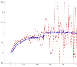
![Figure 4.2: Three simulations of the estimators of Buchmann and Gr¨ ubel [2003] (dashed red) and Coca [2015] (solid blue) for n = 1000](https://thumb-us.123doks.com/thumbv2/123dok_us/9905049.2483797/147.892.173.767.540.822/figure-simulations-estimators-buchmann-ubel-dashed-coca-solid.webp)
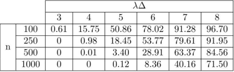
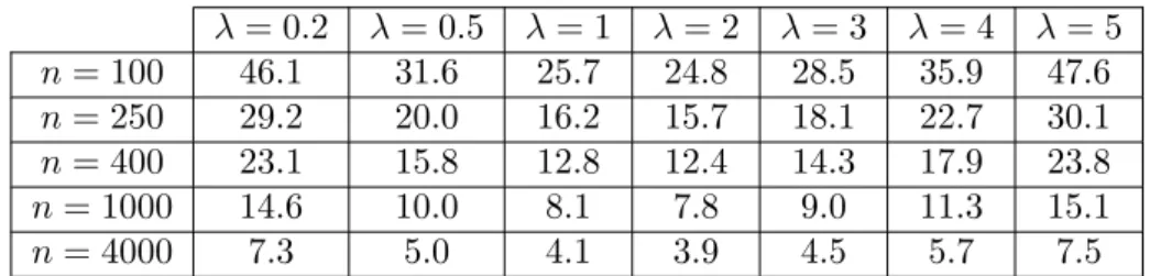
![Table 4.4: Average empirical 0.05-quantiles (coverage in %) from the estimators of Buchmann and Gr¨ ubel [2003] (B&G), Coca [2015] (C) and naive ones (N) under the respective norms and after 250 simulations with at least one zero-increment.](https://thumb-us.123doks.com/thumbv2/123dok_us/9905049.2483797/149.892.171.759.629.839/average-empirical-quantiles-estimators-buchmann-respective-simulations-increment.webp)
![Table 4.5: Average empirical 0.05-quantiles (coverage in %) from the estimators of Buchmann and Gr¨ ubel [2003] (B&G), Coca [2015] (C) and naive ones (N) under the respective norms and after 250 simulations with at least one zero-increment.](https://thumb-us.123doks.com/thumbv2/123dok_us/9905049.2483797/150.892.127.730.157.362/average-empirical-quantiles-estimators-buchmann-respective-simulations-increment.webp)
![Table 4.8: Average empirical 0.05-quantiles (coverage in %) from the estimators of Buchmann and Gr¨ ubel [2003] (B&G), Coca [2015] (C) and naive ones (N) under the respective norms and after 250 simulations with at least one zero-increment.](https://thumb-us.123doks.com/thumbv2/123dok_us/9905049.2483797/152.892.247.613.155.304/average-empirical-quantiles-estimators-buchmann-respective-simulations-increment.webp)
![Figure 4.5: Three simulations of the estimators of Buchmann and Gr¨ ubel [2003] (dashed red), Coca [2015] (solid blue) and the naive one (dashed-dotted green) for n = 400](https://thumb-us.123doks.com/thumbv2/123dok_us/9905049.2483797/154.892.145.725.555.839/figure-simulations-estimators-buchmann-dashed-coca-dashed-dotted.webp)
![Table 4.10: Average empirical 0.05-quantiles (coverage in %) from the estimators of Buchmann and Gr¨ ubel [2003] (B&G), Coca [2015] (C) and naive ones (N) after 250 simulations.](https://thumb-us.123doks.com/thumbv2/123dok_us/9905049.2483797/156.892.144.705.385.613/table-average-empirical-quantiles-coverage-estimators-buchmann-simulations.webp)
