An Evaluation of One Class Classifier on Gene Expression Data

(1)

AN EVALUATION OF ONE CLASS

CLASSIFIER ON GENE EXPRESSION DATA

Information Technology and Communication Science

Master’s Thesis

August 2019

(2)

ABSTRACT

Haifeng Xu: An Evaluation of One Class Classifier on Gene Expression Data Master’s Thesis

Tampere University

Master of Science (Technology) August 2019

It is not rare that medical data has imbalanced classes. This problem causes many difficulties when diagnosing rare diseases or cancer subtypes by machine learning tools, since traditional binary or multi-class classifiers lack the ability to classify imbalanced data. Therefore, One-Class Classifiers (OCC), the machine learning methods that only use data from one class, becomes one possible option. Our study evaluatesν-SVM, one of the most commonly used One-Class meth-ods, on four microarray datasets of Breast Cancer and Diffuse large B-cell lymphoma (DLBCL). Each cancer is labelled into different subtypes. We compared OCC with binary SVM and studied how the imbalance between the classes affects the results. The results show thatν-SVM performs better than binary SVM when the data classes are extremely imbalanced on these datasets. Keywords: Machine Learning, One-Class SVM, Bioinformatics, Microarray, Cancer Classification The originality of this thesis has been checked using the Turnitin OriginalityCheck service.

(3)

PREFACE

This thesis is written for the Master’s Degree in Science (Technology) of Tampere University. The thesis is about my personal research project supported by Medical Bioinformatics Centre, Turku Bioscience Centre, University of Turku and Åbo Akademi University.

Acknowledgements to Professor Tapio Elomaa, PhD, Tampere University, who has supervised this thesis. Thanks for his great advice about thesis writing. Acknowledgements to Adjunct Pro-fessor Laura Elo, PhD, University of Turku, the group leader of Medical Bioinformatics Centre, who has offered many guidances during the study. Acknowledgements to Post-doc Mikko Venäläinen, PhD, who guided me in the entire study with his knowledge and patience. Thanks to all the professors and teachers who taught me courses in Tampere University in the past three years. Tampere, 8th August 2019

(4)

LIST OF FIGURES

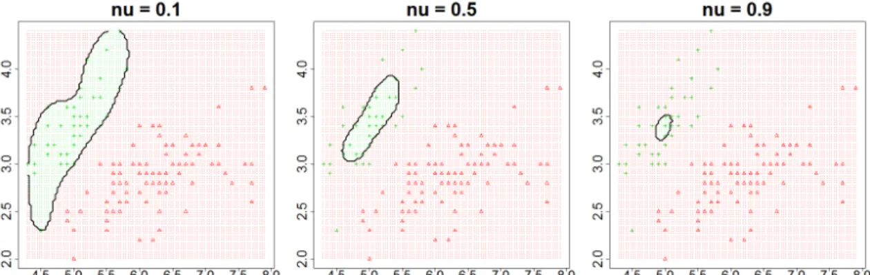
2.1 The effect of the parameterν. . . 7

2.2 A sample PCA plot on iris data. . . 9

2.3 Box plots of two genes expression. . . 10

2.4 DNA molecular structure. . . 11

2.5 An example of microarray data in RStudio environment (RMA normalized) . . . 12

2.6 Mammographies of a healthy person and a breast cancer patient. . . 14

2.7 Micrograph of a diffuse large B cell lymphoma . . . 15

3.1 A truncated gene table in R studio environment . . . 18

3.2 The overall workflow after the principal component analysis . . . 20

4.1 PCA plots for breast cancer data sets. . . 22

4.2 PCA plots for lymphoma data sets. . . 22

4.3 Kernel comparison results on breast cancer test data . . . 24

4.4 Kernel comparison results on lymphoma test data . . . 24

4.5 Results on breast cancer data (Reversed training and test sets) . . . 25

4.6 Results on lymphoma data (Reversed training and test sets) . . . 26

4.7 An example workflow of removing negative samples in the training set. . . 27

4.8 The imbalanced test results on breast cancer data . . . 27

4.9 The imbalanced test results on lymphoma data . . . 28

(6)

LIST OF TABLES

2.1 Confusion matrix . . . 8

3.1 Data sets used in this study. . . 17

4.1 The best parameters returned for the breast cancer data and the corresponding performances. . . 23

4.2 The best parameters returned for the lymphoma data and the corresponding per-formances. . . 23

4.3 The balanced accuracy of each kernel on the test sets. . . 23

4.4 The class ratio (Positive : Negative) of each training set. . . 28

(7)

LIST OF PROGRAMS AND ALGORITHMS

3.1 The R function that removes all low-expressed probes with replicated use . . . 18 A.1 the R code of parameter tuning function . . . 40

(8)

1 INTRODUCTION

Nowadays, pattern recognizing of medical data becomes very important because of the vig-orous increasing of data size. Among them, machine learning, a group of study about algorithms and statistical models, has shown more and more influence. Generally speaking, machine learn-ing is a method (or a group of methods), that allows one to build classification or regression models only by a pre-selected algorithm and the data itself. Since it does not require any explicit instructions from users, machine learning can usually find the hidden patterns that human cannot from the data.

Though it works well in many situations, there is still a serious problem when applying machine learning methods on medical data. In medical situations, it is very common that the two classes (patients vs healthy controls, or one subtype vs another) are not in balance. On one hand, prac-titioners cannot collect positive samples of rare diseases since they are not able to find patients. For example, a cancer may have 95% common subtype and 5% rare subtype, whose patients need special treatment. Due to the restriction of biological experiment (expensive and difficult to find volunteers), it is already difficult to collect data from the common subtype. As for the rare subtype, there could be only a few samples, or even less. On the other hand, for those common diseases with high diagnostic costs, it is not easy to collect negative samples either. For binary or multi-class machine learning methods, this is a challenge. In his review study, Khan shows that the performances of traditional multi-class classifiers suffer from the high imbalance between the classes [36].

Another problem with binary or multi-class classification methods is that they usually classify a new data point into one of the pre-defined categories [36]. But if a classifier tries to classify new samples from an entirely different domain, the results will always be wrong. For instance, imagine a multi-class model that was trained by cats, cows and pandas. What would happen if it tries to classify a car? It would return an animal category anyway, which is clearly wrong. In practice, a classification task is usually not to allocate new data points into several categories. Instead, the classifier should decide if this new data point belongs to a specific class or not [36].

All the problems above also frequently exist in medical studies. For instance, a cancer may have several subtypes but only one of them can achieve a high 5-year survival rate [69]. Ad-ditionally, there could be undiscovered subtypes. Therefore, if one wants to build a classifier to diagnose the "safe" subtype, one may need an approach that can learn the decision function only by the data of a single class. We expect this one-class approach can learn the decision boundary from the safe subtype, then can still determine if a new patient has any other "unsafe" subtype, even this subtype is unknown yet.

For above reasons, severalOne-Class Classification (OCC)methods have been developed in recent years. Comparing to binary approaches, OCC only requires data from the "interesting class". This allows for munificent savings in memory space and computation time, while keep-ing a comparable level of performance [61]. Among all OCC methods, Support Vector Machine based approaches (OSVM) have generated the most amount of applications. Because of their advancements, applicability, and the huge amount of applications, OSVM methods show their abilities that can be a separate research area in their own right [36]. The first OSVM approach, Support Vector Data Description (SVDD), was invented by Tax and Duin in 1999 [67]. Then in 2000, Schölkopf et al. published a new method,ν-SVM [59]. These two algorithms are compared and optimized in the past 20 years for several times. But in practice, they are usually used in text or documents classification. Only a few studies have applied OCC on medical data, such as applying on electroencephalography data, or MicroRNA of plants [23] [76]. Furthermore, only few studies applied OCC on gene expression data, although gene expression has been proved that it has a huge impact on many diseases. For example, certain genes are differentially expressed between multiple sclerosis patients and healthy people [35]. Therefore, it is potential to evaluate

(9)

how OCC works on gene expression data, in order to explore its clinical use.

In 2016, Sokolov et al. applied OCC on cancer subtype classification, which showed the potential use of OCC on gene expression data [63]. But some aspects in their study need more discussions. For instance, they evaluated the performance of OCC by Area under the Curve (AUC). However, AUC cannot distinguish which class contributes more to the overall performance [22]. They did not discuss the effect of imbalance either, although some studies have pointed out that the skewness between classes can influence the classification results [36] [22]. Therefore, the purpose of this study is to evaluate howone class classifier works ongene expression data, especially when the data classes are imbalanced. Furthermore, a proper evaluation standard is needed. We also try to explore if OCC is applicable on cancer subtype diagnosing.

For above purposes, in this study, both ν-SVM and binary SVM are evaluated on four mi-croarray datasets of two cancers, breast cancer and lymphoma. Each cancer has two labels, which are two different subtypes. For each cancer, we use one data set to train the classification models, and the other is for testing the performance. The training and test sets are uploaded on NCBI database by different organizations, which means these data sets are independent. Since they are independent, the performance would not be affected by experimental factors, such as the environment of laboratory or the operating habits of experimenters. We also have additional imbalanced tests to observe the influence of imbalance. In the imbalanced tests, the negative samples of the training set are randomly removed by 25%, 50%, 75%, and 90% respectively. Then we use the rest training samples to train the binary models, and compare their results with the performance of OCC.

In this study, we find that ν-SVM classifier has a comparable performance with binary SVM at the same level. When we remove negative samples from the training set, the performances of binary models reduce. The more negative samples we remove, the worse the binary models perform. Finally, the results of binary SVM become lower than OCC. Since OCC does not need negative data at all, it can be a better choice when the training set has only a few negative samples. We also discuss the possible threshold of the class ratio (Positive:Negatives) when OCC exceeds the binary models.

Chapter 2 of this thesis reviews the basic concept of OCC and other related studies. It also explains the concept of machine learning, basic mathematical expressions of the algorithms we use, and the related biology knowledge.

Chapter 3 introduces the methods and materials we use in this study. It includes the algorithm applications in R environment, the details of training and test data, the data pre-processing and feature selection, and the overall workflow.

Chapter 4 explains the results we have in this study, including the feature selection, kernel comparison and the imbalance test. It also discusses the limitation of this study, and the appro-priate circumstances to use OCC on gene expression data.

Chapter 5 gives the overall conclusion, the possible improvement, and the challenges of this study. A quick glance of this study is also give here.

(10)

2 THEORETICAL BACKGROUND

2.1 Related Work

The concept of OCC was mentioned for the first time in 1975 by Minter et al [46]. They proposed a classifier that only used data from "the class of interest". In the past 40 years, following terms were also used to describe OCC problems, such asSingle Class Classification[49],Outlier Detection [56], Concept Learning [29], and Novelty Detection [7]. In 2006, Juszczak defined One-Class Classifiers as"class descriptors that are able to learn restricted domains in a multi-dimensional pattern space using primarily just a positive set of examples"[55].

In his review study, Khan divides OCC methods into two categories [36]: 1 OSVM:Support Vector Machine (SVM) based one-class methods

2 Non-OSVM:including many one-class machine learning techniques based on random for-est, neural network, logistic regression, and others.

Although it seems unfair to regard SVM-based methods as an independent category, they do have shown that their advancements, applications, significance and difference, which made OSVM a separate research area [36].

As we mentioned in Chapter 1, the two main OSVM methods are SVDD and ν-SVM. The difference between them is how they separate the classes. SVDD constructs a hyper-sphere around the data, while ν-SVM creates a hyper-plane to separate the origin and the region that contains data [36]. These two algorithms are optimized for many times since they were first developed. In 2007, Yang and Madden optimized the CPU cost of parameter tuning forν-SVM [41]. They use particle swarm optimisation to calibrate the parameters. In 2010, a better decision function was improved by Tian and Gu based on the original function of Scholkopf [68]. As for SVDD, Luo et al., improved its accurateness by giving distinct costs to distinct system calls in 2007 [40]. In 2003, Mapping Convergence (MC) was presented by Yu et al. It is a one-class method that combines a weak classifier (as the first layer) and a SVM based classifier (as the second layer) [77]. The first layer is for extracting strong outliers that are very far from the positive class boundary. This gives MC better accuratenesses than other OSVM methods [77]. In next section, we will introduce the mathematical expressions of one of these two algorithms,ν-SVM.

Besides OSVM, there are also one-class methods based on other algorithms. In 2000, Manevitz and Yousef suggested a one-class neural network model, that filters documents by the objects from the "target class" only [43]. The problem with this neural network model is that it is sensitive with representation choices. In the same year, Letouzey et al. published a one-class decision tree [37]. But it is difficult to apply when the data has a high number of dimensions. The accuracy and robustness of this algorithm were improved by Li and Zhang in 2008 [38]. In 2001, Nearest Neighbours Description was proposed by Tax et al. It is a one-class k-nearest neighbours (kNN) algorithm, but with a defect that the model can become more sensitive to noise when increasing the amount of neighbours. One-class Bayes classifier was published much earlier. In 1997, Datta introduced a naive Bayes classifier with only samples from one class [17]. Wang also extent a one-class naive Bayes classifier in 2003 [71]. The newest one-class algorithm is the one-class logistic regression method suggested by Sokolov et al. in 2016 [63]. Other techniques include one-class anomaly detection, minimum spanning tree, and density estimator etc [62] [32] [26]. Although many special one-class methods were developed over the last 20 years, their authors still compare their performance with standard OSVM methods, since OSVM is still the most stable and applicable one-class algorithm [36].

OCC is not widely applied in bioinformatics research, although there are many medical data sets have unlabelled categories. Gardner et al. applied OCC on electroencephalography data in

(11)

2006 [23]. It shows the potential of combining OCC and biomedical data. OCC was also used to analysis multi-sequence magnetic resonance imaging (MRI) in 2015, in order to diagnosis multiple sclerosis lesions [34]. In 2016, Sokolov et al. presented the potential use of OCC on cancer diagnosis [63]. This is one the major study of applying OCC on gene expression data. They compared three main one-class machine learning methods,ν-SVM, SVDD, and one-class logistic regression [63]. The results show that ν-SVM and one-class logistic regression have similar performances on four microarray datasets, and they are always better than SVDD.

The literature review shows that there are not many applications about OCC on biomedical data, especially on gene expression data. Therefore, it is reasonable to evaluate the performance of OCC on gene expression data, in order to explore its possible use.

2.2 Mathematical Background

This section briefly introduces the basic concept of machine learning and mathematical terms used in this thesis. It is meant to explain these concepts to those reader without related back-grounds. It also gives the basic mathematical principles of the machine learning algorithms we use in this study:binary SVM andone-class SVM. Please notice that in this thesis, all vectors are denoted as bold letters, and the scalars are denoted as italic letters. For example,xdenotes an vector, butxdenotes a scalar.

2.2.1 Machine Learning

Machine learning, original proposed by Samuel in 1959, is an area of computer science that focuses on statistical models and algorithms [57]. It helps computers to do certain tasks without any specific programmed instructions. Instead, machine learning uses a certain algorithm to learn patterns and inferences from datasets. In his article, Samuel defined machine learning as "the field of study that gives computers the ability to learn without being explicitly programmed" [57].

We can have an example to make this concept clear. Think about the voice assistant on your smart phone and why it can understand the word you said. If we consider your voice as a signal, there are certainly many features that we can extract from it: frequency, amplitude, or the time you spent to pronounce. For different sentences, for instance, the voice of saying “yes” or “no”, these features are also different. Now if we have a dataset containing 1000 persons speaking “yes” and 1000 “no”, and simplify the features as frequency, amplitude, and time length, we will have a 2000x3 matrix in a 3-d space. Since the 3 features are all different between the 2 groups, the data points from different class should cluster at different positions, which means we can use a 2-d plane to separate them. Then a new data point without any label can also be classified by which side it falls on. There are many mathematical algorithms that we can calculate what this 2-d plane is, and all these algorithms require input data. In our case, it is the 2000x3 matrix. The whole process above is called machine learning, and we call the 2000x3 matrix as “training set”. In reality, it is usually more complicated than our example here. A high-dimension dataset like 3000-d is also quite common. Therefore, many different algorithms are given or optimized by practitioners to handle different types of problems, such as Convolutional Neural Network, Support Vector Machine, Random Forest, etc.

As an independent subject, machine learning developed rapidly over the last 20 years. From the 1990s, related researchers started to borrow mathematical models from statistics and prob-ability theories. Machine learning is also benefited by the development of Internet and computer hardware technologies. For example, we can use machine learning to analyse huge data sets nowadays because of the high-capacity disks and high-performance Central Processing Units (CPU).

Traditionally, machine learning tasks can be divided into two categories: supervised learning andunsupervised learning. In supervised learning, an algorithm needs labelled inputs (data) to build a mathematical model, then generates the outputs (class or value). According to the different outputs, we can divide supervised learning into classification and regression. When the outputs are discrete and limited labels, like our voice recognition model above, we call it classification. If the output is continuous, like predicting the temperature, we call it regression. Typical supervised learning methods include Support Vector Machine (SVM), Random Forests, Nearest Neighbours,

(12)

and Naive Bayes classifier.

In unsupervised learning, only unlabelled data is given to a machine learning algorithm. The algorithm need to find the structure of data, by grouping or clustering the data points. Unsuper-vised learning is usually used to discover the patterns in data. Typical unsuperUnsuper-vised learning methods include Neural Network, Cluster Analysis, Anomaly Detection, etc.

Machine learning is used in many applications. Nowadays, shopping websites and online me-dia use machine learning to learn the habits of users, then suggest commodities or programs that they are possibly interested. One of the most famous machine learning applications is "AlphaGo", an AI player developed by Google to play the board game Go . It used deep learning to learn how to play Go, and became famous after defeating many professional players. In 2017, it defeated Ke Jie, the number 1 ranked player in the world, which showed a huge potential use of deep learning in the field of artificial intelligence.

Although machine learning has achieved a huge success in various areas, it still has some limitations. One serious problem with machine learning is suffering from data biases. The outputs of machine learning models entirely depend on the training data inputted by human. Such bias can cause the inappropriate results, like racist and other presented unconscious biases [21]

2.2.2 Binary Support Vector Machine

Support Vector Machine (SVM) is a supervised machine learning method that can be applied both on regression and classification. The current standard version of SVM was invented by Vapnik and Cortes in 1995 [15]. Since then, it has been applied to many fields. The idea of SVM is characterized by its maximum margin property, or in other word, the decision boundary is chosen to be the one for which the margin is maximized [8].

The common two-class classification linear model can be described as follows:

y(x) =wTx+b, (2.1)

where x denotes an arbitrary vector in N-dimension space, b is the bias parameter, and the weightsware learned from the data. Therefore, we can get the corresponding decision boundary by following equation,y(x) = 0, which geometrically expressed as aN−1dimensions hyperplane. In 2-D case, it is a line orthogonal to the weight vector w. Then the classification rule can be written as:

F(x) = {︄

Class -1, ifwTx+b <0;

Class +1, ifwT_x₊_b_≥_0. (2.2)

For a pointxon the decision surface,y(x) = 0, according to the definition of dot product, we can have the distance from the origin to the decision surface:

wT_x

∥w∥ =−

b

∥w∥. (2.3)

According to equation (2.3), we can see that the bias parameterbdetermines where the decision surface locates in theN-dimension space.

Then we can have distance from an arbitrary pointxto the decision surface: r =y(x)/∥w∥. This can be got when we draw a vertical line to the decision surface. Now we can denote its orthogonal projection point onto the decision surface as x1. Since the vector from x to x1 is parallel to the weight vectorw, according to the definition of vector addition, we can have:

x=x1+r w

∥w∥. (2.4)

It is easy to solverby multiplying both sides of this equation bywT and addingb. According to y(x1) = 0and (2.1), we can solveras:

r=y(x)

∥w∥. (2.5)

It is common to write (2.1) as the following form when discussing SVM classifier:

(13)

whereφ(x) denotes a fixed feature-space transformation, and the training data set are usually defined as N input vectors x1, ... , xN, with corresponding target values t1, ... , tN, where

tn ∈ {−1,1}. The sign of y(x) can define the class of a new data point. If we assume that

the training data set is linearly separable in feature space, then there will be at least one set of parameter (w, b) exists. According to (2.2), for class -1, the parameter sets can givetn = +1for

all data points thaty(xn) > 0, andtn = +1for thosey(xn) < 0, so that for all the data points,

tny(xn)>0.

Often there are several parameter sets (w, b) exist, which means there could be several vec-tors in the feature space that can separate all the training points. Therefore, it is significant to find the best parameter sets that gives the smallest generalization error. From this perspective, the support vector machine is a method that solves this problem through the concept of the mar-gin, which is defined to be the smallest distance between the decision boundary and any of the samples [8].

From (2.4), we have the formula of distance from an arbitrary point to the decision surface, wherey(x)can takes the form of (2.6). Furthermore, the solution should satisfytny(xn)>0so

that it can classify all training points correctly. Therefore the distance can be given by following equation:

tny(xn)

∥w∥ =

tn(wTφ(x) +b)

∥w∥ . (2.7)

Thus the maximum margin solution of parameters set can be found by solving: arg max w,b {︃ ₁ ∥w∥minn [︂ tn(wTφ(x) +b) ]︂}︃ , (2.8)

and it can be simplified into an equivalent form [15]: arg min w,b 1 2∥w∥ subject totn(wTφ(x) +b)≥1, n={1,2, ..., N}. (2.9)

The solution of 2.8 can be gained by quadratic programming algorithm and Lagrange multi-pliers, and there are many tailored implementations exist [8]. The implementation of SVM used in this study is based on the used LibSVM library, a popular open SVM library developed at the National Taiwan University [12].

For all the procedures above, we assumed that all training samples are classified, but in reality we have to allow some samples to reside on the wrong side of the margin. Therefore, the penal-ization is introduced. For this purpose,w, b:x→f(x)=sgn(w·φ(x)−b)in chosen to minimize the resulting function.

The SVM solution can be extended to non-linear boundaries using the kernel trick. Essentially, it is a method that can map the data into a higher dimension, then design a linear SVM there. A basic kernel that maps 2D data into 3D can be described as(x, y)→(x, y,√2). which is called explicit polynomial kernel. This kernel can transform 2D data into 3D explicitly and fit the SVM with transformed data, but it is slow to compute. In practice, implicit mapping is much more popular. In implicit mapping, it substitutes each dot product in the SVM algorithm by the kernel κ(x,y) = (x,y)2_{and fits with original 2D data. This is the key to efficiency.}

There are many kernel functions for SVM. In our study, following kernels are tested for the both binary and OCC classifiers, then the kernel with the best performance was selected. Here lists the kernels that used in this study:

1 Radial Kernel: κ(x,y) = exp(︁

−∥x₂−_σ2y∥ )︁

; 2 Linear Kernel: κ(x,y) = (x·y);

3 Polynomial Kernel: κ(x,y) = (x·y)d;

(14)

Figure 2.1.The parameterν affects how many samples are included by the decision boundary

2.2.3 One-Class Support Vector Machine

ν-SVM is a one-class machine learning method proposed by Scholkopf et al [59]. Comparing with the binary SVM, we can get the determine function ofν-SVM,f(x), by solving the following equation: min w∈F,ξ∈Rl,b∈R 1 2∥w∥ 2₊ 1 νl ∑︂ i ξi−b subject to(w·φ(xi))≥b−ξi, ξi≥0, (2.10)

wherex1, ...,xl∈χare the data points of training data,l∈N is the observation times of training

data, andχ is a compact subset of RN. Letφbe a feature mapχ → F, i.e. a map into a dot

product space F such that the dot product in the image ofφ can be computed by evaluating a simple kernel, for example, radial kernel.

Like binary SVM, the solution of this algorithm can be gained by quadratic programming algo-rithm and Lagrange multipliers. It is shown in the original study of Scholkopf et al, so the specific proof process will not be explained in this thesis [59]. But it is still important to figure out one important parameter in this equation,ν.

When we have a new data pointx, we can determine the valuef(x)by judging which side of the hyperplane it falls on. Since non-zero slack variablesξiare penalized in the objective function,

and ifwandbare the solution of the equation above, the decision functionf(x)=sgn(w·φ(xi)−b)

will be positive for the most training pointsxi, while the SV type regularization term∥w∥will still be

small [59]. In this algorithm, the balance between these two goals is controlled by the parameter ν, furthermore, the parameter ν also characterizes the fractions of SVs and outliers [59]. Figure 2.1 shows the effect of the parameterν. As we can see the greater theνis, the less samples are included by the decision boundary. Therefore, it is the main parameter that we need to tune in this study.

2.2.4 Confusion Matrix and Balanced Accuracy

A confusion matrix is shown in Table 2.1. Traditionally, the termaccuracyis defined as(T++ F+_)/(T_+F_{). It represents the ratio of correctly predicted samples and all samples. Two important} statistical measures can be introduced here, sensitivity andspecificity. Sensitivity (true positive rate) measures the proportion of correctly identified positive samples, denoted as T+_/(T+ ₊ F−). Specificity (true negative rate), by contrast, measures the proportion of correctly identified negative samples, denoted asT−/(T−+F+_{). The balanced accuracy (BAR) is defined as the} average of sensitivity and specificity, which means it uses the information from the both sides [70].

(15)

Table 2.1.Confusion matrix

Object from positive class Object from negative class Classified into positive class True Positive,T+ _{False Positive,}_T− Classified into negative class False Negative,F− True Negative,F+

2.2.5 Principal Components Analysis

Principal Components Analysis (PCA) was invented by Pearson in 1901 [53]. As the name suggests, it is a statistic method that can extract the main components from all the features. PCA applies eigendecomposition on the covariance matrix, then obtains the principal components (i.e. eigenvectors, abbreviated to PC) of the data and their weights (i.e. eigenvalues). It is meant to explain the variance of original data, or in other words, which direction of the data value has the greatest influence on the variance.

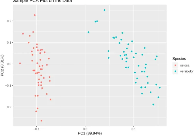
Generally, the results of principal components analyses are PCs. For the convenience of drawing plots, the typical number of PCs is two or three, though it can be technically more. As we introduced above, two PCs are two eigenvectors, which means we can draw a PCA plot by using PC1 as the x-axis and the PC2 as the y-axis. Figure 2.2 shows a sample PCA plot on an iris data set with two classes. There are four features in this dataset: sepal length, sepal width, petal length and petal width. We can see from the plot that these two classes are totally separated. The percentage after each PC represents how much variance this PC explains. If we add them up, the sum will represent the total percentage of variance that the PCA explains. If it is too low, the PCA may not explain the data set variance well. But if this percentage is high enough, it means what the plot shows is reliable.

PCA provides an effective way to reduce the data dimensions. It removes the components corresponding to the smallest eigenvalues in the original data, which means the low-dimensional data we get is optimized. In this study, we use PCA to evaluate our feature selection visually.

2.2.6 Basic Quartiles Terms and Box Plot

A box plot describes a group of numerical data by their quartiles and outliers. Before introduc-ing how to read a box plot, let us introduce the definitions of quartiles in statistics. First of all, we need to sort the current number list in the order of their values, from the lowest to the highest. Then the "median" is the number in the middle of the sorted list. If there are two numbers in the middle, the median is their mean value. Since the lower quartile (Q1) and the upper quartile (Q3) have several definitions, we only introduce the definition we use in this study.

If the data size is an odd number, we can use the median to divide the whole data set into two parts. The lower quartile (Q1) is the median of the lower half, and the upper quartile (Q3) is the median of the higher half. If the data size is an even number, divide the data into two parts with the same size. ThenQ1andQ3are the medians of these two parts. Interquartile Range (IQR), usually symbolized as∆Q, is defined as∆Q=Q3−Q1.

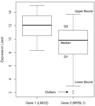
In a box plot, the upper bound of the data is defined as Q3 + 1.5∆Q, and the lower bound is defined as Q1−1.5∆Q. Any value greater than the upper bound or smaller than the lower bound is regarded asoutliers. Figure 2.3 shows the box plots of the expressions of two genes. For each box plot, the top and bottom of the box areQ3andQ1, and the band inside the box is the median. The whiskers represent the upper bound and the lower bound, and the outliers are plotted as small circles. We can see that the distributions between these two gene expressions are different. TheQ3of Gene 2 is even lower than the median of Gene 1. We can also know that the expression of Gene 2 has two outliers.

2.3 Biological Background

This section briefly introduces the basic biological terms used in this thesis. It is meant to explain them to readers without related backgrounds. It starts with the fundamental background

(16)

−0.2 −0.1 0.0 0.1 0.2 −0.1 0.0 0.1 PC1 (89.94%) PC2 (8.31%) Species setosa versicolor Sample PCA Plot on Iris Data

Figure 2.2. A sample PCA plot on iris data. The plot shows that these two classes are totally separated. We can see from the legends that PC1 and PC2 explain 97.71% data variance in total. This is a very high percentage, which means we can trust the what the plot shows to us.

of genetics: DNA, genes, gene expression, and what microarray data is. Then it explains the concept of cancer and the two diseases we studied.

2.3.1 DNA

The continuation of life depends on the hereditary information. It is passed from a cell to its daughter cell by the cell division, and passed to the next generation by its reproductive cells [2]. The most possible carrier element of hereditary information, deoxyribonucleic acid (DNA), was found in the 1940s. It stores these "genetic instructions" that determine the characteristics of species and each individuals [2].

The mechanism of DNA was not clear for a long time until its molecular structure was identi-fied by Francis Crick and James Watson in 1953. Generally speaking, a DNA is two long polynu-cleotide chains made from repeating units called nupolynu-cleotides [3]. The two chains bound to each other by hydrogen bonds and coiled around the same axis [73]. A DNA polymer can contain hundreds of millions of nucleotides, even though an individual nucleotide is quite small. After Crick and Watson, another possible carrier of hereditary information was found, ribonucleic acid (RNA). It carries the genetic information of many viruses. But since our study only focuses on Homo sapiens (or in more common words, human beings), and the genetic information of human is contained in DNA, we only introduce DNA and the related genetic processes in this chapter.

As the monomer units of DNA and RNA, nucleotides are organic molecules that have three distinctive chemical sub-units. Among them, the chemical sub-unit related to hereditary informa-tion is callednitrogenous base. In DNA, there are four bases found: adenine (A), cytosine (C), guanine (G), and thymine (T). Every single nucleotide has one of them. Nucleotides can pair with another on the other chain through their nitrogenous bases by the following rule: adenine -thymine and guanine - cytosine. This is usually symbolized as A-T and G-C base pairs [73]. The type of nucleotide is determined by its structure and nitrogenous base. Overall, there are thirty kinds of nucleotides. Fifteen of them belong to deoxyribonucleotide (unit of DNA), and the others

(17)

Upper Bound Lower Bound Outliers Q3 Q1 Median

Figure 2.3. Box plots of two genes expression. The top and bottom of the box are the higher quartile and the lower quartile, and the band inside the box is the median. The whiskers represent the upper bound and the lower bound. The outliers are plotted as small circles.

belong to ribonucleotide (unit of RNA). The hereditary information is hidden in the sequences of these nucleotides. For instance, different creatures can different nucleotide sequences in their DNA. Figure 2.4 shows the idealized straightened out DNA molecular structure and the double helix structure.

2.3.2 Genes and Gene Expression

In addition to DNA, the term "gene" is also widely used when discussing hereditary information. Generally speaking, a gene is the piece of a DNA, that could be able to produce a certain protein. In other words, a gene is a sequence of nucleotides in DNA or RNA with a specific function. These sequences are called codons, which behave like the "words" in the genetic "language". In his study, Pennisi defines genes as "any discrete locus of heritable, genomic sequence which affect an organism’s traits by being expressed as a functional product or by regulation of gene expression" [54].

A gene can have one or few names as its unique symbol to symbolize its function. These names are usually given by the HUGO Gene Nomenclature Committee (HGNC). In our study, all genes are described by their names.

The process of how genes affect human bodies is called "gene expression". It is a process that synthesizes functional gene products by hereditary information. In cells of Homo sapiens, this process is described by the "Central Dogma", which is usually stated as follows: "Transcription -Translation - Replication" or "DNA makes RNA and RNA makes protein" [16].

(18)

Figure 2.4.The idealized straightened out DNA molecular structure is shown on the left, and the right part shows the double helix structure of DNA [2]

The production of transcription is a RNA chain. It copies the hereditary information from the DNA. As a single chain of nucleotides, a RNA chain is synthesized by pairing nucleotides with DNA, just like one DNA chain pairs with another. The only difference is the thymines (T) in DNA are replaced with uracils (U) in RNA (symbolized as A-U and G-C). During the transcription, a gene on DNA will be read and copied to messenger RNA (mRNA). After editing and splicing, each mRNA will get close to ribosome to start the translation. The product of translation is protein. For Homo sapiens, it is the final product of gene expression.

Measuring gene expression products is quite important to modern medical study. For exam-ple, Zhao et al. has discovered that lymphoma patients with different lymphoma subtypes can have different expression level on certain genes [80]. Therefore, in order to classify the cancers subtypes, it is reasonable to use gene expression level to build the machine learning models.

2.3.3 Microarray Data

DNA microarray, firstly invented in 1983, is the most commonly used tool to measure gene expression product. Over the past 40 years, it is used to measure the expression level of a large number of genes [65]. As we mentioned in last subsection, the product of gene expression can be either mRNA or protein. However, microarray only measures one of them, which is mRNA. This is because the principle of microarray technique is based on the complementary property of nucleotides.

The principle of microarray technique can be generally stated as follows: the hybridization be-tween one DNA strand and mRNA, or in other words, the complementary property of nitrogenous base pairs. In practice, a microarray chip is a solid surface with microscopic DNA spots on it. These DNA spots are called "probes". These probes can hybridize the mRNA in expression prod-uct sample, then generate fluorescent or electric signal. Microarray can compare the strength of these signals by using relative quantification and thereby measure the expression level of each gene.

(19)

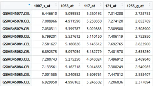
Figure 2.5.An example of microarray data in RStudio environment (RMA normalized)

synthesizing a short sequence, or a reverse transcription from mRNA to cDNA. The second way utilizes the complementary property of nitrogenous bases we mentioned above (A-U, G-C).

In practice, a probe is shorter than a gene. For Affymetrix array, a famous microarray brand, each target gene is represented by a probe set that contains 11 to 20 probe-pairs [50]. Each probe pair is combined by one Perfect Match (PM) probe and one MisMatch (MM) probe. A PM is a probe that is perfectly complementary to the target, while a MM is a probe whose central base is mismatched [50]. Generally, MM probes are used to measure the amount of non-specific bindings. Often there are tens of thousands probe sets in a microarray dataset. Figure 2.5 shows a microarray dataset in RStudio environment. The row names are the sample ids on NCBI database, and the column names are the probe sets ids.

Because of the existence of MM probes, it is important to do normalization when analysing microarray data. One common method of normalization is Robust Multi-array Average (RMA) [28]. However, it only summarizes the perfect matches and mismatch spots are not utilized. The Median Polish Algorithm is used in RMA method of summarizing the information from perfect matches [24]. This is a robust exploratory data analysis procedure proposed by John Tukey in 1977. It it is meant to find an additively-fit model for two-way layout data by its row effect, column effect, and overall effect [48]. The general description of Median Polish Algorithm can be explained as follows:

1. Find theoverall effect: put all medians of each row in a vector, and find the median of this vector;

2. Each element in the first row minuses the median of this row, then repeat this for each row;

3. Subtract the overall effect from each row median;

4. Do the same thing to each column, and add the overall effect from column to the add the overall effect that was received before;

5. Repeat steps 1 - 4 until very insignificant change occurs with row or column medians. There are also other components in RMA normalization, such as quantile normalization, a method of normalizing a batch of arrays, and log-2 transformation. These procedures make the magnitudes of data at a comparable level for each the probe set and sample.

2.3.4 GEO and NCBI

GEO is the abbreviation of Gene Expression Omnibus, one of the largest public databases of high-throughput data. It also includes the information about related chips, microarray, RNA

(20)

sequences, and other similar data types [14]. It provides tools for users so that they can download and analysis the data. The GEO databases are supported by National Center for Biotechnology Information (NCBI).

2.3.5 Cancer

Cancer is the combination of a group of diseases, caused by abnormal cells that keep un-stoppable divisions in the lesion. Normally, programmed cell death is a regular process in human bodies. Cells die when they get damaged or become old. In biological term, this is called apopto-sis. However, the abnormal cells of cancer tumours survive even when they are old or damaged, and new cells are still generated when they are not needed. The abnormal cells can spread to surrounding organs and tissues, then result in their death. Finally, it leads to the death of patients. Cancer is the main reason why mortality happens on human beings. In 2012, cancer caused around 8 million death worldwide. Meanwhile, approximately 14 million new cases happened in the same year [64].

There are many risk factors that may cause cancers, such as tobacco use, obesity, ionizing radiation, environmental pollutants, and lacking physical activity. Alcohol intake was also find as a major cause of cancers [39]. Infections of microbes such as Helicobacter pylori, human papillomavirus infection, and human immunodeficiency virus (HIV) are also the main reasons why cancers happen, especially in developing countries. Beside above, an unavoidable risk factor of cancer is the genetic reason. It has been proved that all cancers happen with genome mutations [64]. It means that the encodes of some genes are permanently changed in the DNA sequence. Furthermore, some genes can differentially express between cancer patients and healthy people, which means it is potential to used gene expression data to do cancer classifications [1].

There are various of criterion to divide a cancer into subtypes. Clinically, it is common to do it by different treatment effects, e.g. the five-year survival rate. Five-year survival rate is one option to evaluate how the therapies work, especially on those aggressive diseases with a shorter life expectancy following, for example, the lung cancer. Two subtypes of one cancer may react differently to the same medicine, which may lead to different five-year survival rates. Nowadays, molecular subtypes are also often used on cancer classification because of the development of gene-targeted therapies. For example, there are two molecular subtypes of the basal bladder cancers, "epithelial" and "mesenchymal" [44]. Though the criterion of molecular subtypes still focuses on the survival rate, it gives more specific explanation in the aspect of molecular biology. Therefore, it is more popular in recent studies.

2.3.6 Breast Cancer

Breast cancer is a cancer that develops from breast tissue, accounting for 25% of all cancer cases [64]. It happens 100 times more often in women than men, which make itself the leading type of cancer in women worldwide. Usually, a patient will find a lump in the breast tissue or under armpits, that different from the other parts of the breast. Other symptoms includes the shape or position changing of the nipples, and the pain under armpits or around the collarbone [74]. Figure 2.6 shows the mammographies of a healthy breast (left) and a breast with breast cancer.

The risk factors include environmental and hereditary factors. Among them, the preventable environmental factors, such as alcohol intake, fat gain, lacking exercise, ionizing radiation, and chemicals, cause approximately 70% of the cases [42]. The other 30% of the cases are caused by the hereditary factors, which are usually non-preventable, for instance, genetic reasons. There are two high-risk genes identified, BRCA1 and BRCA2, that cause the most familial predisposition cases [64]. Besides, the expression of estrogen receptors (ER) and progesterone receptors (PR), and the over-expression of human epidermal growth factor receptor 2 (HER2) protein are also three main reasons why breast cancer occurs [6] [64]. Receptors are certain kinds of protein molecules that can receive chemical messengers, like hormones, from outside a cell. Breast cancer cells may have these receptors on their surface, cytoplasm or nucleus.

The biological reason why receptors can cause breast cancer is still not clear. In 2006, Deroo et al. proposed two hypotheses of the relationship between ER and breast cancer. The first hypothesis is that mutations happen when estrogen binds to ER. It stimulates the proliferation of

(21)

Figure 2.6.Mammographies of a healthy person (left) and a breast cancer patient [5].

mammary cells, since this process increases in cell division and DNA replication [18]. Moreover, estrogen metabolism can produce genotoxic waste, which may also increase the risk of breast cancer [18].

Clinically, it is very important to know if a receptor exists in the cancer cells. If breast cancer cells have ER receptors (usually called ER positive or ER+), the growth of these cells depends on estrogen. Then we can make the cancer cells necrosis by applying drugs that block estrogen effects. Therefore, it is reasonable to classify breast cancer by three following ways: ER positive or negative, PR positive or negative, and HER2 positive or negative. In our study, we divided breast caners into ER+ subtype and ER- subtype, then used them as the two classes of machine learning models.

2.3.7 Diffuse Large B-cell Lymphoma

Lymphoma is a kind of haematological malignancy, or generally speaking, a blood cancer. Worldwide, lymphoma has become the seventh most common form of cancer in the term of "can-cer incidence" [64]. In 2012, there were around 566000 new cases of lymphoma and 305000 deaths caused [64]. Symptoms can be found on early stage patients, including enlarged lymph nodes without pain, fever, night sweats, weight loss, and tiredness.

Traditionally, lymphoma can be classified into two main categories: Hodgkin’s lymphoma (HL) and non-Hodgkin lymphoma (NHL). Recently, the World Health Organization (WHO) added two new subtypes, which are multiple myeloma and immunoproliferative diseases [64]. As the name suggests, non-Hodgkin lymphoma (NHL) includes all types of lymphoma other than the Hodgkin’s. Comparing with non-Hodgkin lymphoma, Hodgkin’s lymphomas patients can have much better treatment effects. For those patients who are under 20-year old, the 5-year survival rates are around 97% [31]. However, for non-Hodgkin’s lymphoma patients, it is only around 71% [60]. In our study, we use the data ofDiffuse Large B-cell Lymphoma (DLBCL), a subtype of non-Hodgkin lymphomas. It is the most common subtype that accounts for 40% of lymphoma cases worldwide [64]. Figure 2.7 shows the micrograph of diffuse large B cell lymphoma.

The causes of DLBCL are still not clear, but there are some hypotheses, such as underlying immunodeficiency and the infection of Epstein–Barr virus (EBV) [52]. Genetically, it is found by Morin et al., that genes with candidate mutations are ubiquitous in DLBCL patients [47]. Further-more, a recent genome-wide association study of B cell non-Hodgkin lymphoma reveals that 3q27 is identified as a susceptibility locus in the Chinese population [33].

(22)

Figure 2.7.Micrograph of a diffuse large B cell lymphoma [51].

In 2012, Care et al divided DLBCL into three subtypes: germinal centre B-cell like (GCB), activated B- cell like (ABC), and unclassified (UC) subtype [9]. It is reported by Tirado et al that GCB patients have a much higher 5-year survive rate (59%) than ABC patients(30%) [69]. Moreover, the study of Zhao et al showed that there are eight significant genes that are related to the subtype formation [80]. Based on these studies, we think it is potential to build a classification machine learning model of DLBCL subtypes.

It is worth to mention that the unclassified subtype is not an independent subtype. Instead, it includes cases between ABC and GCB that cannot be clearly classified [80]. Clinically, it is much important to find those patients who have more dangerous subtype, in order to give them special treatments. In our case, it means we can regard GCB as the "safe" subtype, and all non-GCB subtypes as the "dangerous" subtype. Therefore, we divide all the patients into two groups, GCB and non-GCB, then build classification models based on these two classes.

(23)

3 MATERIALS AND METHODS

In this study, we evaluated two algorithms,ν-SVM and binary SVM. This chapter will introduce the materials and the R applications we use, how we do the data pre-processing, and the overall workflow.

3.1 Algorithm Applications

In Chapter 2, we saw that OSVM is much more applicable and stable than other one-class methods. Hence, we did not choose any one-class methods other than OSVM. In this study, two OSVM methods were considered at the beginning,ν-SVM and SVDD [66] [59]. But as we men-tioned in Chapter 2,ν-SVM achieves much better results than SVDD in the research of Sokolov et al [63]. Thus, we selectν-SVM classifier as the OCC machine learning method, and compare its performance with the standard binary SVM classifier.

Because OCC classifiers are commonly used on imbalanced data, it is inappropriate to use "accuracy" as the criterion to evaluate an algorithm. In imbalanced data, one class often has much more samples than the other. A classier may achieve very high performance when identifying the major class, but has very low ability to detect the minority class samples. Therefore, in this case, it is still not a proper classifier to detect the outliers. In order to solve this problem, Villalba et al. introducedbalanced accuracy (BAR) to evaluate OCC algorithms [70]. The BAR is defined as the average of the true positive rate (sensitivity) and true negative rate (specificity) [70]. For more details about the definition of BAR, see Chapter 2. In this study, we use BAR as the criterion of all machine leaning models.

The machine learning application we use is the R Package "e1071", developed by Meyer et al. It focuses on short time Fourier transform, fuzzy clustering, support vector machines, and other statistics methods [45]. We use the "svm" function of this package to build the machine learning models. The one-class SVM algorithm in this package is theν-SVM as we described in Chapter 2, and the binary SVM is the standard SVM algorithm. The evaluation function "ConfusionMatrix" is a built-in function of the package "caret" [30]. It gives the confusion matrix by the prediction and the test labels. We can get the BAR directly from the function output.

3.2 Training Data and Validation Data

All data sets we use in this study are microarray data. As we mentioned in Chapter 2, microar-ray contains the information of gene expression level. The changing of gene expression level may indicate a disease happens, or the difference between subtypes [25]. The normalized data of the two cancers are directly downloaded from Gene Expression Omnibus (GEO) database.

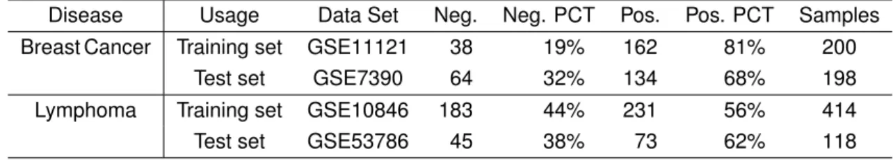
For the breast cancer experiment, a group of 200 patients from GSE11121 is treated as train-ing set and a group of 198 patients from GSE7390 is the test set [58]. Each data set is divided into the two groups we introduced in Chapter 2: ER positive and ER negative. Comparing to ER negative patients, an ER positive patient usually has a better survival prognoses [13]. In the experiment of lymphoma, a group of 414 patients from GSE10846 are treated as training set and a group of 118 patients from GSE53786 are as the test set. The original data has three subtype labels: GCB, ABC, and unclassified (UC) [80]. As we see in Chapter 2, GCB lymphoma patients has really high 5-year survival rates comparing with other subtypes [69]. Therefore, we combine ABC and UC subtypes as the "Non-GCB" subtype, and the data is manually labelled into two groups: GCB and Non-GCB.

(24)

Table 3.1.Data sets used in this study.

Disease Usage Data Set Neg. Neg. PCT Pos. Pos. PCT Samples

Breast Cancer Training set GSE11121 38 19% 162 81% 200

Test set GSE7390 64 32% 134 68% 198

Lymphoma Training set GSE10846 183 44% 231 56% 414

Test set GSE53786 45 38% 73 62% 118

on external data sets. The main reason why we did not choose cross-validation is the effect of the instrumentation or procedures. Experimenters may make mistakes when doing the experiment, and these mistakes may repeat during the whole experiment. The environment of laboratories can also affect the results, for instance, the temperature. Using an independent data set as the test set can avoid the interference above, because different contributors can hardly make the same mistake in the experiments.

Table 3.1 lists the data sets we use. In this study, we call the class with more sample points as themajor class, and the other class as theminority class. In order to make OCC classifier to have better performance, we use the major class as the OCC training set. The major class is labelled as positive or 1, while the minority class is labelled as negative or 0. In breast cancer data sets, the positive class is the ER+ subtype. In lymphoma datasets, it is the Non-GCB subtype. We use the entire training sets to train the binary model, but only the positive class is used to train the OCC models.

3.3 Data Pre-processing

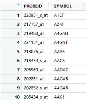
As described in Chapter 2, the downloaded microarray data is with probe ids as its rows, and sample ids as its columns. Therefore, our first step is converting probe ids to gene names, then we can select the gene we want. It is worth to mention that one probe may point at sev-eral genes in microarray data. Since these probes cannot give the expression level of a certain gene, we cannot use them as features. Therefore, we delete these probes before analysing. The annotation from probes to genes can be done by the annotation function. This is provided by the microarray platforms. In our study, the data sets are generated by following microarray plat-forms: [HG-U133A] Affymetrix Human Genome U133A Array and [HG-U133_Plus_2] Affymetrix Human Genome U133 Plus 2.0 Array [10] [11]. So we download the corresponding packages, "hgu133a.db" and "hgu133plus2.db", to apply the annotations. The data sets are also transposed to suit the requirement of the machine learning application. The following R commands can an-notate probe ids to gene names:

probe = colnames(microarray_data)

gene_table = AnnotationDbi::select(hgu133plus2.db,keys=probe,columns=c("SYMBOL"))

As a major input, the variable "columns" contains the column names of the transposed data, which are the probe ids. The code returns a gene table. Figure 3.1 shows a truncated gene table in R studio environment, whose first column, "PROBEID", contains probe ids, and the second, "SYMBOL", contains the gene names. If one probe points at several genes, the "SYMBOL" of this probe id will be empty. In this study, they are deleted before analysing.

Moreover, a microarray dataset may contain several probes that map the same gene. A com-mon way to compare them is to keep the probe with the highest median value, and remove the other [72]. Since there are around 20000 probes in a dataset, we write a small function to clean the replicate probes automatically. Program 3.1 shows the R code of this function, where the data must be a transposed microarray matrix.

After annotation, the data is labelled into positive or negative groups by their metadata. Since the downloaded data is already normalized by RMA method, no more normalization is needed.

(25)

Figure 3.1.A truncated gene table in R studio environment

1 ####### compare d i f f e r e n t probes w i t h t h e same gene ####### 2 # s o r t t h e gene_t a b l e by gene name b e f o r e t h i s f u n c t i o n 3 gene_median_comparison <− f u n c t i o n(data, gene_ t a b l e) {

4 maxium = 1

5 marker = matrix( 0 ,nrow( gene_ t a b l e) , 1 ) 6 marker [ maxium ] = 1

7 i = 2

8 f o r ( i i n 2 :nrow( gene_ t a b l e) ) {

9 i f( gene_ t a b l e $SYMBOL[ i ] == gene_ t a b l e $SYMBOL[ i −1 ] ) { 10 i f(median(data[ , gene_ t a b l e $PROBEID [ i ] ] )

11 > median(data[ , gene_ t a b l e $PROBEID [ maxium ] ] ) ) {

12 marker [ i ] = 1 13 marker [ maxium ] = 0 14 maxium = i 15 }else{ 16 next( ) 17 } 18 }else{ 19 maxium = i 20 marker [ maxium ] = 1 21 } 22 }

23 gene_ t a b l e = cbind( marker , gene_ t a b l e)

24 gene_ t a b l e = gene_ t a b l e[ gene_ t a b l e $marker == 1 , ] 25 r e t u r n( gene_ t a b l e)

26 }

(26)

3.4 Feature Selection

Some studies have indicated that breast cancer and DLBCL are highly associated with the expression of certain genes. Therefore, we select features based on these studies. It is reported by Wirapati et al., that the following seven genes are related to the formation of breast cancer tumours: AURKA, PLAU, STAT1, VEGF, CASP3, ESR1, and ERBB2 [75]. Particularly, ESR1 represents the ER signalling. Therefore, all the genes above are used to build the machine learning model. As for DLBCL, Zhao et al. introduce that the following eight genes are related to the subtype conformation: MYBL1, LMO2, BCL6, MME, IRF4, NFKBIZ, PDE4B, and SLA. These genes express differently in the patients of Non-GCB and GCB subtypes, which made themselves expectable features [80]. In order to see if potentiality of these features, we apply Principal Component Analysis (PCA)on all the datasets after feature selection.

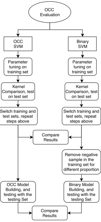
3.5 Work flow

This section briefly explains the workflow after PCA. The data of each disease will be evaluated by the following procedures.

First, since there are four kernels for both binary and OCC classifier, we need to compare the performance of each kernel. For both diseases, we tuned parameters for each kernel by a 10-fold cross-validation in the training set. Then we select the best parameters of each kernel, build models with them, and test these models on the test sets. The results are compared with their BAR. Furthermore, since the parameter tuning may cause over-fitting, we reversed the training and test sets, then did the tests again. The workflow of reversed tests are the same as the normal tests.

There are some studies that indicate the performance of OSVM is better than binary SVM when only few negative samples exist [36]. Therefore, we applied imbalanced tests to see if OCC works better when we remove some negative samples. For each disease, we remove certain proportion of negative samples in the training sets in the following order: 25%, 50%, 75%, and 90%. Before each removal, the negative samples in the training set are sorted into a random order to keep the results more stable. Then we use the rest of the training data to build the binary models. For each percentage, the operation above is repeated for 10 times.

See Figure 3.2 for the overall work flow of this study. The replicated operations, like removing negative samples, are drawn only once.

(27)

OCC Evaluation OCC SVM Binary SVM Parameter tuning on training set Kernel Comparison, test on test set

Switch training and test sets, repeat

steps above Parameter tuning on training set Kernel Comparison, test on test set Compare Results Remove negative sample in the training set for different proportion

Compare Results OCC Model

Building, and testing with the

testing Set

Binary Model Building, and testing with the

testing Set Switch training and

test sets, repeat steps above

(28)

4 RESULTS AND DISCUSSION

4.1 Results

After all the pre-processing steps, such as labelling, annotation, and feature selection, the datasets are checked by PCA. The purpose of PCA is to see if the features are selected success-fully. Figures 4.1 and 4.2 show the PCA plots of all the data sets we use.

We can see from Figure 4.1 that the two classes of breast cancer are generally separable, both in the training and test set. Thus, it is possible to use these features to classify the ER+ and ER- subtypes. This result verifies the biological meaning of our predefined classes, that is, these genes differentially expressed between ER+ and ER- breast cancer patients. As for lymphoma data, we plot their PCA by their original labels, which are GCB, ABC and Unclassified. As we presented in Chapter 2, GCB patients have much higher 5-year survive rates after treatments, so it is better to divide the dataset into GCB (relatively safe) and non-GCB subsets (the combination of ABC and unclassified class, possibly dangerous). The PCA plots of lymphoma datasets sup-port our division in another aspect. In Figure 4.2, we can see that the unclassified data points are between GCB and ABC. This supports the theory we mentioned in Chapter 2, that is, the unclas-sified subtype is not an independent subtype, but some unclear patients between GCB and ABC subtypes. Therefore, it is reasonable to combine ABC and unclassified classes as a single class, then compare it with GCB group. Furthermore, the PCA plots show that our feature selection of lymphoma data is successful since the classes are separated in these plots.

The machine learning models in this study are built in R environment. In Figure 2.1, we showed that the parameterν has a huge impact on OCC SVM boundaries. Another important parameter, γ, decides how many support vectors there are. The larger ourγ is, the fewer support vectors we have. A hugeγmay cause the models only work surrounding the training points, so it is also an important parameter for both OCC and binary SVM. Therefore, it is necessary to tune these parameters before each SVM model builds. Appendix A shows our parameter tuning function in R codes. A parameter set ofν (0< ν <1) is given to the function, and a parameter set ofγ, too. In order to avoid using information from the test sets, the parameter tuning is done by a 10-fold cross-validation within thetraining set. The polynomial kernel is tuned independently because it needs an additional parameter set,degree. Since we compare all kernels and many possible parameter values are tested, there are too many tuning results generated. Therefore, we only show the parameter combinations that give the best tuning results in Table 4.1 and 4.2. They also give the corresponding balanced accuracies. After comparing, the best kernel for breast cancer models is the sigmoid kernel, and the best kernel for lymphoma models is the radial kernel.

In Figure 3.2 and Chapter 2 we showed that it is important to select the best kernel for each classifier. In this study, all major kernels are compared: radial, liner, polynomial, and sigmoid. Since we have already gotten the best parameter sets for each kernel from parameter tuning, we can now build a model for each kernel by using the corresponding parameters. The results of kernel selection are shown in Figure 4.3 and Figure 4.4.

In Figure 4.3, we observe that the sigmoid and radial kernels have much higher performances than the other two kernels. Moreover, the balanced accuracies of these two kernels are both over 0.8. These results show expectable prospects of the classification. The kernel comparison in the lymphoma data sets return similar results, but only the radial kernel gives a high BAR for OCC-SVM. The specific BARs are listed in Table 4.3.

We can see from the plots that the best kernel for breast cancer models is the sigmoid kernel, while the best for lymphoma models is the radial kernel. Remind that we get these results on the external test sets, and they are the same as the best kernels we get from parameter tuning (cross-validation). For above reasons, we only use these two kernels in the following imbalance study.

(29)

Figure 4.1. PCA plots for breast cancer data sets. The blue points represent estrogen recep-tor(ER) positive samples, and the red points stand for ER negative samples. It is clear that the two classes clustered on different parts of the plots, so that it is potential to use our features to build a machine learning model.

Figure 4.2. PCA plots for lymphoma data sets. The red points represent ABC subtype samples, the green points stand for GCB subtype samples, and the blue points stand for unclassified sam-ples. We can see from the figure that the ABC and GCB subtype clustered on different parts of the plots. Also the unclassified samples clustered in between with ABC and GCB, which explained why we can combine it with ABC as the "Non-GCB" subtype. It shows that it is potential to use our features to build a classification model.

(30)

Table 4.1.This table shows the best parameters for thebreast cancerdata and the correspond-ing balanced accuracies. The input vector of parameterν is {0.005, 0.1, 0.2, ..., 0.9, 0.995}. The γset is 1 / (1, 2, ..., 1000). For each kernel, we did a 10-fold cross-validation in the training set, then used the mean value of the BARs as the performance. Here we only show the parameter combinations that give the best tuning results. We can see from the table that the best kernel for breast cancer data is the sigmoid kernel.

Classifier Outputs Linear Radial Polynomial Sigmoid

OCC Performance 0.640 0.873 0.531 0.890

ν 0.5 0.005 0.1 0.2

γ N/A 1/32 1/7 1/25

degree N/A N/A 3 N/A

Binary Performance 0.926 0.923 0.868 0.933

γ N/A 1/15 1/8 1/9

Table 4.2. This table shows the best parameters for thelymphomadata and the corresponding balanced accuracies. The input vector of parameterν is {0.005, 0.1, 0.2, ..., 0.9, 0.995}. Theγ set is 1 / (1, 2, ..., 1000). For each kernel, we did a 10-fold cross-validation in the training set, then used the mean value of the BARs as the performance. Here we only show the parameter combinations that give the best tuning results. We can see from the table that the best kernel for lymphoma data is the radial kernel.

Classifier Outputs Linear Radial Polynomial Sigmoid

OCC Performance 0.573 0.792 0.624 0.531

ν 0.8 0.1 0.005 0.1

γ N/A 1/26 1 1/49

Binary Performance 0.901 0.910 0.890 0.902

γ N/A 1/26 1/4 1/12

Table 4.3. The balanced accuracy of each kernel on thetest sets. The comparison shows that the best kernel for breast cancer data is sigmoid kernel, and for lymphoma, it is radial kernel. On the same disease data, the best kernels are the same for both OCC SVM and binary SVM.

Disease Classifier Radial Linear Polynomial Sigmoid

Breast Cancer OCC 0.818 0.389 0.590 0.859

Binary 0.873 0.861 0.875 0.876

Lymphoma OCC 0.881 0.686 0.754 0.678

(31)

Figure 4.3. Kernel selection results on the breast cancer test set. The blue bars represent OCC performances, and the pink bars represent for the binary classifier. The performances are evaluated by balanced accuracy. The binary classifiers with different kernels achieve similar per-formances. But only sigmoid and radial kernels give a good performance for the OCC classifier (BAR > 80%). The figure shows that sigmoid kernel is the best kernel on breast cancer data for both classifiers, OCC and binary.

Figure 4.4. Kernel selection results on the lymphomatest set. The blue bars represent OCC performance, and the pink bars represent for the binary classifier. The performances are evalu-ated by balanced accuracy. The figure shows that Radial kernel is the best kernel on lymphoma data for both OCC and binary classifiers.