Cloud Capacity Management

Cloud Capacity Management

This chapter provides a detailed overview of how Infrastructure as a Service (IaaS) capaci-ty can be measured and managed. Upon completing this chapter, you will be able to understand the following:

■ The basic challenges and requirements for managing capacity in an IaaS platform

■ How to model and manage capacity

■ The importance of demand management

■ The role of the procurement process in cloud

Tetris and the Cloud

As discussed throughout this book, the cloud consumer views the cloud as an infinite set of resources that it can consume as required. This clearly is not the case from the provider’s point of view, nor is it a sustainable business model. So, the cloud provider (either an IT department or telco) must provide the illusion of infinite resources while con-tinually optimizing and growing the underlying cloud platform in line with capital expen-diture (CAPEX) and service-level agreement (SLA) targets. There is often debate within IT organizations as to whether a formal capacity management process is needed, as hardware costs have continued to fall. This is based on the premise that capacity management is purely a CAPEX management function; however, with the introduction of the cloud, capacity management also becomes an SLA management function. This stems from the possibility of SLA breaches because of oversubscribed equipment or lack of resources to support the bursting of existing services or the instantiation of new services, which will inversely impact the user experience of a cloud service. The self-service nature of the cloud and the increase in virtualization and automation make capacity management more complex as providers can no longer over dimension their infrastructure to support peak usage, as peak usage will vary dramatically based on consumer requirements. To visualize this, think of a typical data center as the game Tetris, as illustrated in Figure 12-1.

New Workload Requirement Capacity Management Existing Workload Bursting POD POD Figure 12-1 Tetris

A finite number of colored shapes (workloads) fall down into a clearly defined area (infra-structure point of delivery [POD]), and the position and orientation of the shape are opti-mized to fit that area. If the optimization process is successful, more shapes fall down; if not, they build up and until they fill the hole. Now, increase the speed and have an infi-nite number of shapes and colors (as workloads will have different resource dimensions), and you have a true cloud. Somewhere in the middle will be the cloud that is available today from most providers. There aren’t an infinite number of workloads, but the demand is still much higher.

Capacity management, as defined by Information Technology Infrastructure Library Version 3 (ITIL V3), is seen as an ongoing process that starts in service strategy with an understanding of what is needed and then evolves into a process of designing capacity man-agement into the services, ensuring that all capacity gates have been met before the service is operational, and finally managing and optimizing the capacity throughout the service life-time. You can view capacity management as the process of balancing supply against a demand from a number of different dimensions, the main two being cost and SLA.

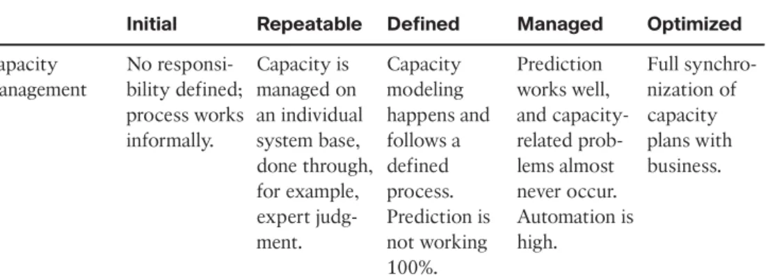
Table 12-1 Capacity Management Maturity (Forrester)

Initial Repeatable Defined Managed Optimized

Capacity management No responsi-bility defined; process works informally. Capacity is managed on an individual system base, done through, for example, expert judg-ment. Capacity modeling happens and follows a defined process. Prediction is not working 100%. Prediction works well, and capacity-related prob-lems almost never occur. Automation is high. Full synchro-nization of capacity plans with business. Referring to Table 12-1, you can see that Forrester defines a number of maturity levels for capacity management. We think it’s clear from the preceding passage that providers need to have a maturity of at least the Defined level, which mandates a capacity model of some sort.

Cloud Capacity Model

The traditional capacity-planning process is typically achieved in four steps:

Step 1. Create a capacity model that defines the key resources and units of growth.

Step 2. Create a baseline to understand how your server, storage, and network infra-structure are used by capturing secondary indicators such as CPU load or global network traffic.

Step 3. Evaluate changes from new applications that are going to run on the infra-structure and the impact of demand “bursting” because of increased activity in given services.

Step 4. Analyze the data from the previous steps to forecast future infrastructure requirements and decide how to satisfy these requirements.

The main challenge with this approach is that it is very focused on the technology silos, not the platform as a whole. For example:

■ It views all workloads as equal and doesn’t focus on the relative value of a mission-critical workload over a noncore application.

■ It is not optimized to cope with variable demand.

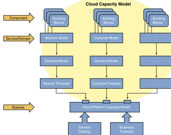
■ It typically will not factor in emerging data center costs such as power consumption. A new capacity-planning process should attempt to provide data that can be used to deliver more business value to the provider and optimize the existing infrastructure and growth. Figure 12-2 illustrates the component parts of the cloud platform forecast model

Cloud Capacity Model Component Service/Domain Busines Compute Model Demand Model Service Catalog Business Forecast Building BlocksBuilding BlocksBuilding Blocks … … Building BlocksBuilding Blocks Building Blocks … Network Model Demand Model Nework Forecast Building BlocksBuilding BlocksBuilding Blocks Compute Forecast

Cloud Platform Capacity Model

Figure 12-2 Cloud Platform Forecast

that define a model for all the component parts and then factor in demand and forecasts for all silos before aggregating this for the cloud platform model.

The following sections will focus on the demand and forecast models, so let’s look at the capacity models. ITIL V3 focuses on capacity in three planes:

■ Business

■ Service

■ Components

Chapter 10, “Technical Building Blocks of IaaS,” discussed the concept of technical build-ing blocks that are the basic reusable blocks that make up a service. From a capacity-planning perspective, we will consider these as components in the overall capacity plan and we will typically group them by technology services or domains within the cloud

platform. Each technology service will have its own demand and forecast model applied to it, as the services will be consumed at different rates. Typically, the storage domain will grow exponentially, whereas compute and networking will fluctuate.

Business capacity is slightly harder to map, so you can refer to this as the cloud platform view, (that is, the capability for the cloud platform to support the services available in the service catalogue). It’s important to view cloud capacity from a tenant services perspec-tive to allow the business to step away from the technology silo view discussed previous-ly and to understand the quantity of services they can deliver.

Network Model

The network model provides a view of the capacity from the perspective of the building blocks that make up the topology-related aspects of the tenant’s service. For example, Chapter 10 introduced the Layer 2 separation building block. In the network model, this will be implemented as a VLAN. From an Ethernet standards perspective, you know that you have a maximum of 4096 VLANs (although this is being addressed with a recently announced Cisco/VMware VXLAN proposal) that can be used in any Layer 2 domain. If you chose to implement a vBlock with Cisco Nexus 7000 acting as the aggregation layer, any Unified Compute System (UCS) that connects to that Nexus 7000 connects to the same Layer 2 domain and so must share this pool of 4096 VLANs.

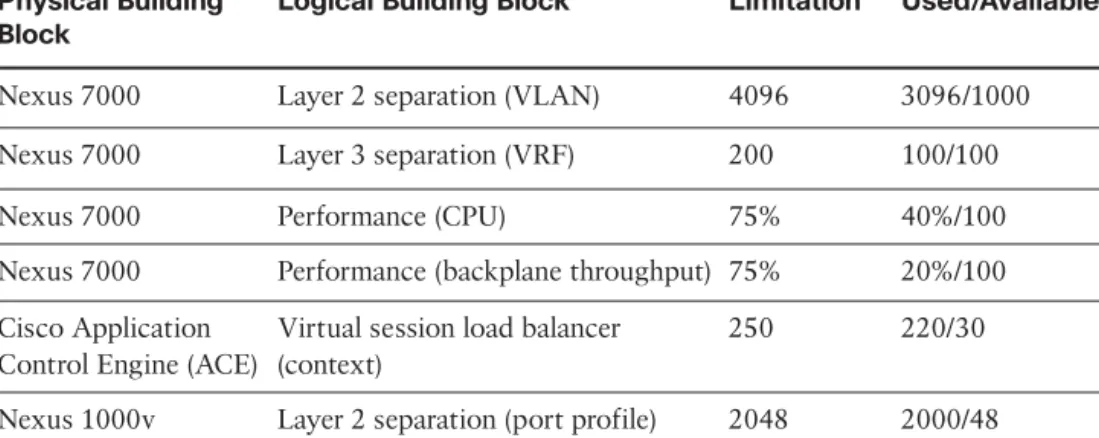
The previous limits can be seen as a capacity limitation from a provisioning point of view; the provisioning systems can only create 4096 VLANs. The performance of the Nexus 7000, CPU and throughput for example, is also a capacity limit, but from the per-spective of service assurance, you can continue to add load to the Nexus until at a cer-tain threshold the performance of all resources will be impacted. We will refer to provi-sioning and capacity limitations as static and dynamic limitations, respectively. The net-work itself is also continuing to be virtualized within the hypervisor with applications such as the Cisco Nexus1000v Distributed Virtual Switch (DVS) and VMware vShield (to name two), which means that the traditional boundary between compute and network is disappearing from a capacity management perspective.1_{Table 12-2 illustrates a capacity} model for some example network building blocks.

Chapter 2, “Cloud Design Patterns and Use Cases,” presented the HTTP/HTTPS load bal-ancer design pattern. To provision and activate a single instance of this pattern that is accessed through the Internet, we would need one VLAN, one port profile, a single load balancer context, and the use of shared Internet Virtual Routing and Forwarding (VRF). Based on a performance baseline, collected by a hypothetical performance management system, you see that each instance will “typically” introduce a 1 percent load on the Nexus 7000 across both the backplane and the CPU (this is just an illustration). This means that the main limiting factor for new service is the load balancer, so only 30 new service instances can be created as the load balancer is shared across multiple tenants. From a bursting perspective, however, given that the two performance building blocks that have been chosen are well within their limits, there should be no issue supporting existing services’ SLAs.

Table 12-2 Example - Network Model Capacity Model

Physical Building Block

Logical Building Block Limitation* Used/Available

Nexus 7000 Layer 2 separation (VLAN) 4096 3096/1000

Nexus 7000 Layer 3 separation (VRF) 200 100/100

Nexus 7000 Performance (CPU) 75% 40%/100

Nexus 7000 Performance (backplane throughput) 75% 20%/100

Cisco Application Control Engine (ACE)

Virtual session load balancer (context)

250 220/30

Nexus 1000v Layer 2 separation (port profile) 2048 2000/48

*Limitation of devices at time of publication; current documentation should be consulted to determine current limitations.

Adding a new Cisco Application Control Engine (ACE) would allow the network domain to support an additional 18 services as this is the next capacity limit (Nexus 1000v). If a new Nexus 1000v was added at the same time, the network domain could potentially support another 250 services (the ACE is the limiting factor). Adding this amount of serv-ices would potentially impact SLAs as the performance thresholds for the Nexus 7000 CPU and backplane could be exceeded, so careful thought must be given to oversub-scription of those two building blocks.

In this example, the ACE and the Nexus 1000V can be considered growth units; more can be added as more services are needed. The Nexus 7000 is not a growth unit; it is the central switch that interconnects all components. When it hits a static of dynamic limita-tion, a new POD would need to be deployed.

Compute Model

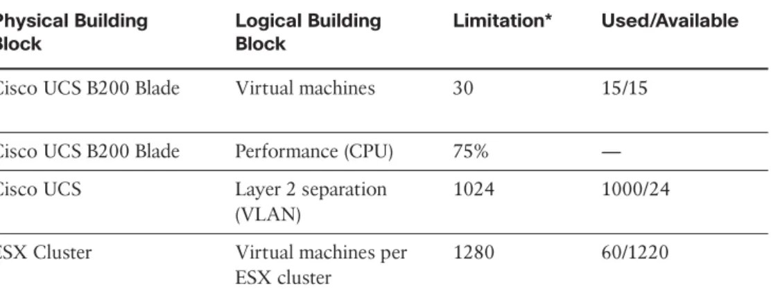
The compute model provides a view of the capacity from the perspective of the building blocks that make up the virtual and physical machines related to the tenant’s service. You will have the same mix of static and dynamic building blocks used for the fulfillment and assurance processes; however, the boundary between these becomes less clear in this domain. For example, although you can say that, as a rule of thumb, a UCS B200 blade should support 30 virtual machines, it of course depends on the resources that those vir-tual machines consume that will make the difference. Thirty virvir-tual machines implement-ing database servers will be different than 30 virtual desktops. As you begin to factor in control plane mechanisms, such as VMware Distributed Resource Scheduler (DRS), which can balance workloads within an ESX cluster based on load, the complexity of managing some of the values outlined in Table 12-3 becomes apparent. Table 12-3 illustrates a capacity model for some example compute building blocks.

Table 12-3 Example - Compute Model Capacity Model Physical Building Block Logical Building Block Limitation* Used/Available

Cisco UCS B200 Blade Virtual machines 30 15/15

Cisco UCS B200 Blade Performance (CPU) 75% —

Cisco UCS Layer 2 separation

(VLAN)

1024 1000/24

ESX Cluster Virtual machines per

ESX cluster

1280 60/1220

*Limitation of devices at time of publication; current documentation should be consulted to determine current limitations.

Rather than focus on all these attributes, consider the Layer 2 separation building block. Cisco UCS extends the VLAN into the compute chassis, but currently supports only 1024 VLANs. After you factor in internal VLANs and any used for storage VSANs, you probably have 900 workable VLANs that can be used in ESX port groups. The previous examples stated that the network topology could support an additional 30 services; how-ever, you can see that, in fact, you can only support an additional 24 services, because this is the limit that the UCS system will support, unless another UCS system is added. Adding another UCS system is not the solution here, unless it connects to a separate Layer 2 domain. In which case, the VLANs can be reused, but you cannot share services at Layer 2 because the VLANs will conflict. The same service running on both UCS sys-tems, in this case, must be interconnected at the IP subnet level. You can see that there is a complex relationship between some of the compute and network models, and this is managed in the cloud platform capacity model.

Storage Model

The storage model provides a view of the capacity from the perspective of the building blocks that make up the storage-related aspects of the tenant’s service. Storage building blocks can be complex to manage, because they might present different views depend-ing on which element you look at. For example, viewdepend-ing a Fibre Channel logical unit (LUN) that has been provisioned with “thin” provisioning from the ESX server perspec-tive will show a different level of consumption than looking at the same LUN from the storage array perspective. So, it’s important to understand what element will provide the most accurate view. Table12-4 illustrates a capacity model for some example storage building blocks.

Table 12-4 Example - Storage Model Capacity Model Physical Building Block Logical Building Block Limitation* Used/Available EMC CLARiiON storage array LUN (FC) 16384 300/16084 EMC CLARiiON storage array LUN performance (IOPS) 20 ms — EMC CLARiiON storage array Gold LUN 16384 100/16084 EMC CLARiiON storage array Gold LUN .vmdk 15 14/1

*Limitation of devices at time of publication, current documentation should be consulted to determine any current

limitations.

Focusing again on the HTTP/HTTPS load balancer design pattern described in Chapter 2, you can assume that the web server virtual machines could require a Gold LUN to store the operating system virtual disks and a Silver LUN for the data virtual disk. You can see that a single Gold LUN has a limit imposed on it of 15 virtual disks per Gold LUN to pre-serve I/O requirements. Fortunately, the CLARiiON will support a large amount of LUNs (depending on sizing), so the storage should not be a limiting factor. However, unless stor-age is reclaimed, the need for new storstor-age continues to grow exponentially and therefore can be a considerable factor later in the cloud platform’s lifetime.

Data Center Facilities Model

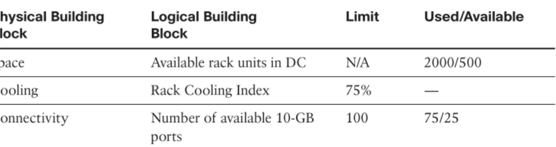
The facilities model provides a view of the capacity from the perspective of the building blocks that make up the physical facilities that support the physical data center equip-ment and tenant services. Traditionally, the capacity of the data center facility, in terms of the consumption and generation of power, heating, cooling, and so on, is modeled at the rack level and aggregated up into a room view and then the data center itself; however, in recent years, the “green” data center view has started to look at the total input/output of the data center. Table 12-5 illustrates a capacity model for some example facilities build-ing blocks.

Table 12-5 Example - Facilities Model Capacity Model Physical Building Block Logical Building Block Limit Used/Available

Space Available rack units in DC N/A 2000/500

Cooling Rack Cooling Index 75% —

Connectivity Number of available 10-GB

ports

100 75/25

The Data Center Maturity Model proposed by Green Grid (www.thegreengrid.org/en/ Global/Content/white-papers/DataCenterMaturityModel)2_{proposes some dynamic} building blocks for general green IT. The Rack Cooling Index (RCI), for example, is a numerical value for air inlet temperature consistency and can be high or low (if applica-ble). For example, if every server is receiving air at the desired temperature, the result is an RCI of 100 percent. If half of the servers receive inlet air that is above the desired tem-perature, the RCI (high) is 50 percent. A Level 2 maturity suggests an RCI of 75 percent across all racks, which in turn drives the physical placement of servers, their efficiency, and the overall design of the cooling system. Making capacity-planning decisions with-out understanding the RCI metric desired will inversely impact the overall efficiency of the data center and that value/cost balance discussed previously. Placing workloads on a physical server will increase the load and therefore the heat output and the cooling required, so again we see a complex relationship between compute and facilities capacity.

Cloud Platform Capacity Model

The Cloud Platform Capacity model provides a holistic view of the capacity and demand forecast across the entire platform. Using the demand forecasts from the “business” for cloud service adoption and the service catalogue as primary inputs, it will aggregate the data from all domains that are considered part of the cloud platform and identify where capacity issues exist, which is easy to say but not easy to implement. It’s fair to say that today, this type of complex capacity management is only available to those with large budgets and resources available to them; however, like all technology issues, time will simplify the solution and provide a more cost-effective solution. So, the principles out-lined in this chapter should be viewed as guidance rather than explicit recommendations. Tools such as VMware Capacity IQ or EMC Unified Infrastructure Manager can provide domain views, whereas tools from performance management companies like Infovista or Netuitive3_{can give a broader “cloud platform” view.}

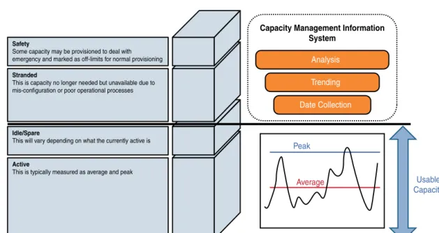
Safety

Some capacity may be provisioned to deal with emergency and marked as off-limits for normal provisioning

Idle/Spare

This will vary depending on what the currently active is

Stranded

This is capacity no longer needed but unavailable due to mis-configuration or poor operational processes

Active

This is typically measured as average and peak

Capacity Management Information System Analysis Trending Date Collection Peak Usable Capacity Average

Figure 12-3 Demand- and Forecast-Based Capacity Management

Demand Forecasting

Demand forecasting is the activity of estimating the quantity of IT services that con-sumers will purchase or use. This data is then used to ensure that capacity can be met both in the short and long term. Demand forecasting typically involves quantitative tech-niques and methods such as trending to determine future demand. Trends describe capac-ity activcapac-ity that has taken place in the past through to the present. A trend might show that demand is increasing, decreasing, or remaining the same. One of the biggest chal-lenges in the cloud is that because of the on-demand nature of cloud requests, demand can be viewed as totally nondeterministic, that is, it is driven by a consumer’s needs, which in a public cloud at least has no relationship to other consumers’ demands. What is seen as a trend one month might simply be a never-repeated pattern. This means that additional analysis is required on top of the trending data to understand the actual pat-terns of cloud usage and to demand management.

Demand forecasting looks at capacity from two perspectives, managing in-flight peak capacity and expected demand. In-flight capacity can be viewed as the usable capacity of a domain, which is comprised of active and idle/spare capacity. Active capacity can be viewed as the average usage of a domain, the average bandwidth consumed through a Nexus 7000, the average CPU of an ESX host, and so on. Idle/spare capacity is the remaining capacity that hasn’t been stranded or allocated as safety buffer; Figure 12-3 illustrates these concepts.

Good operational and capacity management procedures should remove the need for a safety buffer and also highlight and reclaim any stranded resources. However, in reality, these types of capacity limits can take up a large proportion of the usable capacity, and many platform owners today simply “live with it.” From a cloud provider’s perspective, this is simply too high a cost to bear and will really impact the optimization. From an ITIL perspective, all this data is stored and managed in the Capacity Management Information System (CMIS), which acts as the system of record for all resource details. The CMIS can be comprised of many different systems, and in this case, the data in these systems will be federated to provide the capacity manager with a holistic view of all the data relating to capacity of the cloud.

Capacity management can be looked at from a proactive and reactive perspective. The goal of proactive in-flight capacity management is really to ensure that peak demands can always be met without compromising SLAs and maximizing the usable capacity, therefore minimizing spare and stranded capacity. Meeting the peak demand is done by looking at the trends, extrapolating the average peak, and forecasting what the future peak “might” be. Determining the average peak is relatively simple and really just part of statistical analysis. As long as you have enough usable capacity to support the average peak or your SLAs can cope with oversubscribed capacity, this might be the only metric you need. If you take a look at how VMware CapacityIQ4_{calculates the amount of remaining virtual} machines for a given cluster, you can see an example of how this statistical baseline can be implemented. CapacityIQ calculates the remaining virtual machine capacity by using the remaining physical capacity divided by the average virtual machine demand for CPU and average memory consumed:

Remaining VM CPU = Remaining CPU Capacity / CPU Demand for Average VM Remaining VM Memory = Remaining Memory Capacity / Memory Consumed for Average VM

Whichever of these two values is smaller determines how many more virtual machines can be deployed. For example, consider the following scenario for a cluster. An ESX clus-ter has the following:

■ Idle/spare (remaining) CPU capacity of 6 GHz.

■ Idle/spare (remaining) memory capacity is 9 GB.

■ The average virtual machine has 1.5 GHz CPU demand and 4 GB memory consumed. We can make the assumption that these values represent the average new virtual ma-chine’s configuration that will be deployed in this cluster.

If two virtual machines exist in the cluster, there is enough CPU capacity for four virtual machines, but only enough memory capacity to support two virtual machines. The prob-lem with this view is that, although it does provide some level of forecasting, it will be far more accurate where the demand is consistent and less so when demand is variable (that is, driven by a self-service model). CapacityIQ attempts to address this problem by aggre-gating data into what VMware call rollups. A rollupis an average value across a time period. A daily rollup is a number representing the average of the averages for a particular

day. A weekly rollup represents the average across all seven days in the week. CapacityIQ provides rollups based on daily, weekly, monthly, quarterly, and yearly time periods. An alternative approach is to start applying more advanced models such as predictive analy-sis. An example of this is Netuitive, which builds on performance data and adds what it calls a behavioral learning engine to provide the context and trends to this raw data. Unfortunately, neither of these solutions will help the provider if a sudden demand spike means that it runs out of available physical capacity (even if it has safety capacity). Providers should expect this to occur and streamline their procurement process to ensure that these issues are handled as quickly and efficiently as possible.

Expected demand is typically a more qualitative measure coming from a product devel-opment group in telecommunications companies or from a business relationship manager in an ITIL-aligned IT department. Expected demand is a view of what is believed to be the uptake of a service prior to or after it is made available in the service catalogue. This data can be factored into the overall demand forecast, but care should be taken to ensure that the values provided are accurate as they can skew the overall capacity requirements. From a reactive point of view, the provider now has a capacity issue. The proactive capacity management processes have, to some extent, failed, and now the provider is in danger of breaching its SLAs and impacting new requests. If the provider has spare resources such as some safety capacity, this can be used to provide a short-term respite to the problem, but if there is no additional capacity, some workloads must be prioritized over other workloads to ensure that some customers’ SLAs are still met. For example, if tenant 1 has a high SLA or service grade, its workloads need to be prioritized over ten-ants that have a lower SLA or service grade when there is contention and no available spare capacity. This prioritization exercise can occur automatically. For example, in a VMware environment, resource pools can be used to manage resources within a cluster, physical host, or at the VM level, and prioritization is done by the Vsphere control plane without external intervention. For other resources, such as storage- or network-based components, some manual intervention will be required. Clearly, reactive capacity man-agement will have an impact, so when possible, reactive manman-agement should be the exception and not the norm.

Procurement in the Cloud

The capacity model has identified that additional fixed capacity is required, and this means that, for example, additional compute blades are required. This will typically require capital expenditure, which in turn will require the procurement process to adjust fixed capacity to meet the expected demand. We say typicallybecause many vendors, Cisco included, are looking at different financial models to support a public or private cloud that involves operational expenditure rather than CAPEX; however, for the purpos-es of this section, we will consider only the CAPEX model. Figure 12-4 illustratpurpos-es the general impacts of capacity management. In an ideal world, fixed capacity meets the demand. If the expected demand is set too high, there will be a lot of waste. If the expected demand is set to low, there are peaks of resource requirement that cannot be met, which will impact SLAs and the experience of new customers. If there is zero

Ideal Capacity Demand Time Resour ces Under Provisioned Over Provisioned Capacity Demand Time Resour ces Wasted Capacity Demand Time Resour ces

Cost versus Capacity

Time Capacity Breaching SLA Reactive CAPEX Demand Fixed Capacity Predicted Demand Procurement Time

Figure 12-4 Consequences of Capacity Management

procurement time, that is, the physical resources are in stock and already installed, it is possible to cope with demand seamlessly. However, the reality is that typically the hard-ware can take between three weeks and several months to be procured and be made avail-able for service, in which case, SLAs and new cloud services will be impacted.

The cost-versus-capacity model shown in Figure 12-4 summarizes the main issues with capacity management in a cloud environment:

■ The predicted demand is drawn from the business forecast and trends based on cur-rent usage.

■ If the fixed capacity is built in line with predicted demand, as actual demand exceeds both the predicted demand and the fixed capacity, SLAs will be breached and the provision and activation of new services will be impacted. If the procure-ment time for new equipprocure-ment is too long, this might incur SLA penalties or the loss of tenant contracts.

■ Reactive capacity management is not a good thing as it leads to SLA breaches and poor user experience, and so should it be minimized when possible.

Summary

There is no silver bullet for capacity management in a typical data center, so when cloud services are deployed that require a self-service, real-time, on-demand provisioning approach, it gets harder as the demand model is much more challenging to understand. A number of key aspects need to be considered in implementing capacity management for a cloud solution:

■ Implement strong capacity management processes that consider the entire platform service capacity from a holistic manner but also consider business forecasts.

■ Build domain models that track the key service building blocks and growth units.

■ Build measurement and monitoring systems that are capable of performing predictive analysis to extrapolate complex trends.

■ Consider forecasts from the business, but treat them with reasonable level of doubt.

■ Consider the impacts of poor demand management and the impact on procurement.

References

1_{Nexus 7000 VDC scalability, at www.cisco.com/en/US/prod/collateral/switches/} ps9441/ps9402/ps9512/White_Paper_Tech_Overview_Virtual_Device_Contexts.html. 2_{Data Center Maturity Model, at www.thegreengrid.org/~/media/Tools/}

DataCenterMaturityModelv1_0.ashx?lang=en.

3_{Netuitive, at www.netuitive.com/solutions/capacity-management.html.} 4_{CapacityIQ, at www.vmware.com/products/vcenter-capacityiq/overview.html.}