Received 06 February 2007, revised 24 July 2007
Ó 2008, DESIDOC
Design and Simulation of Blending Function for Landing Phase of a UAV
K. Senthil Kumar, C. Sudhir Reddy, and J. Shanmugam
Madras Institute of Technology (MIT), Anna University, Chennai-600 044 ABSTRACT
This paper aims to achieve the autonomous landing of unmanned air vehicle (UAV). It mainly deals with glide path design, flare path design, design of blending function, and interfacing the glide and flare paths with the blending function. During transition from glide slope to flare path, a UAV will tend to the unstable region. In a manned aircraft, the pilot controls the unstability that occurs during the change of phase from glide slope to flare, but which is impossible in UAV till now. A blending function has been formulated for use in a UAV to overcome this unstability during transition. This simulation is done with the Matlab Simulink and the results are reported.
Keywords:UAV, landing phase, glide slope, flare path, blending function, simulation, unmanned air vehicle
1 . INTRODUCTION
Over the past few decades, a keen interest is growing for the development of flying objects of small size for a variety of civilian and military applications. An unmanned autonomous aerial vehicle can perform tasks which would be exceedingly difficult or hazardous for a manned vehicle. Possible applications of this technology include search, rescue, surveillance, aerial mapping, inspection of structures like bridges and power lines, particularly in environmental conditions where human guided flights are not possible. The strategic importance of their use as reconnaissance aircraft is easily understood. Various attempts have been made to automate the control of an aerial flying vehicle. An unmanned air vehicle (UAV) is expected to complete the mission and return to the base in an autonomous manner. The recovery of a UAV is the most challenging and hazardous part of a UAV's flight.
2 . PROBLEM STATEMENT
In this paper, an attempt has been made to design and simulate the blending function for landing phase of a UAV. The landing phase is divided into two parts, viz; glide path and flare path. The problem faced during the transition from glide path to flare is clearly addressed in this paper. A new concept termed as blending function during the transition region is discussed and a possible solution is suggested. Flying aircraft are subject to wind disturbances1,2
that can be fatal when these occur close to the ground while landing. However, this problem is not addressed in this paper due to autoland systems that are routinely employed are not designed to handle large wind gusts that occasionally occur.
3. DESIGN OF BLENDING FUNCTION The blending function is mixing of signals during the transition from glide path3-8 to flare path 3-7,9.
This function is conceived to solve the problem of extreme oscillations and instability during the transition period. The proposed geometry of blending function is shown in Fig.1. In the blending function, the gain of glide and flare paths is varied according to variation in range. It is observed that the glide path gain is decreasing and the flare path gain is increasing. By using a limiter, the upper limit of the gain is set to 1 and the lower limit is set to 0. At any point the sum of the glide and the flare path gain is 1. From range R1 to R3, the glide path alone will be present, the gain of the glide path is 1 and the flare path gain is 0. From R2 to 0 only the flare path will be present, the glide path gain is 0 and the flare path gain is 1. In between R3 and R2 the blending function will occur and the gain will vary with glide path gain decreasing from 1 to 0 and flare path gain increasing from 0 to 1. The conditon of the range is ( R1> R3> R2> 0). Here, R1 is the point from which glide path starts; Gg1 is the gain at which glide path starts; R2 is the range at which glide path gain becomes zero; R3 is the range at which flare path gain becomes zero; and Gf1 is the flare path gain at R1.
The equation of straight line with coordinates (x1, y1) and (x2, y2) is given by 2 1 1 1 2 1
(
y y
)
y
y
(
x x
)
x
x
--
=
--
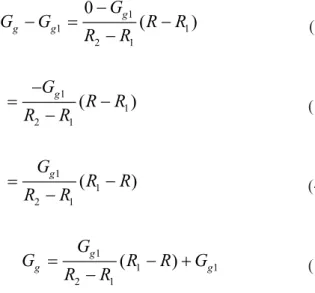
(1) such that the glide path gain equation with the coordinates (R1,Gg1) and (R2,0) as 1 1 1 2 10
(
)
g g gG
G
G
R R
R
R
--
=
--
(2) 1 1 2 1(
)
gG
R R
R
R
-=
--
(3) 1 1 2 1(
)
gG
R R
R
R
=
--
(4) 1 1 1 2 1(
)
g g gG
G
R R G
R
R
=
-
+
-
(5) where Gg is the Glide path gain at every instant of range R, and the flare path gain equation with the coordinates (R1, Gf1) and (R3, 0) as 1 1 3 3 10
(
)
f f fG
G
G
R R
R
R
+
-
=
--
(6) 1 3 3 1(
)
fG
R
R
R
R
=
--
(7) 1 3 1 3 1(
)
f f fG
G
R
R
G
R
R
=
-
+
-
(8) where Gf is the flare path gain at every instant ofrange R.
In the region between range R3 and R2 the blending phenomenon will occur.
4. MATLAB IMPLEMENTATION OF BLENDING FUNCTION Here R2=3000; R3=5000; G = 3 2 1 R R
-The geometrical implementation of the blending equations using Matlab Simulink11-13 is shown in
Fig. 2 and the interfacing of blending function with the glide and flare paths is shown in Fig. 3.
5 . RANGE AND HEIGHT CALCULATION Figure 4 illustrates the geometry to find out the instantaneous range of UAV which mainly depends upon the latitude, longitude and altitude (LLA) of the UAV and the destination runway.
The latitude conversion to feet is relatively constant from the equator to the poles and is approximated at all points as 6076 ft/min. The longitude conversion to feet varies from the equator to the poles. This is because the lines of longitude become closer towards the poles. The circle created by intersecting a plane with the earth at some line of latitude will have a radius equal to the radius of the earth times the cosine of the latitude angle. The radius of this circle is used to calculate the circumference of the earth at that particular latitude. Regardless of the circumference of the circle, it still contains 3600,
thus a conversion factor can be calculated. The website www.earth.google.com14 provides
commonly used constants, conversion factors and measurements. Google earth provides the average
radius of the earth as 36,522 ft. This then yields the conversion factor for longitude as 36,522*cos(latitudeo) ft/min.
The steps involved for LLA calculation are: (i) known parameteres are airport latitude, airport longitude, base elevation of the runway and initial ground distance from which glide path starts,
(ii) based on range, height of aircraft above base elevation are calculated, and
(iii) the aircraft LLA is calculated as:
ini head 1 initial Threshold
Gd cos( T ) Lat = lat
180 6076 60 p ´ ´ ´ + ´ (9) ina head initial Threshold Initial 1 Gd sin( T ) 180 6076 60 Lon = lon cos( lat ) 180 p ´ ´ ´ ´ + p ´ (10) Threshold
Base elevation = alt (11)
Figure 2. Blending function.
Initial Initial
alt = h +Base elevation (12) (iv) the runway end LLA is calculated as
ina head Initial Runwayend [{Gd +Runway length} ð 1 ×cos( ×T )× ]+lat 180 6076×60 =lat é ù ê ú ê ú ê ú ë û (13) ina head Initial Initial Runwayend ð 1 [Gd +Runway length}×sin( ×T )× ] 180 6076×60 lon ð cos( × lat ) 180 = lon é ù ê ú + ê ú ê ú ë û(14) Runwayend
Base elevation= alt (15) (v) instantaneous range and height is calculated
as:
[
]
2 Threshold Initial 2 Threshold Initial Initial 2 Threshold Initial initial [ lat - lat ] 6076 60 [ lon - lon ] 6076 60 cos( lat 180 [ alt - alt ] range ´ ´ + ´ ´ ´ é ù ê p ú ê ´ ú ê ú ë û + = (16)[
]
2 Ins Initial 2 Ins Initial Initial 2 Ins Initial Delta [ lat - lat ] 6076 60 [ lon - lon ] 6076 60 cos( lat ) 180 [alt - alt ] g ran e ´ ´ + ´ ´ ´ é ù ê p ú + ê ´ ú ê ú ë û = (17)Initial Delta Ins
range range- = range (18)
Ins Ins
alt Base elevation = h- (19) The symbol and description of the various parameters used in the equations are given below:
Figure 4. Latitute, longitude, and altitude calculations.
Symbol Description Symbol Description
Gdini Initial ground distance Thead True heading
Latinitial Initial latitude loninitial Initial longitude
altinitial Initial altitude latThreshhold Threshold latitude
lonthreshhold Threshold longitude altThreshhold Threshold altitude
latrunwayend Runwayend latitude lonRunwayend Runwayend longitude
altrunwayend Runwayend altitude rangeinitial Initial Range
RangeDelta Change in range rangeins Instantaneous height
5.1 Sample Calculation
In this paper, the Dallas Fort Worth International Airport has been considered for the landing phase of UAV with the following known parameters: True heading of 180.3 deg, base elevation of 607 ft, latitude of 2.93483568652165 deg, longitude of 97.0268825156042 deg and Initial ground distance of 24300 ft. These values are used to calculate initial range, instantaneous range, initial height and instantaneous height. Using steps (iii) to (v), the calculated values are:
Initial height = 1060.960 ft Initial altitude = 1667.96 ft
Initial latitude = 33.00149046735776° Initial longitude = 97.0272315271941°
Runway-end altitude = base elevation = 607 ft Runway length = 6076 ft Runway-end latitude = 32.91816924831753° Runway-end longitude = 97.0267952483441° Initial range = 24323.1502096 ft Delta range = 6361 ft Instantaneous range = 24323.15020966361=17962 ft With simulation run in Matlab Simulink environment for about 20 s, it is observed that the simulated instantaneous range is equal to the calculated instantaneous range. Hence, it has been proved that the algorithm is more efficient and this has been verified with many more airports around the world.
6. SIMULATION RESULTS 6.1 Gain Variation with Range
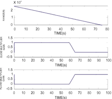
The simulation input namely latitude, longitude and altitude are given from the airport selector function and these values are used to calculate the range. The simulation results are shown in Figs 58. In Fig. 5, the range, glide multiplier gain and flare multiplier gain variation with time is shown. At the glide starting point, the range is around 23,000 ft
and by the time it reaches 86 s, the range is 0 ft. This implies that landing has been accomplished. Table 1 describes the gain variation with range starting from glide slope to touch down point.
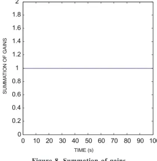
Figure 6 shows the variation of the glide multiplier gain with range and it is observed that from glide slope starting point, i.e., 23,000 ft to 5000 ft, the gain remains as 1 between 5000 ft and 3000 ft, the gain gradually decreases from 1 to 0 and from 3000 ft to touch-down point, the gain decreases to 0. Figure 7 shows that the flare multiplier gain varies from 0 to 1. The flare starting point is 5000 ft and up to that point, the gain is 0, and from 3000 ft to touch-down point the gain remains as 1. It means that in the flare path between 5000 ft and 3000 ft, the gain is increasing from 0 to 1. It is observed from Figs 6 and 7 that between 5000 ft and 3000 ft, the glide path gain is decreasing, the flare path gain is increasing, and the blending phenomenon is said to occur. From Fig. 8, it is inferred that the summation of the glide and flare path gain always remains as 1.
Range (ft) Glide path gain Flare path gain
23000-5000 1 0
5000-3000 1à 0 0 à 1
3000-0 0 1
Table 1. Gain variation with range
Figure 5. Response of range, glide multiplier gain, and flare multiplier gain.
6.2 Response of the Parameters Variation without Blending Function
The responses of the various parameters without using blending function are shown in Figs 9-15.The flare path starts at 3000 ft, above 3000 ft glide path alone will be present. In terms of time, upto 65 s only glide path will be present and after 65 s the flare path alone will be present.
From Fig.15 it can be observed that during transition from glide slope to flare path, the UAV will experience large variation warranting more deflection in the elevator command which is not recommended during this transition.
6.3. Responses of the Parameters Variation with Blending Function
The responses of the various parameters with the blending function are shown from Figs 1622. The blending phenomenon occurs from 5000 ft to 3000 ft, which means that between 5000 ft and 3000 ft the UAV will be in both glide path and flare path. Above the altitude of 5000 ft (i.e., from 23000 ft to 5000 ft) the UAV will be
0 10 20 30 40 50 60 70 80 90 100 0 0.2 0.4 0.6 0.8 1 1.2 1.4 1.6 1.8 2 TIME (s) SU M M AT IO N OF GAINS
Figure 8. Summation of gains. Figure 6. Glide multiplier gain versus range.
RANGE (ft)
GLIDE MUL
TIPLIER GAIN
Figure 7. Flare multiplier gain versus range.
RANGE (ft) GLIDE MUL TIPLIER GAIN 0 10 20 30 40 50 60 70 80 90 100 -5 0 5 10 TIME (s) A N GLE OF A TT A C K (deg) 0 10 20 30 40 50 60 70 80 90 100 -5 0 5 10 x 10 -3 S ID E S LIP (deg) TIME (s)
in the glide path and below the altitude of 3000 ft (i.e., from 3000 ft to touch-down point), it will be in the flare path only. In terms of time, the blending phenomenon will occur between 59 s and 65 s. During 059 s, only the glide path will be present and after 65 s, only the flare path will be present.
7 . COMPARISON OF PERFORMANCE WITH AND WITHOUT BLENDING FUNCTION
The Figs 2330 show the comparison of angle of attack, sideslip, height, pitch rate, roll rate, and yaw rate with and without blending function. The dotted lines indicate the parameter variation with blending function and thick lines indicate the parameter variation without blending function. The parameters are compared with range variation.
From 5000 ft to 3000 ft with time variation from 59 s to 65 s, the angle of attack variation with
HE IG HT (ft) DE CE NT R A TE (f t/s ) 0 10 20 30 40 50 60 70 80 90 100 -500 0 500 1000 1500 TIME (s) 0 10 20 30 40 50 60 70 80 90 100 -30 -20 -10 0 TIME (s)
Figure 10. Responses of height and decent rate.
0 10 20 30 40 50 60 70 80 90 100 -0.50 0.5 x 10⁻¹⁰ TIME(s) R O LL R A TE (deg/ s) 0 10 20 30 40 50 60 70 80 90 100 -20 0 20 TIME(s) PI TC H RAT E (deg/ s) 0 10 20 30 40 50 60 70 80 90 100 -0.50 0.5 x 10⁻¹⁰ TIME(s) YAW RAT E (deg/ s)
Figure 12. Responses of yaw rate, pitch rate, and roll rate.
Figure 13. Responses of aircraft velocity in x, y, and
z directions. 0 200 400 V E LO CI TY IN X D IR E C TI O N (ft/ s) -0.2 0 0.2 0 10 20 30 40 50 60 70 80 90 100 -50 0 50 TIME (s) 0 10 20 30 40 50 60 70 80 90 100 TIME (s) 0 10 20 30 40 50 60 70 80 90 100 TIME (s) V E LO CI TY IN Y D IR EC TI O N (ft/ s) V E LO CI TY IN Z D IRE C TIO N (ft/ s) 0 10 20 30 40 50 60 70 80 90 100 -0.1 0 0.1 TIME (s) R O LL (deg) 0 10 20 30 40 50 60 70 80 90 100 -10 0 10 TIME (s) P ITCH (deg) 0 10 20 30 40 50 60 70 80 90 100 -200 0 200 TIME (s) Y A W (deg)
0 10 20 30 40 50 60 70 80 90 100 -180 -160 -140 -120 -100 -80 -60 -40 -20 0 20 TIME (s) ELE V ATO R COMM A N D (d eg )
Figure 15. Response of elevator command.
-500 0 500 u ai r (f t/s ) -0.2 0 0.2 0 10 20 30 40 50 60 70 80 90 100 -50 0 50 TIME (s) 0 10 20 30 40 50 60 70 80 90 100 TIME (s) 0 10 20 30 40 50 60 70 80 90 100 TIME (s) v a ir ( ft/ s) w ai r (f t/s )
Figure 14. Responses of air velocities in x, y and z
directions.
Figure 16. Responses of angle of attack and side slip. -5 0 5 10 AN G LE O F AT TAC K (d eg ) 0 10 20 30 40 50 60 70 80 90 100 -0.01 0 0.01 0.02 0.03 TIME (s) S ID E S LI P(deg) 0 10 20 30 40 50 60 70 80 90 100 TIME (s) TIME (s) -500 0 500 1000 1500 HE IG HT (f t) 0 10 20 30 40 50 60 70 80 90 100 -30 -20 -10 0 DE CE N T R A TE (f t/s ) TIME (s) 0 10 20 30 40 50 60 70 80 90 100
Figure 17. Responses of height and decent rate.
-0.1 0 0.1 R O LL (d eg ) -10 0 10 P ITC H (d eg) 0 10 20 30 40 50 60 70 80 90 100 -200 0 200 TIME (s) YAW ( de g) 0 10 20 30 40 50 60 70 80 90 100 0 10 20 30 40 50 60 70 80 90 100
Figure 18. Responses of roll, pitch, and yaw angles.
-5 0 5 x 10 -3 RO LL RA TE (r ad ) -0.5 0 0.5 P IT C H RA TE (r ad ) 0 10 20 30 40 50 60 70 80 90 100 -2 0 2 x 10 -3 TIME (s) YAW R A TE (r ad ) 0 10 20 30 40 50 60 70 80 90 100 0 10 20 30 40 50 60 70 80 90 100
58 59 60 61 62 63 64 65 66 67 5 5.2 5.4 5.6 5.8 6 6.2 6.4 6.6 TIME (s) AN G LE OF AT TAC K (d eg )
WITHOUT BLENDING FUNCTION WITH BLENDING FUNCTION
Figure 23. Response of angle of attack.
0 10 20 30 40 50 60 70 80 90 100 -15 -10 -5 0 5 10 TIME (s) ELEV AT OR C O M M AN D (deg
Figure 22. Response of elevator command.
and without blending function is as shown in Fig. 23. On comparison, it is observed that when the blending function is not included, the variation is large, i.e., around 15 per cent, but when the blending function is included, the variation is reduced to about 3 per cent.
The decent rate shown in Fig. 24 is smoother with the blending function than when compared to without the blending function. The smooth variation of decent rate means that when the oscillations get reduced, the steepness will also get reduced.
The comparison of heights shown in Fig. 25 proves that the steepness of the aircraft is reduced.
The exponential decay is found to be good when including blending function. If the steepness increases, i.e., without blending function, the force on the landing gear will also be increased. This may cause the landing gear failure and wear of tires, which makes the landing of the aircraft difficult.
On comparing the pitch rate as shown in Fig. 26, it is observed that the variation and the oscillations are considerably more when the blending function is not included. The variations are reduced when the blending function is included.
The comparison of pitch is shown in Fig. 27. It is observed that the instant pitch is available by
-200 0 200 400 VE LO C ITY IN X DI R E CT IO N ( ft/ s) -0.1 0 0.1 0 10 20 30 40 50 60 70 80 90 100 -50 0 50 TIME (s) 0 10 20 30 40 50 60 70 80 90 100 0 10 20 30 40 50 60 70 80 90 100 VE LO C ITY IN Y DI R ECT IO N (f t/s ) VE LO C ITY IN Z DI R ECT IO N (f t/s )
Figure 20. Responses of aircraft velocites in x, y, and z directions.
0 10 20 30 40 50 60 70 80 90 100 -500 0 500 ua (f t/s ) 0 10 20 30 40 50 60 70 80 90 100 -0.1 0 0.1 0 10 20 30 40 50 60 70 80 90 100 -50 0 50 TIME (s) va (f t/s) wa (f t/s )
58 59 60 61 62 63 64 65 66 67 -20 -18 -16 -14 -12 -10 -8 -6 -4 -2 0 TIME (s) DE CE NT R A TE (f t/s )
WITH BLENDING FUNCTI ON WITHOUT BLENDING FUN CTION
Figure 24. Response of decent rate.
58 59 60 61 62 63 64 65 66 67 0 50 100 150 200 250 300 TIME (s) HEIGHT (ft)
WITH BLENDING FUNCTION WITHOUT BLENDING FUNCTION
Figure 25. Response of height.
58 59 60 61 62 63 64 65 66 67 -2.5 -2 -1.5 -1 -0.5 0 0.5 1 1.5 2 TIME (s) PI TC H RATE (de g/s )
WITHOUT BLENDING FUNCTION WITH BLENDING FUNCTION
Figure 26. Response of pitch rate.
58 59 60 61 62 63 64 65 66 67 2 2.2 2.4 2.6 2.8 3 3.2 3.4 3.6 TIME (s) PI TCH (d eg )
WITHOUT BLENDING FUNCTION WITH BLENDING FUNCTION
58 59 60 61 62 63 64 65 66 67 300 305 310 315 320 325 330 335 340 345 350 TIME (s) VE LO C IT Y IN x D IR E C TIO N ( ft/
s) WITH BLENDING FUNCTIONWITHOUT BLENDING FUNCTION Figure 27. Response of pitch.
Figure 28. Response of velocity in x-direction.
58 59 60 61 62 63 64 65 66 67 25 30 35 40 TIME (s) VE LO C IT Y IN z D IR E C TIO N ( ft/ s)
WITH BLENDING FUNCTION WITHOUT BLENDING FUNCTION
58 59 60 61 62 63 64 65 66 67 -180 -160 -140 -120 -100 -80 -60 -40 -20 0 20 TIME (s) E LE V A TOR COM M A N D (deg)
WITHOUT BLENDING FUNCTION WITH BLENDING FUNCTION
Figure 30. Response of elevator command.
summing the pitch at the previous instant and the pitch rate at that instant. Hence, when the pitch rate varies, the pitch will also vary automatically.
The variation of velocities wrt x- and z-directions are shown in Fig. 28 and Fig. 29 respectively with and without the blending function. The blending function ensures reduced velocity in z -direction which will cause smooth contact of the wheels with surface on touch down.
The elevator command, which is given to the elevator, is shown in Fig. 30, with and without blending function. The elevator deflection seems to be more when the blending function is not used, requiring more control power which might cause damage to control surface, resulting in fatal accidents during landing. Using the blending function, the control power required to move the elevator is substantially reduced.
Thus, using blending function, the oscillations are reduced and the control power is also considerably reduced as evident from the graph and ensures safe landing.
Parameter Without blending function With blending function
Angle of attack Variation is high Variation is low
Decent rate Sudden change Smooth change
Height Steepness is high Steepness is low
Pitch rate Variation is high Variation is low
Pitch Variation is high Variation is low
Forward velocity in x-direction Variation is not smooth Variation is smooth Forward velocity in z-direction Variation is high Variation is low
Elevator command High deflection Small deflection
Table 2. Performance measures
Parameters At the glide slope begin (0 s) At the start of blending function (59 s) At the end of blending function (65 s) At touch-down point (86 s)
Angle of attack (deg) 2 6 5.6 - 0.3
Sinkrate (ft/s) 20.8 14.71 - 18.6 - 0.001
Altitude (ft) 1074 221 123 7.5
Pitch rate (deg/s) 3.7 - 0.014 - 0.5 0
Pitch angle (deg) 0.5 3.5 2.5 - 0.3
Incremental forward velocity (ft/s) 325 330 332 184
Incremental vertical velocity (ft/s) 12 35 32.6 - 1
Throttle 0.045 - 0.06 0.2466 0.1
Elevator command (deg) 0.18 0.2696 - 0.06 0
Range (ft) 24330 5000 3000 0
8 . COMPARISON OF PERFORMANCE MEASURES
Measures of performance6 are required to specify
the desired landing conditions of aircraft. Basically, they require that the aircraft must land within the desired envelope of dispersions. Table 2 summarises the blending performance measures.
9 . CONCLUSIONS
In the present study, a blending function has been formulated for use in an UAV using simulation with Matlab Simulink. From the simulation results, it is inferred that the blending of signals during transition from glide slope to flare solves the problem of unstability and extreme oscillations. The property of the blending function has proved that the summation of the gains is always equal to 1. It is evident that the landing of the UAV using blending function gives good performance measures.
ACKNOWLEDGMENTS
The authors would like to express their sincere thanks and gratitude to Dr P.A. Janaki Raman, Professor, Dept of Electrical Engineering, Indian Institute of Technology Madras, Chennai; Shri P.S. Krishnan, Director Aeronautical Develop-ment EstablishDevelop-ment, Bangalore; and Shri K.V. Srinivasan, Scientist G, ADE, Bangalore, for their inspiration and encouragement for successful completion of this work.
REFERENCES
1. Ih-Gau, Juang & Jern-Zuin, Chio. Fuzzy modeling control for aircraft automatic landing system.
Int. J. Syst. Sci., 2005, 36(2), 77-87.
2. Neuman, F. & Foster, J.D. Investigation of a digital automatic aircraft landing system in turbulence. NASA Ames Research Center, Moffet Field, CA.,1970, NASA-TND-6066.
3. Yong,Tao. & Yongzhang, Shen. Guidance and control for automatic landing of UAV. Trans. Nanjing Univ. Aero. Astro., 2001, 18(2), 229-35.
4. Blakelock, J.H. Automatic control of aircraft and missiles. John Wiley Sons, NY., 1990. 5. McLean, Donald. Automatic flight control systems.
Prentice-Hall Publications, 1990.
6. Senthil Kumar, K.; Shanmugam, J. & Srinivasan, K.V. Neural network approach for autopilot and landing phase of unmanned air vehicle. In
1st Indian International Conference on Artificial
Intelligence, 2003. pp. 1028-037
7. Li,Y.; Sundararajan, N.; Saratchandran, P. & Wang, Z. Robust neuro-H8, controller design for aircraft auto-landing. IEEE Trans. Aero. Elec. Syst., 2004, 40(1), 158-67.
8. Senthil Kumar, K.; Reddy, Sudhir C. & Shanmugam, J. Design of glide slope control system for landing phase of large unmanned aerial vehicle. In Proceedings of the International Conference on High Speed Transatmospheric Air and Space Transportation, 29-30 June 2007, Hyderabad, Aeronautical & Astronautical Societies of India, pp. 99-108 9. Charles, C.; Jorgensen & Schley, C. A neural
network baseline problem for control of aircraft flare and touch-down, edited by W. Thomas Miller lll; Richard S. Sutton and Paul J. Werbos. pp. 403-25.
10. Pasko, G.; Pasko, A. & Kunii, T. Bounded blending for function-based shape modelling, Pre-final version before editing by the IEEE CG&A. pp. 36-45.
11 MAT LAB User's Manual User's Guide. The Math Works Inc, 2004.
12. Simulink User's Manual User's Guide. The Math Works Inc, 2004.
13. Control System Toolbox User's Manual. The Math Works Inc, 2004.