Inside debt renegotiation: Optimal debt reduction,
timing, and the number of rounds
Franck Moraux, Florina Silaghi
To cite this version:
Franck Moraux, Florina Silaghi. Inside debt renegotiation: Optimal debt reduction, timing,
and the number of rounds. Journal of Corporate Finance, Elsevier, 2014, 2014 (27), pp.269-295.
<
10.1016/j.jcorpfin.2014.05.012
>
.
<
halshs-01024229
>
HAL Id: halshs-01024229
https://halshs.archives-ouvertes.fr/halshs-01024229
Submitted on 12 Oct 2014
HAL
is a multi-disciplinary open access
archive for the deposit and dissemination of
sci-entific research documents, whether they are
pub-lished or not.
The documents may come from
teaching and research institutions in France or
abroad, or from public or private research centers.
L’archive ouverte pluridisciplinaire
HAL, est
destin´
ee au d´
epˆ
ot et `
a la diffusion de documents
scientifiques de niveau recherche, publi´
es ou non,
´
emanant des ´
etablissements d’enseignement et de
recherche fran¸cais ou ´
etrangers, des laboratoires
publics ou priv´
es.
Inside debt renegotiation: Optimal debt reduction, timing, and the number of
rounds
Franck Morauxa, Florina Silaghia,∗
aUniversit´e de Rennes 1, 11, Rue Jean Mac´e, 35000, Rennes, France
Abstract
This paper develops a model of debt renegotiation in a structural framework that accounts for taxes, bankruptcy costs and renegotiation costs. To our knowledge, all the previous work on debt renegotiation implies an infinite number of renegotiations. This feature preempts the analysis of the optimal number of renegotiations. We address this drawback by incorporating fixed renegotiation costs in a model of multiple renegotiations, hence obtaining a small finite number of renegotiations. Simple analytical formulae are derived for debt and equity, as well as implicit formulae for the coupon reduction, as a result of a backward recursive technique. The results show that the optimal number of renegotiations, the size and the dynamics of the coupon reductions depend critically on the bargaining power of the claimants. Testable empirical implications regarding multiple costly renegotiations are drawn.
Keywords: Debt renegotiation, Debt pricing, Strategic contingent claim analysis
JEL:G30, G32, G33, G13
∗Corresponding author. Tel.:+33 (0)2 23 23 78 08; fax:+33 (0)2 23 23 78 34.
Email addresses:[email protected](Franck Moraux),[email protected](Florina Silaghi)
*Manuscript
“The basic idea was to make debt relief acceptable to commercial bank creditors by offering a smaller but much safer payment stream in exchange for the original claim that clearly could not be serviced in full.”,Sturzenegger and Zettelmeyer(2007)1
1. Introduction
Although there exists an abundant literature on debt renegotiation, to our knowledge, all previous work implies an infinite number of renegotiations. This feature preempts the analysis of the optimal number of renegotiations. In this paper, we address this drawback by incorporating fixed renegotiation costs in a model of multiple renegotiations, hence obtaining a small finite number of renegotiations.
Debt renegotiation is important and quite common, both at corporate and sovereign level. It exists in formal legal contexts and in private workouts.2,3 It also appears in very closely related situations such as breach of covenants,4
LBO restructuring and corporate bond clawbacks.5
Preliminary thoughts on debt renegotiation are offered byLeland(1994) in the eighth section of his famous article. A rigorous analysis of debt renegotiation is then presented in strategic debt service models (SDS hereafter), as in the papers ofAnderson and Sundaresan(1996),Mella-Barral and Perraudin(1997) andFan and Sundaresan(2000), to name only a few. SDS consists of arbitrary “take-it-or-leave-it” offers (from the equity holder to creditors or from creditors to the equity holder) that result in atemporary reduction in the coupon. Mella-Barral (1999),Hege and Mella-Barral(2000) andLambrecht(2001) on the other hand, model debt renegotiation in the form ofpermanent
coupon reductions.6
In a SDS setting, the firm is financed with a perpetual debt whose coupon is paid in full as long as an underlying state variable (assets value or output price) remains above a certain renegotiation threshold. When this threshold is reached from above for the first time, the firm starts paying a lower coupon and retakes the full coupon payment as soon as the firm recovers, i.e. when the state variable reaches the threshold from below. The initial coupon level can be reduced and restored many times with no constraint. This unconstrained view to proceed has been proved to have a clear advantage for finding analytical formulae. But this stylized way has some clear drawbacks too.
First, the number of renegotiations is possibly infinite, which of course is not realistic. Second, we consider that SDS models emphasize effects of temporary missed interest payments rather than effects of the permanent solution debt and equity holders may look for. Third, in some SDS models, the firm can strategically avoid bankruptcy through an infinite number of renegotiations, which is not the case in the real world.
Mella-Barral(1999) proposes a model with permanent coupon reductions in which selling the assets of the firm becomes preferable to continuing operating it. It therefore addresses two of the drawbacks of SDS models. However, in this model each time the state variable reaches a new minimum, the coupon will be reduced by an infinitesimal amount. This continuous way of reducing the coupon implies the firm could potentially have an infinite number of renegotiations in a finite period of time. Hence, this model also suffers from the main drawback of SDS models in the sense that the number of renegotiations is potentially infinite.
1It is worth having a look at the rich economic literature on sovereign debt renegotiation as this issue has been extensively studied compared
to corporate debt renegotiation. The clear-cut description of the Brady plan (a plan for sovereign debt restructuring at the end of the 1980s in Latin America) made bySturzenegger and Zettelmeyer(2007) captures the essence of our model.Suter(1992) reveals that for interwar sovereign defaults, interest payments suffered an average haircut of 34% and face values were reduced by 23%. For recent evidence on sovereign debt renegotiation seeBai and Zhang(2012).
2Empirical studies demonstrate that private workouts are quite often considered by firms in financial distress.Gilson et al.(1990), for instance,
find that about half of the 169 firms they consider resolve distress through private workouts. A very strong incentive is that costs of private workouts are significantly lower than formal bankruptcy costs (see againGilson et al.,1990,Franks and Torous,1989andBris et al.,2006).
3Favara et al.(2012) show that equity risk is smaller in countries in which the bankruptcy code favors formal debt renegotiation. 4SeeGarleanu and Zwiebel(2009) for an analysis of debt covenants renegotiation.
5For recent evidence on corporate bond clawbacks seeDaniels et al.(2013).
6Debt renegotiation may lead however to other kinds of restructuring such as debt equity swaps and maturity extension (seeFan and Sundaresan, 2000andLongstaff,1990respectively). Debt renegotiation with multiple lenders is analyzed byDumitrescu(2007),Hackbarth et al.(2007) and
Hege and Mella-Barral(2005).Chen(2003) andShibata and Tian(2010,2012) study debt renegotiation in the presence of asymmetric information.
In this paper, we follow Mella-Barral(1999) by modeling debt renegotiation in the form of permanent coupon reductions. However, we believe it is important to account for frictions that prevent infinite renegotiations. We thus incorporate a fixed renegotiation cost. This allows us to answer an important question regarding what the optimal number of renegotiations should be. To the best of our knowledge, we are the first to address this question. We present a new continuous time model of debt renegotiation in which we derive and investigate the effects of finite costly renegotiations on equity, debt, firm value, capital structure and the optimal number of renegotiations.
We consider a firm financed by equity and a perpetual debt. Following Leland (1994), the equity holder decides optimally when to stop paying the coupons and defaults at an endogenously determined bankruptcy threshold. At any point in time between debt issuance and bankruptcy time, the party that has all bargaining power can propose renegotiation in the form of a permanently reduced coupon, while keeping the other party indifferent at its reservation value.7 The party with all bargaining power optimally decides the renegotiation thresholds, the coupon reductions and
the optimal number of renegotiations in order to maximize its claim value.
We analyze two polar cases in which either the equity holder or the creditors have all bargaining power. Moreover, we incorporate a parameter that captures the bargaining power of each party. This allows us to derive implications and discuss the solutions of our model for a general distribution of bargaining power.
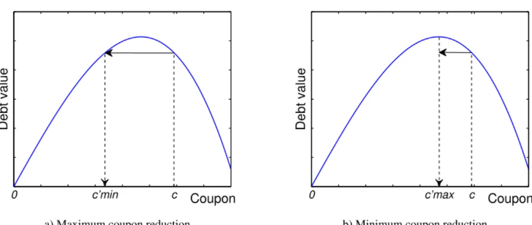
We first present a benchmark model of one single costless renegotiation. When the equity holder has all bargaining power, she proposes renegotiation at Leland’s default threshold, maintaining debt value constant.8 The later the equity holder renegotiates, the higher the coupon reduction she will be able to obtain from creditors. As inLeland(1994), debt value is a hump-shaped function of the coupon, which means there exists a coupon for which debt value is maximized. When the assets value deteriorates, the initial coupon agreed with the creditors is above the coupon that maximizes debt value, which implies that the equity holder is paying a high unsustainable coupon. Reducing the coupon would actually increase debt value (as long as the reduced coupon is above a minimum acceptable coupon that maintains debt value constant).
When creditors have all bargaining power, they also want to renegotiate as late as possible, at the same renegoti-ation threshold. Regarding the coupon reduction, we show that the coupon should be reduced at least to 67% of the initial value, and at most to 27% of the initial coupon level (for our baseline case). Any coupon value above 67% is Pareto dominated, as we could further reduce it and improve both the value of debt and equity. The coupon cannot be reduced beyond 27% as creditors would refuse renegotiation. The exact size of the coupon depends on the bargaining power of claimants. To our knowledge, this is the first paper to provide a range for the optimal coupon reduction. Additionally, we find that renegotiation increases total firm value and that the renegotiation surplus can be shared among claimants according to their bargaining power.
In the general framework that allows for multiple costly renegotiations we obtain a series of new interesting results. When the equity holder has all bargaining power, we have a “cascade” of coupon reductions. Each time the assets value reaches Leland’s default threshold corresponding to the current coupon value, the coupon will be significantly reduced. At each renegotiation stage the firm is downsized in the same proportion. Given the renegotiation costs, the equity holder will only renegotiate a very small number of times.
When creditors have all bargaining power, renegotiation occurs at Leland’s default threshold as well. However, the coupon reductions and the optimal number of renegotiations are quite different. If creditors anticipate a high number of renegotiations, they will start by only slightly reducing the coupon at the first renegotiation stage. As they reach later renegotiation stages, they will concede higher coupon reductions. If the total number of renegotiations is low, the coupon reduction will be substantial even in the first stage. Compared to the equity holder, creditors renegotiate more often and offer smaller coupon reductions.
These results are derived under the main assumption that the party that has the bargaining power suffers the renegotiation costs.9 We verify the robustness of our results in an extension, where we analyze the renegotiation 7From a theoretical perspective, renegotiation is equivalent to a debt-for-debt swap. Evidences from the field (seeRoberts and Sufi,2009and Roberts,2010) show that renegotiations are much more common than new loans.
8A coupon reduction has a direct negative effect on debt value, and an indirect positive effect through default probability. Reducing the coupon
decreases the probability of default and hence the present value of liquidation costs. Creditors accept renegotiation if the indirect positive effect dominates.
9Previous contributions, such asGarleanu and Zwiebel(2009) andMella-Barral and Perraudin(1997), make the same assumption. Although
this might seem at first counter-intuitive, in general the party that has the bargaining power takes all the renegotiation surplus. Thus the other party cannot suffer the renegotiation cost. For more details, see sectionSection 3.
process under an alternative assumption that the equity holder always suffers the renegotiation costs.
The closest papers in the literature to our model areMella-Barral(1999) andLambrecht(2001). As them, we model debt renegotiation in the form of permanent coupon reductions. Our main contribution is that we allow for fixed renegotiation costs and analyze the optimal number of renegotiations. Although this is mathematically challenging, by using a backward recursive approach and proof by induction, we succeed in obtaining analytical formulae for debt and equity, and computing the optimal renegotiation threshold, coupon reduction and number of renegotiations. As
Mella-Barral(1999) points out, his model is robust to the introduction of proportional renegotiation costs. With fixed renegotiation costs however, the results are very different: we obtain “lumpy” and finite coupon reductions as opposed to infinite infinitesimal reductions. Finally, a last difference with respect toMella-Barral(1999) concerns liquidation. While in his model the firm is eventually liquidated because its value in the hands of outsiders is higher than the continuation value, in our model the firm is liquidated because the equity holder no longer wishes to pay the coupon, and high renegotiation costs prevent further renegotiation. For the polar case of a single costless renegotiation with the equity holder having all bargaining power we obtain the model ofLambrecht(2001). For zero renegotiation costs, we obtain similar results toMella-Barral(1999).
The small number of renegotiations we find is in line with the empirical evidence. According to the latter, for both formal reorganizations and private workouts, the total number of renegotiations for the same firm/loan is small, with higher numbers for the latter. Few firms undertake a second formal reorganization through Chapter 11 after a first debt restructuring: Gilson(1997) finds a percentage of only 33%,LoPucki and William C.(1993), as well asHotchkiss
(1995) find 32%, andAlderson and Betker(1999) 24%. As for private workouts,Roberts(2010) finds an average of 4 private renegotiations for the typical loan in his sample conditional on renegotiation (and an unconditional average of 2.6).
In practice renegotiations are often private agreements between two parties, thus data is many times unavailable. A theoretical model is then welcome to fill this gap. We derive a series of novel testable empirical implications regarding multiple costly renegotiations. These predictions could motivate further empirical research using the few data available.
The rest of the paper is organized as follows. Section 2describes our financial setup and valuation of financial claims.Section 3develops the solution of the renegotiation process under our main assumption that the party that has the bargaining power suffers the renegotiation costs. Section 4examines the optimal number of renegotiations. In
Section 5we analyze the renegotiation process under the alternative assumption that the equity holder always suffers the renegotiation costs. Numerical simulations are discussed inSection 6, while empirical implications are derived in
Section 7. Finally,Section 8concludes.
2. Financial setup and valuation
This section describes first the continuous-time financial setup we use, introduces our model of debt renegotiation and then presents the valuation of financial claims. Our setting followsLeland(1994). Financial markets are perfect,10
efficient and complete and trading takes place continuously. There exists a riskless asset paying a known and constant interest rate denoted byr. There are no transaction costs. Let us now consider a firm that is financed by equity and a consol debt only. Initially, creditors enjoy a coupon whose value is denoted byc. The firms’ assets value is observable by all agents and is correctly described under the objective probability measure by a geometric Brownian motion:
dVt=µVtdt+σVtdWt, (1)
whereW =(Wt)tis a standard Brownian motion,µandσrepresent the drift and volatility terms, respectively. If ever
the firm’s assets value falls below a certain threshold level, sayVB, the firm goes bankrupt.11 The firm pays income
taxes at a rateτ, at least until bankruptcy. In case of liquidation, a fraction of the assets value, denoted byα(0≤α≤1)
10Perfection here does not mean that there is no liquidation cost.
11Throughout the paper, default, bankruptcy and liquidation occur simultaneously as differentiating them is out of the scope of the paper. See Bruche and Naqvi(2010),Franc¸ois and Morellec(2004) andMoraux(2002), for a discussion on this. This bankruptcy threshold is an endogenously determined one.
is lost and the absolute priority rule strictly applies. This means that creditors must be fully repaid before the equity holder can receive something.
In the absence of renegotiation, we know how to price equity, unprotected debt, tax shields, bankruptcy costs and the firm as a whole when the equity holder can decide to stop paying the coupon (seeLeland,1994). The price of unprotected debt is e.g. given by:
d(V,c,VB)= c r 1− V VB !−X +(1−α)VB V VB !−X , (2)
whereas that of the equity is:
e(V,c,VB)= V+c rτ 1− V VB !−X −αVB V VB !−X −d(V,c,VB), (3)
where the term in brackets in Eq. (3) stands for the total value of the firm. Here, the constantXis given byX=2r/σ2 and the value of the firm’s assetsVis higher than the default thresholdVB = (1
−τ)c r X 1+X = (1−τ)c r+0.5σ2 ≡VB(c), which is
endogenously chosen by the equity holder. Note thatVBis the optimal default threshold in the absence of renegotiation
and it solves the smooth-pasting condition δe(V,c,VB)
δV V=V
B=0 .
In the presence of renegotiation, the equity holder aims at reducing the initial couponcto a lower payment once or several times. For simplicity and in order to provide intuition we start by presenting the case of one costless renegotiation. Later on we will generalize the setting to multiple (finite) costly renegotiations.
2.1. One costless renegotiation
Let us assume that renegotiation is costless and that the two parties only renegotiate once. Renegotiation consists of reducing the initial couponcto a lower payment ofc′. Hence the equity holder pays the initial coupon until the
firm’s assets value reaches a certain renegotiation thresholdVS (if ever). AtVS the party that has the bargaining power
proposes renegotiation and a lower couponc′will be paid until a new (postponed) default thresholdV′
Bis reached. 12
One hasV′
B≤VS ≤V, whereVis the initial assets value.
13The following proposition then applies. Proposition 1. For all VB′ ≤VS ≤V
(i) The debt value is given by:
D(V,c,VS,c′,V′B)= c r 1− V VS !−X + c′ r 1− VS V′ B !−X V VS −X +(1−α)V′B V V′ B !−X . (4)
(ii) The equity value is given by: E(V,c,VS,c′,V′B)= V+c rτ 1− V VS !−X + c′ rτ 1− VS V′ B !−X V VS !−X −αVB′ V V′ B !−X −D(V,c,VS,c′,VB′) =V−(1−τ)c r 1− V VS !−X −(1−τ) c′ r 1− VS V′B !−X V VS !−X −VB′ V VB′ !−X . (5) Proof ofProposition1. SeeAppendix A.
12We highlight that we distinguish between two different situations: no renegotiation, which corresponds to Leland’s case in which the firm
defaults atVB ≡VB(c) and renegotiation (the model proposed in this paper) in which the firm renegotiates atVS and defaults at a new default thresholdV′
B.
13Notice that the new default thresholdV′
Other highlighting equivalent expressions to Eqs. (4) and (5) are respectively: D(V,c,VS,c′,VB′)= c r 1− V VS !−X +d(VS,c ′,V′ B) V VS !−X , (6) E(V,c,VS,c′,VB′)= V− (1−τ)c r ! + ( e(VS,c′,VB′)− VS − (1−τ)c r !) V VS !−X . (7)
Eq. (6) reveals that, until the first hitting time ofVS, creditors receive (for sure) the initial coupon flow. Eq. (7)
highlights that the debtor owns the firm’s assets minus the coupon flow paid to creditors (net of tax). As soon as the renegotiation threshold is hit, stakeholders simply swap their initial share for a new Leland-type equity claim, which depends on the new reduced coupon.
The post renegotiation default thresholds (V′
B) is determined strategically by the equity holder, just as she chooses
the default one inLeland(1994). Since the coupon change is unique and permanent, the equity just after the single reorganization is that studied byLeland(1994): his findings therefore apply and the optimal default threshold isVB′ =
VB(c′)= (1 −τ)c′ r X 1+X = (1−τ)c′
r+0.5σ2. The post-renegotiation endogenous default thresholdVB′ is therefore a consequence of
the choice ofc′. We analyze the optimal choice of the reduced coupon inSection 3.
2.2. Multiple costly renegotiations
We now generalize the previous framework to allow for multiple costly renegotiations. Assume that each time the coupon is renegotiated a fixed costKis incurred. Fixed renegotiation costs prevent firms from infinitely renego-tiating their debt, leading to a finite number of lumpy renegotiations rather than an infinite number of very small and continuous renegotiations.14 Quite similar to this concern, Fischer et al.(1989) consider in their study of dynamic
recapitalization policies that costs of recapitalization prevent a firm from adjusting its capital structure continuously. Actually, costs of renegotiation, either reputational or administrative, could matter for both parties for different reasons. On the one hand, the firm’s reputation and its value might be strongly affected as the private workout becomes common knowledge to the stakeholders (clients, suppliers, employees, etc.). As a result, part of the renegotiation cost could be of a reputational nature consisting in a loss in the borrower’s trustworthiness. At the same time, creditors’ reputation might suffer as current renegotiation sends a “debtor-friendly” signal to other firms which might want the same concessions. On the other hand, renegotiation also implies some administrative costs, such as legal expenses and the opportunity cost of time. Indeed, when analyzing the renegotiation of debt covenants,Garleanu and Zwiebel
(2009) interpret renegotiation costs as administrative costs.
Both types of costs could be suffered by both parties. Who suffers the renegotiation costs also depends on the distribution of the bargaining power. We analyze first the two polar cases of creditors having all bargaining power and the equity holder having all the power. FollowingMella-Barral and Perraudin(1997) andGarleanu and Zwiebel
(2009), we assume that the renegotiation cost will be suffered by the party that has all bargaining power.15 Although
this might seem at first counter-intuitive, this assumption is motivated by the fact that in general, the party that has all bargaining power realizes all the bilateral gain from renegotiation. AsGarleanu and Zwiebel(2009) argue, under an alternative specification for bargaining power, it would not matter who paid these costs. Under this assumption, we interpret renegotiation costs as administrative costs, including legal costs and the opportunity cost of time. Since the costs are suffered by the party that has the bargaining power, they can also be interpreted as the cost of making a take-it-or-leave-it-offer.
Nevertheless, our model differs from the literature in the sense that we have finite lumpy coupon reductions rather than infinite, very small and continuous reductions. This will have an impact on the distribution of the renegotiation surplus, and will imply that the equity holder always takes a part of the gain. Thus, the creditors, even when they have
14If the cost incurred at renegotiation were proportional to the increase in firm value as opposed to fixed, a fraction of the renegotiation surplus
for instance, then, as noted byMella-Barral(1999), the number of renegotiations would be infinite.
15In their model of temporary coupon reductions,Mella-Barral and Perraudin(1997) add an extension in which they consider the inclusion of
renegotiation costs. Regarding who suffers these costs they say “under equityholder offers [...] the entire incidence of the renegotiation costs is on the equityholders”, while under “debtholders offers [...] the incidence will be entirely on [...] the bondholders”.
all bargaining power, do not realize all the gain, and in fact the equity holder would be able to suffer the renegotiation costs. This is why we will analyze inSection 5the model under the assumption that the equity holder always suffers the renegotiation costs, irrespective of who has the bargaining power. Under this assumption, our preferred interpretation for the nature of the renegotiation costs is the reputational one. One could argue that reputation costs are borne by the equity holder because a collapse in trustworthiness is a loss for her, regardless of whether she has the bargaining power or not.
For our main model we follow the literature and make the simplifying assumption that the party that has all bargaining power suffers the renegotiation costs. As we will see later on, under this assumption the model is more tractable and we obtain a larger number of analytical results, without affecting our main conclusions on the optimal number of renegotiations.16
Hereafter, we will refer to the assumption that the party that has the bargaining power suffers the renegotiation cost as themain assumption, and to the assumption that the equity holder always suffers the cost as thealternative assumption.
Given that under the main assumption our preferred interpretation for the renegotiation costs is administrative, we think that a fixed cost is a reasonable choice.17 It is sensible to expect legal expenses or the opportunity cost of time
to remain constant at future renegotiation stages. However, it might be argued that there is a “learning effect”, that the legal procedure is already known at the second round and maybe renegotiation could be sped up, so that costs are reduced. Moreover, since under the alternative assumption costs are more likely to be of a reputational nature, we could expect them to decrease with the number of rounds. Consequently, we provide numerical simulations for geometrically decreasing costs as well inSection 6.18
We assume for now that the total number of renegotiations made by the firm is an exogenous integer numbern. We will endogenize it and the parties will optimally choose the total number of renegotiations inSection 4. Letci
be the reduced coupon value set at the renegotiation stagei, where 1 ≤ i <n. The firm will pay this coupon from the moment the assets value has reached the renegotiation thresholdVSi and until the assets value reaches the next renegotiation thresholdVSi+1. Fori=nthe couponcnwill be paid from the last renegotiation thresholdVSnuntil the liquidation thresholdVBn, at which the firm is liquidated.
The following proposition gives the valuation of the firm’s securities for a given number of renegotiationsnand a fixed renegotiation costK:
Proposition 2. For all n∈Z, with n≥2 (i) The debt value is given by:
D(V,c,n)= c r 1− V VS1 !−X + n−1 X i=1 ci r 1− VSi VSi+1 !−X V VSi !−X +cn r 1− VSn VBn !−X V VSn !−X +(1−α)VBn V VBn !−X −lK n X i=1 V VSi !−X . (8)
(ii) The equity value is given by:
E(V,c,n)=V−(1−τ)c r 1− V VS1 !−X − n−1 X i=1 (1−τ)ci r 1− VSi VSi+1 !−X V VSi !−X −(1−τ)cn r 1− VSn VBn !−X V VSn !−X −VBn V VBn !−X −(1−l)K n X i=1 V VSi !−X , (9)
where l=1if creditors have all bargaining power, and l=0if the equity holder has all bargaining power.
16Indeed, when renegotiation costs are incurred by the party with no bargaining power, the model loses tractability since the coupon reductions
depend on the renegotiation costs, and most of the results cannot be derived analytically.
17Garleanu and Zwiebel(2009) also assume renegotiation costs to be fixed administrative costs.
Proof ofProposition2. SeeAppendix A.
The interpretation of the above equations is similar to that for the case of one single renegotiation. The difference is that renegotiation is now costly. This implies a fixed cost ofKis incurred at each renegotiation stage by the party that has all bargaining power.
These equations are thus valid for two extreme cases, one in which the creditors have all bargaining power and one in which the equity holder has all bargaining power. We argue inSubsection 3.3that similar valuation formulae can be obtained for an intermediate bargaining power. The difference will be that the renegotiation cost is shared by the two parties according to their bargaining power.
The valuation formulae we present depend on the value of the reduced coupons and the renegotiation thresholds. These will be optimally chosen by the two parties according to their bargaining power. In the next section we study the optimal choice of the coupons and renegotiation thresholds for the two extreme situations in which one party has all bargaining power. We then generalize this for all bargaining powers.
3. Solving the renegotiation problem
We now solve for the renegotiation problem, that is, we determine optimally the reduced coupons and the renego-tiation thresholds. As before, we take an exogenous initial coupon valuecand an exogenous number of renegotiations
n. These will be optimally determined in the following sections.
We analyze first the case in which the equity holder has all bargaining power, and second the case in which the creditors have all bargaining power. Finally, we discuss the renegotiation problem for the entire range of bargaining power.
AsMella-Barral(1995) andLambrecht(2001) argue, once the assets value drops below the liquidation threshold (Leland’sVB(c)), the equity holder may be unwilling to continue to inject cash into the firm, especially if they fear
that workouts in the future might be unsuccessful. We therefore make the following assumption:
Assumption 1. For all i∈ {1,2, ...,n}we have that VB(ci)≤VSi≤V.
In order to find the optimal renegotiation thresholds we will use a backwards recursive approach. We will start solving for the optimal coupon reduction and optimal renegotiation threshold at the last renegotiation stage. Then, given this optimal choice at the last stage, we will move one period backwards and compute the optimal choice at the stage before the last. Continuing in this way, we always solve for the optimal renegotiation threshold and coupon reduction at one stage, given that all the following thresholds and coupons have been optimally chosen.
We know that at the last renegotiation stagen(when the assets value reachesVSn), we are in a Leland-type setting. For a given value of the last reduced couponcn, the equity holder chooses optimally the liquidation threshold which
will be given byVBn=VB(cn). We now move one stage backwards, at then−1 renegotiation, when the assets value equalsVSn−1. At this stage, for a given value ofcn−1, the parties have to choose the optimal renegotiation threshold
VSn and the optimal reduced couponcn, knowing that the firm will be liquidated atVB(cn). We move one period backwards at n−2, i.e., the assets value equals VSn−2. For a given value ofcn−2, the parties choose the optimal
renegotiation thresholdVSn−1and the optimal reduced couponcn−1, knowing that the coupon will be further reduced
when the assets value reachesVSnand that the firm will be liquidated atVB(cn). Proceeding in this way backwards, we arrive atV, the initial assets value. For a given value of the initial couponc, the parties have to decide the optimal renegotiation thresholdVS1and the reduced couponc1. In doing this, they take into account the fact that the firm will
optimally renegotiaten−1 times in the future, and that the future renegotiation thresholds and reduced coupons are a function ofVS1andc1.
3.1. Equity holder has all bargaining power
To convince creditors to accept a coupon reduction, the equity holder proposes them a new coupon such that the value of their new claim is at least as big as the current value of their debt (which represents their reservation value). Creditors can always refuse any change. If the value of their debt remains the same, creditors are indifferent between accepting and rejecting the offer in terms of utility. However, they can expect the new lower debt service to
be financially easier to sustain.19 When the equity holder has all bargaining power she will offer a coupon that leaves
creditors exactly indifferent between accepting or rejecting the offer.
Given thatVSi ≥ VB(ci), the reservation value of the creditors is the debt value in the absence of renegotiation (with full coupon payments). This is because if creditors refuse renegotiation, it is optimal for the equity holder to continue paying the full coupon (equity is positive aboveVB(ci)), and not to default (the equity holder would get zero
in default). At each renegotiation stagei, the new couponcihas to satisfy the following condition:
D(VSi,ci,n−i)=d(VSi,ci−1,VB(ci−1)).
20 (10)
This equation implies that the debt value with the new reduced coupon, given that the debt will be further renego-tiatedn−itimes, is equal to the debt value in the absence of renegotiation (that is, if the firm continues paying the prevailing couponci−1). Such an equation can only be solved numerically. For the last renegotiation stage (i=n), this equation becomesd(VSn,cn,VB(cn))=d(VSn,cn−1,VB(cn−1)). We know from Leland that debt value in the absence of renegotiation is a hump-shaped function of the coupon value. Therefore, for a givencn−1we can findcn <cn−1such that the debt value stays constant, as shown in the left panel ofFig. 1.21 This is due to the fact that a coupon reduction
has two opposite effects on the debt value which exactly cancel out atcn: the direct negative effect and the indirect
positive effect of reducing the default probability.
The above condition makes creditors indifferent, because renegotiations are innocuous in the sense they have no special impacts on their debt (compared to Leland’s benchmark case). A critical consequence of this is that the time zero debt value with renegotiations is exactly equal to that derived by Leland with no renegotiation. Corporate debt pricing with multiple renegotiations is therefore not a problem here, but it should be clear that the probability of default is no longer the same. Potentially it may be far more complex than predicted by the standard setting.
The following result gives an important insight on how the equity value relates to the renegotiation thresholds.
Lemma 1. For all i ∈ {2, ...,n}, we have ∂E(VS i−1,ci−1,n−i+1)
∂VS i < 0, VSi = VB(ci−1), and for i = 1we have
∂E(V,c,n)
∂VS1 <0, VS1=VB(c).
Proof ofLemma1. The renegotiation threshold has two opposite effects on equity value: a positive direct effect and
a negative indirect effect through its impact on the reduced coupon. The reasoning is as follows: on the one hand the equity holder would like to renegotiate as soon as possible in order to obtain a coupon reduction. On the other hand, the later she renegotiates, the higher the coupon reduction she obtains. We show inAppendix Athat this latter effect dominates. Equity is indeed a decreasing function ofVSi and the optimal renegotiation threshold at each stage
is Leland’s default threshold.
At any renegotiation stage, the equity value is a decreasing function of the renegotiation threshold. The lemma therefore reveals that the equity holder should postpone the renegotiation as long as possible so as to maximize the coupon reduction. Let us consider the last but one renegotiation stage (i=n−1), where the equity holder has to choose optimallyVSn for a givencn−1. Her optimal choice ofVSn will also determinecn. She setsVSn so as to maximize equity value, keeping creditors indifferent at their reservation value. BecauseE(VSn−1,cn−1,1) is a decreasing function
ofVSn, she will postpone the renegotiation as long as possible and initiate it at the standard liquidation threshold i.e. VSn := VBn−1 = VB(cn−1). Knowing this final optimal renegotiation threshold, the final reduced couponcn can be
computed as a proportion ofcn−1. The following result reveals how the coupon is reduced.
19We assume without loss of generality that whenever creditors are indifferent they will accept renegotiation. A reason for this is that, in
anticipation of rejection, the equity holder can always slightly increase the coupon such that the creditors strictly prefer acceptance.
20Notice that this is highly different from what is usually assumed in the literature. Creditors are usually posited indifferent between accepting
or rejecting the offer because the debt value is equal to the liquidation value. Notice also that at renegotiation creditors receive a lower coupon. However, by reducing the coupon, creditors avoid the bankruptcy costs and decrease the probability of a future default. Overall, creditors benefit from a coupon reduction.
21For this equation to have a solution, we needcn
−1>Cmax(VSn), that is, the prevailing coupon has to be above the coupon that maximizes debt value at this assets value. This condition will be satisfied at the optimalVSn.
Lemma 2. For all renegotiations i∈ {1,2, ...,n}we have ci
ci−1 =γwith c0=c the initial coupon andγa real positive
number strictly lower than one satisfying:
γ1−γX(X+1)
(1−α)(1−τ)X +γ
X+1=1. (11)
Proof ofLemma2. SeeAppendix A.
Each time the coupon is reduced, the new coupon is afixedproportion of the previous one. This proportionγdepends on the interest rate, tax rate, volatility and bankruptcy costs. We can then rewrite the cascade of couponsci=γicand
simplify Eq. (9). For the specific case of one single costless renegotiation (n =1 andK=0), we recover the model ofLambrecht(2001). Since renegotiation is costly in our model, debt restructuring does not take place continuously, like inMella-Barral(1999). In his costless renegotiation model, the equity holder starts reducing the coupon as soon as possible and the coupon is gradually reduced (by an infinitesimal amount) each time the firm’s assets value reaches a new minimum. In our model, given that the equity holder suffers a cost at each renegotiation, she will limit the number of renegotiations while maximizing the effect of reducing the coupon, i.e. renegotiating as late as possible to obtain the highest coupon reduction possible.
3.2. Creditors have all bargaining power
When creditors have all bargaining power, they choose the renegotiation thresholds and the coupon reduction in order to maximize debt value, subject to the constraint that the equity value under renegotiation is at least as high as the equity value with no renegotiation. This constraint is not binding however because the equity price is zero in the absence of renegotiation. Because the debt value is a hump-shaped function of the coupon value, creditors choose the one that maximizes debt value at the contemporaneous renegotiation threshold (see panel b) ofFig. 1). More formally, creditors set, at each renegotiation stagei, the couponcitoCmaxi- the coupon that maximizes debt value whenV=VSi (given that the firm will undergon−iadditional renegotiations). This condition can be written as follows:
D(VSi,ci,n−i)=βmaxid(VSi,ci−1,VB(ci−1)), (12) whereβmaxi=
D(VS i,Cmaxi,n−i)
d(VS i,ci−1,VB(ci−1)).
The following lemmas summarize our results.
Lemma 3. For all i ∈ {2, ...,n}, we have ∂D(VS i−1,ci−1,n−i+1)
∂VS i <0, VSi = VB(ci−1), and for i =1we have
∂D(V,c,n)
∂VS1 <0, VS1=VB(c).
Proof ofLemma3. A formal proof is provided inAppendix A. The intuition is as follows. The creditors want to
renegotiate as late as possible, in order to receive the full coupon the longest time possible. However, the equity holder is not willing to continue paying the full coupon beyond Leland’s default threshold. Hence, creditors propose renegotiation at the point at which the equity holder would liquidate the firm.
Lemma 4. For all i∈ {1,2, ...,n}we have that ci
ci−1 =φi, whereφisatisfies: φi= (X+1) 1− n X k=i+1 φk 1−φXk ✶{i+1≤k−1} k−1 Y j=i+1 φXj+1+✶{i+1>k−1} −(1−α)(1−τ)X n Y k=i+1 φXk+1 −1/X , (13) ∀i∈ {1,2, ...,n−1}andφn=[(X+1)−(1−α)(1−τ)X]−1/X, c0=c. Proof ofLemma4. SeeAppendix A.
When creditors have all bargaining power, the coupon at each renegotiation stage will be a proportion of the previous coupon. However, this proportion will not be constant, as in the case of equity holder having the entire bargaining power. It can be shown moreover thatφ1 > φ2> ... > φn−1 > φn > γ. Consequently, cc1 > cc21 > ... > ccn
n−1.
That is, the creditors reduce the coupon gradually and the coupon reduction (in relative terms) increases with the number of renegotiations. Interestingly, the coupon reduction at the last renegotiation stage (described byφn) is
always the same, irrespective of the number of renegotiations. This is not the case for the coupon reductions at the previous stages. The higher the number of renegotiations, the smaller the coupon reduction at the first stage. When creditors anticipate a high number of renegotiations, they will only reduce the coupon by a small amount in the first renegotiation stage.22
Comparing the coupon reductions when creditors have all bargaining power with the coupon reductions when the equity holder has all bargaining power, we can say thatφn > γ. This implies that as expected, at each renegotiation
stage, the coupon reduction is much higher when the equity holder has all bargaining power.
Comparing toMella-Barral(1999), we observe that in this model creditors choose to renegotiate as late as possible, just like inMella-Barral(1999). Nevertheless, while in his paper debt restructuring takes place continuously and the coupon is gradually reduced, in our paper renegotiation happens in a discrete manner, for a finite number of times, since renegotiation is costly.
3.3. Intermediate values of bargaining power
We have analyzed so far two extreme situations in which one party has all bargaining power. We now allow for any distribution of the bargaining power between the two parties. We claim that when the parties have intermediate bargaining power, the coupon will be reduced at each renegotiation stage such that the following condition is satisfied:
D(VSi,ci,n−i)=βid(VSi,ci−1,VB(ci−1)), (14) where 1≤βi≤βmaxi.
Forβi = 1 we obtain the case of the equity holder having all bargaining power Eq. (10), while forβi =βmaxi, we obtain the case of the creditors having all bargaining power Eq. (12). As a result, the reduced coupon will be higher than the coupon the equity holder would choose, and lower than the coupon the creditors would choose. Its actual value within this range will depend onβ. One could interpretβas a proxy for the bargaining power of creditors. Whenβ=1, creditors have zero bargaining power as they obtain no surplus from renegotiation. Asβincreases, the bargaining power of creditors increases. Actually their share of the renegotiation surplus increases, until it reaches a maximum. Debt being a hump-shaped function of the coupon level, there exists a maximum value that debt after renegotiation can take, which corresponds to a coupon value equal toCmax.
Consider first the case in whichβ=1. This implies that debt value stays constant at renegotiation, and that the equity holder captures all the surplus from renegotiation. Let us denote the new coupon obtained in this case byc′min. This coupon corresponds to the maximum coupon reduction possible at renegotiation. Any further reduction of the coupon is not possible, since the creditors will not accept any coupon belowc′min. At the opposite extreme we have the case in whichβ=βmax, in which the creditors obtain the highest possible increase in their debt value.23 Let us denote
byc′maxthe corresponding coupon value. We argue that this matches the minimum coupon reduction at renegotiation.
Any coupon in the interval (c′
max,c) would be Pareto dominated, as a decrease in the coupon would make both the
creditors and the equity holder better off. Therefore, the coupon has to be reduced at least untilc′
max. We have thus
provided a range for the new coupon:c′∈[c′ min,c
′
max]. SeeFig. 1for an illustration.
Regarding the renegotiation threshold, since both the creditors and the equity holder want to renegotiate at Leland’s default threshold at each stage, we conclude that when the bargaining power is shared between the two parties, renegotiation will take place at the same renegotiation threshold. The following proposition summarizes our results for all the range of bargaining power:
Proposition 3. For allβi∈[1, βmaxi]we have: VSi =VBi−1, for i∈ {1,2, ...,n}, where VB0 =VB(c).
Proof ofProposition3. The proof results directly from Assumption1and Lemmas1and3.
22We provide a numerical example inSubsection 6.4.
23Note that this surplus is equal to the firm value minus (1−α)VS, which is higher thanαVS due to the existence of tax shields. In particular, the
firm value is higher than the assets value due to the tax advantage of debt. By renegotiating, one saves not only the liquidation costs, but also the future tax benefits.
0 c’min c Coupon
Debt value
0 c’max c
Coupon
Debt value
a) Maximum coupon reduction b) Minimum coupon reduction
Figure 1: Coupon Reduction Range. Debt value as a function of the coupon for two different levels of the bargaining power. Panel a): the initial couponcwill be reduced at most until a new couponc′min(in this case the equity holder has all bargaining power). Panel b): the initial couponc will be reduced at least until a new couponc′
max(in this case creditors have all bargaining power).
4. Optimal number of renegotiations
As before, we analyze the optimal number of renegotiations for two polar cases in which one party has all bar-gaining power.
4.1. Equity holder has all bargaining power
When the equity holder has all bargaining power, she will choose to renegotiate at Leland’s default threshold and to reduce the coupon in the same proportion at each renegotiation stage. This essentially corresponds to downsizing the firm in the same proportion each time the renegotiation threshold is reached. We can then express the equity value recursively. LetE0denote the equity value as given by Eq. (9) forK =0, that is net of renegotiation costs. We have that: E0(V,c,n+1)=E0(V,c,n)+E0(VSn+1,cn+1,0) V VBn !−X , (15) whereVSn+1 =VBnandcn+1=cnγ.
Each time we add a new renegotiation the equity value (net of renegotiation costs) increases byE0(VSn+1,cn+1,0)
(current value). Given that at each renegotiation stage a costKis incurred, the equity holder will renegotiate as long as the renegotiation surplus exceeds the renegotiation costs. Hence, the optimal number of renegotiations is given by:
n∗=max{i∈N;E0(VSi,ci,0)≥K}. (16) Of course, the higher the renegotiation costs,K, the lower the optimal number of renegotiations,n∗. We present
numerical examples regarding the optimal number of renegotiations inSection 6.
4.2. Creditors have all bargaining power
When creditors have the entire bargaining power, they reduce the coupon in a different proportion at each rene-gotiation stage. The higher the number of renerene-gotiations, the lower is the first coupon reduction. Consequently, we cannot use the same recursive technique as in the previous subsection, in order to compute the optimal number of renegotiations. This is because we cannot nest the debt value withn+1 renegotiations into the debt value withn
renegotiations.
The optimal number of renegotiations will be chosen by creditors in order to maximize their debt value:
n∗=arg max
i
D(V,c,i). (17)
Numerical examples regarding the optimal number of renegotiations are presented inSection 6. 12
5. Extension: The equity holder always suffers the cost
We now analyze the renegotiation process under the assumption that the equity holder always suffers the renego-tiation costs, irrespective of the distribution of the bargaining power.
The polar case of the equity holder having all bargaining power does not change, since it is still the equity holder who suffers the costs. We thus focus on the polar case of creditors having all bargaining power and the equity holder suffering the renegotiation costs.
As before, the creditors would like to set the reduced coupon to the coupon that maximizes debt value at the contemporaneous renegotiation threshold,Cmaxi. However, their choice is now constrained: the surplus that the equity holder obtains from renegotiation has to be at least as high as the renegotiation cost, otherwise she would refuse renegotiation. When this constraint is satisfied, i.e. the equity surplus under a reduced couponCmaxi is greater than the renegotiation costK, the reduced coupon isCmaxi.
If this condition is not satisfied, the creditors are willing to decrease the coupon further belowCmaxi, as long as their new debt value is above the debt value in the absence of renegotiation. This means that there are two possibilities. If the equity surplus for the reduced coupon that maintains debt value constant (c′
minin panel a) ofFig. 1) is below
the renegotiation cost, renegotiation will not be possible. The creditors would not accept to reduce the coupon below that limit and the equity holder would not accept to pay the renegotiation cost, since it exceeds her surplus. If on the contrary, the surplus gained by the equity holder for the minimum coupon acceptable by the creditors exceeds the cost, then renegotiation is possible. The optimal reduced coupon chosen by the creditors is the one that makes the equity holder indifferent between renegotiating or not (the new coupon is such that the equity surplus is equal to the renegotiation cost).
To summarize, at each renegotiation stage the creditors either chooseCmaxi, the coupon that maximizes debt value, if the equity surplus for this coupon covers the cost, or otherwise they choose the coupon that makes the equity holder indifferent between renegotiating or not. Let us call this couponCKi, the coupon at stageifor which the equity surplus just equals the renegotiation cost,K.
Regarding the optimal renegotiation threshold, we obtain as before the following result:
Lemma 5. For all i ∈ {2, ...,n}, we have ∂D(VS i−1,ci−1,n−i+1)
∂VS i <0, VSi = VB(ci−1), and for i =1we have
∂D(V,c,n)
∂VS1 <0, VS1=VB(c).
Proof ofLemma5. If creditors chooseCmax
i at all stages, the proof is the same as for Lemma3. IfCKi is chosen at some stage, given the dependence of the reduced coupon on the renegotiation costs, the model becomes quite complicated and loses tractability. Therefore we cannot provide a complete analytical solution in this case. However, numerical simulations show that the debt value is decreasing in the renegotiation threshold and therefore the optimal renegotiation threshold is Leland’s default threshold. An analytical argument is given inAppendix A.
It is worth noticing that at each renegotiation stage, the current renegotiation threshold will be lower than the previous one, since the coupon has been reduced. This imposes a certain pattern in the coupon reductions. It can be shown that if at a renegotiation stage, the optimally reduced coupon makes the equity holder be indifferent between renegotiating or not (CKi), at all the following renegotiation stages, the optimal reduced coupon will be chosen in the same manner. That is, it is not possible to chooses a couponCmaxiat a given stage, if at a previous stage a coupon that makes the equity holder indifferent has been chosen.
We can therefore have three different “cascades” of coupon reductions depending on the size of the renegotiation costs and the initial coupon value. First, the creditors can chooseCmaxiat all renegotiation stages. This case is identical with the one presented inSubsection 3.2. Second, the creditors can chooseCKi at all renegotiation stages. Third, the reduced coupon could beCmaxi for the first jstages, andCKi for the followingn−jstages.
We can characterize analytically the coupon reduction resulting in the first two cases:24 Lemma 6. The optimal coupon reduction is as follows:
24For the third case, where we have both the couponCmax
iand the couponCKi, it is not possible to characterize analytically the relative coupon reduction. This is because the relative coupon reduction depends on the initial value of the coupon for an optimal reduced coupon ofCKi.
1. If the creditors choose the coupon that maximizes debt value at all renegotiation stages we have: for all i ∈ {1,2, ...,n}, ci
ci−1 =φi, whereφisatisfies Eq.(13).
2. If the creditors choose the coupon that makes the equity holder indifferent at all renegotiation stages we have: for all i∈ {1,2, ...,n}, ci ci−1 =φi, whereφisatisfies X− K ci−1 r(X+1) 1−τ =φi(X+1)−φ X+1 i . (18)
Proof ofLemma6. SeeAppendix A.
The optimal coupon reduction that makes the equity holder indifferent between renegotiating or not, depends on the value of the initial coupon and also on the renegotiation costs.
Corollary 1. When creditors choose at all stages the optimal coupon such that the equity holder is indifferent between renegotiating or not (CKi) we have:
1. ∂φi
∂ci−1 >0, the relative coupon reduction (1−φi) decreases with the initial coupon level.
2. ∂φi
∂K <0, the relative coupon reduction (1−φi) increases with the renegotiation costs K.
Therefore we will have a different relative coupon reduction at each stage. Of course, this reduction will be larger the higher the renegotiation costs (so that the equity surplus is large enough to cover the renegotiation costs).
The optimal number of renegotiations is chosen by the creditors in order to maximize their debt value as in
Subsection 4.2.
5.1. Comparison: the party that has the power suffers the cost versus the equity holder suffers the cost
We can now compare our results under the assumption that the party that has the bargaining power suffers the renegotiation costs with those under the assumption that the equity holder always suffers the cost. For the polar case of the equity holder having all bargaining power, the results are identical.
For the case in which the creditors have all bargaining power, we obtain the same renegotiation threshold, which is equal to Leland’s default threshold. The coupon reduction could be different however. If under the second assumption, parameters are such thatCmaxi is not chosen at all stages, the coupon reductions are different: while under the first assumption, the relative reduction does not depend on the initial coupon level, nor on the renegotiation costs, under the second one it does. The sharing of the renegotiation surplus is also different. Under the first assumption, the equity holder always wins a surplus although creditors have all bargaining power. Under the second one, if the creditors chooseCKi at all stages, the creditors take all the surplus and keep the equity holder indifferent at all stages.
Regarding the number of renegotiations, we will show in the following section that under both assumptions we obtain very similar numbers of renegotiations. Consequently, our initial simplifying assumption following the liter-ature, that the party that has the bargaining power suffers the renegotiation costs, is not essential. Although in our model the equity holder captures a part of the surplus, and thus she would be able to pay the renegotiation costs, our main conclusions about a small finite optimal number of renegotiations are not affected, as we will see below.
6. Numerical analysis
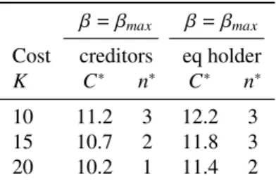
We now study numerical implications of our model on the default and renegotiation decisions, firm value, capital structure and the number of renegotiations. Regarding parameter values, we choose orders of magnitude similar to those assumed by previous models of debt renegotiation, in order to facilitate comparison between models. For our baseline case, we set the riskless interest rate to 6% (asLeland,1994andMella-Barral and Perraudin,1997did), the tax rate to 35%, volatility to 25% (both as inLeland,1994andFan and Sundaresan,2000), bankruptcy costs to 40% (Mella-Barral and Perraudin,1997chose 20%, whileLeland,1994chose 50%) and we consider a coupon rate of 7%. Without loss of generality, we set the initial assets value equal to 100. Our baseline case parameter values are presented inTable 1. These parameter values are used in all the tables and figures presented in this paper, unless specified otherwise.
Table 1: Parameter values for the baseline case Parameter Value V 100 r 6% τ 35% σ 25% α 40% c 7%
In order to better understand the renegotiation mechanism in this paper, we start by providing a numerical analysis for the case of one costless renegotiation. We discuss the renegotiation outcome, capital structure and the renegotiation surplus. Finally, we analyze the case of many costly renegotiations and provide a discussion on the optimal number of renegotiations.
6.1. Renegotiation outcome
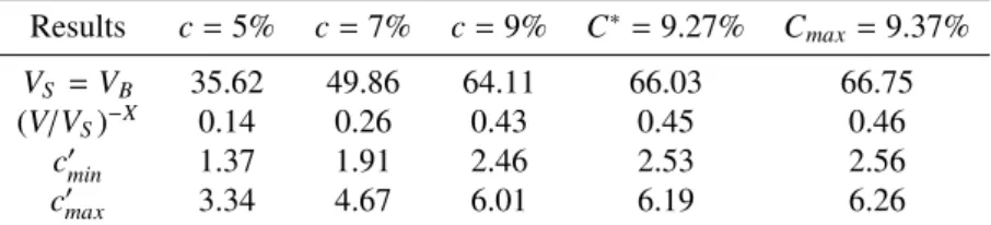
We start by examining the outcome of renegotiation at different levels of initial leverage of the firm for one costless renegotiation.Table 2illustrates the variables of interest for coupon rates varying from 5 to 9%. We present as well two special coupon rates that correspond to the optimal leverage and to the firm’s debt capacity respectively in theLeland(1994) model, i.e. C∗that maximizes the value of the firm andCmaxwhich maximizes the debt value
respectively, as defined by Leland.25 The variables we focus on are: the renegotiation thresholdV
S (which coincides
with the initial bankruptcy threshold,VB), a proxy for the probability of renegotiation (the present value of $1 to be
obtained conditional on renegotiation) and the range for the optimal reduced couponc′minandc′max.
Table 2: Numerical results of the baseline case
Results c=5% c=7% c=9% C∗=9.27% Cmax=9.37% VS =VB 35.62 49.86 64.11 66.03 66.75 (V/VS)−X 0.14 0.26 0.43 0.45 0.46 c′ min 1.37 1.91 2.46 2.53 2.56 c′ max 3.34 4.67 6.01 6.19 6.26
As shown inTable 2, the renegotiation threshold varies from 36 to 67 when we vary the coupon rate from 5% to the coupon corresponding to the firm’s debt capacity of 9.37%. The higher is the coupon they have to pay, the less is the equity holder willing to continue running the firm at this coupon level. The renegotiation probability increases with the coupon level, reaching almost 50% for a coupon as high as 9%. In all the cases the coupon is reduced at most to 27% and at least to 67% of the initial coupon value.26 The results suggest that it is precisely because of the
huge decrease in coupon that the equity holder obtains at this renegotiation threshold that she chooses to pay the full coupon until reachingVB, and does not renegotiate earlier. An earlier renegotiation would imply a smaller decrease
in the coupon value.
Fig. 2illustrates the maximum and the minimum coupon reduction for different values of volatility and bankruptcy costs. We can see that for low volatility levels the coupon range is tight, while as volatility increases this range for the new coupon widens. The coupon will be reduced at least to 86% of the initial coupon level and at most to 54% for
σ=0.1 andα=0.1. For very risky firms, withσ=0.5 andα=0.9, the coupon is reduced at least to 46% and at most to 3% of the initial level. Of course, these are extreme values, but they serve for an illustrative purpose.
25Note that the optimal coupon and the coupon that corresponds to the firm’s debt capacity in this model are in general different from those from
Leland’s model.
0 0.5 1 0.1 0.2 0.3 0.4 0.5 0 0.2 0.4 0.6 0.8 1 α σ c‘/c
Figure 2: Maximum versus minimum coupon reduction (one costless renegotiation). Relative coupon valuec′/cas a function of business (σ) and
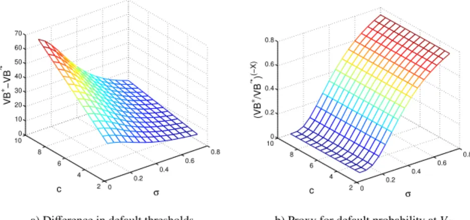
financial risk (α). The upper surface represents the minimum coupon reduction, where creditors have all bargaining power. The bottom surface represents the maximum coupon reduction, where the equity holder has all bargaining power and the coupon is reduced to the minimum value accepted by creditors. 0 0.2 0.4 0.6 0.8 2 4 6 8 10 0 10 20 30 40 50 60 70 σ c VB ∗−VB ′ * 0 0.2 0.4 0.6 0.8 2 4 6 8 10 0 0.2 0.4 0.6 0.8 σ c (VB ∗/VB ′ *) (−X)
a) Difference in default thresholds b) Proxy for default probability atVS
Figure 3: Extra life due to renegotiation (one costless renegotiation). The plots are presented as a function of the initial couponcand volatility
σ, given by two distinct measures. In panel a) the distance between the Leland default thresholdVBand the post-renegotiation default threshold V′
Bis plotted. Panel b) represents the present value (at renegotiation, when the asset value equalsVB) of $1 to be obtained conditional on default post-renegotiation, when the asset value reachesV′
B.
We finally offer further insights on the renegotiation’s outcome and effects inFig. 3, for the case of the maximum coupon reduction. We provide two distinct measures of the “extra life” that the firm obtains through renegotiation: the difference between the two default thresholds and a proxy for the probability of default at renegotiation.27 The difference between the two default thresholds plotted in panel a) ofFig. 3is logically a linear increasing function ofc
for a given volatility (asc′is proportional toc). For a given coupon level, this distance is decreasing in volatility. The
proxy for the default probability plotted in panel b) increases with volatility. Of course, the lower this probability is, the higher the extra life of the firm.
6.2. Optimal capital structure
We now study the impact of renegotiation on debt, equity, and firm value, as well as on the optimal capital structure at time 0. We plot inFig. 4debt, equity and firm value for Leland’s model (panel a)) and for our model with a single costless renegotiation, the case of maximum coupon reduction withβ=1 (panel b)). As shown inFig. 4(panel b)), in this model debt is a hump-shaped function of the coupon, and equity is a U-shaped function of the coupon. Debt
27This is not exactly the default probability, as it includes the discount factor. It is in fact the present value (at renegotiation) of $1 to be obtained
conditional on default post-renegotiation.