Proposal to Sliding Window-based Support Vector Regression

(1)

Procedia Computer Science 35 ( 2014 ) 1615 – 1624

Peer-review under responsibility of KES International. doi: 10.1016/j.procs.2014.08.245

ScienceDirect

18

th

International Conference on Knowledge-Based and Intelligent

Information & Engineering Systems - KES2014

Proposal to sliding window-based support vector regression

Yuya Suzuki

a

, Hirofumi Ibayashi

a

, Yukimasa Kaneda

b

, Hiroshi Mineno

a

*

a_{Graduate School of Informatics, Shizuoka University, 3-5-1 Johoku, Nkaka-ku, Hamamatsu, Shizuoka 432-8011, Japan} b_{Faculty of Informatics, Shizuoka University 3–5–1 Johoku, Hamamatsu, 432–8011 Japan}

Abstract

Thispaper proposes a new methodology, Sliding Window-based Support Vector Regression (SW-SVR), for micrometeorological data prediction. SVR is derived from a statistical learning theory and can be used to predict a quantity forward in time based on training that uses past data. Although SVR is superior to traditional learning algorithms such as Artificial Neural Network (ANN), it is difficult to choose the suitable amount of training data to build an optimum SVR model for micrometeorological data prediction. This paper revealed the periodic characteristics of micrometeorological data and evaluated SW-SVR can adapt the appropriate amount of training data to build an optimum SVR model automatically using parallel distributed processing. The future prediction experiment was conducted on air temperature of Sapporo, Tokyo, Hamamatsu, and Naha. As a result, SW-SVR has improved prediction accuracy in Sapporo, and Tokyo. In addition, it has reduced calculation time by more than 96 % in all regions.

Keywords:Support vector regression (SVR); Micrometerological data prediction; Agriculture

1.Introduction

Some kinds of sensor network-based agricultural support systems that enable users to monitor and control the environment in greenhouse horticulture or fields have been studied and developed1-6_{. It is difficult for farmers to}

decide and set the control parameters properly and control equipment based on priority and symptom diagnosis to cultivate high-quality plants and also set the state of these plants in a changing environment. Although model

* Corresponding author. Tel.: +81-53-478-1491; fax: +81-53-478-1491.

E-mail address: yuya@minelab.jp

(2)

predictive control (MPC) in industry is an effective means to deal with multivariable constrained control problems, a key issue for controlling the environment appropriately is how to develop the precise prediction model for micrometeorological data, such as air temperature, moisture, amount of CO2, and soil moisture, so as to cultivate plants efficiently.

The classical statistical procedures as well as artificial neural networks (ANNs) have already been applied for predicting micrometeorological data7-12_{. ANNs appear as useful alternatives to traditional statistical modeling in}

many scientific disciplines. They are composed of a large number of possible non-linear functions, or neurons, each with several parameters that are fitted to data through a computationally intensive training process. Although ANNs have good abilities for non-linear regression, they also have some drawbacks. The algorithms cannot avoid being stuck in a local optimum, which can lead to a sub-optimal solution. Besides, it is difficult to obtain the structure of a network in advance. Therefore, the network have to be optimized by considering, for example, how many neurons and hidden layers would be necessary, what kind of activation functions would be appropriate, and how to connect the neurons with each other to form a network.

Another alternative learning method that has been applied for time series prediction is support vector regression (SVR). The SVR algorithm is an extension of the popular classification method, the support vector machine (SVM). The basic idea is to adjust the possible hypotheses with linear regression by considering the width of the margin of the regression plane. By applying implicit mapping via a kernel function, SVR redefines the dot product in the linear regression method. We need to choose a proper kernel function from a small set and maintain some additional parameters for the chosen kernel function. Although several papers suggest that SVR performs well in many time series prediction problems13-17_{, it is difficult to choose the most suitable amount of training data to build the}

optimum SVR model for micrometeorological data prediction.

The aim of this paper is to reveal the periodic characteristics of micrometeorological data and the appropriate amount of training data to build the optimum SVR model. Furthermore, this paper shows that it is possible to improve both the prediction accuracy and the calculation time by choosing the appropriate training period.

The remainder of this paper is organized as follows. Section 2 show related work in meteorological data prediction. The basic idea of SW-SVR is described in section 3. Experimental environment for evaluating SW-SVR is showed in section 4. Section 5 depicts the result of evaluation experiment. Conclusion is finally made in section 6.

2.Related work

2.1.Overview

Researchers have investigated accurate environmental prediction using, for example, ANNs and SVR9-19_{. The}

ANN is a popular data modelling algorithm that mimics the operation of neurons in the human brain. It is used to express complex functions that conduct nonlinear mapping from

J to

k, where J and K are the dimensions of the input and output space, respectively20_.

The SVR algorithm is an extension of the popular classification algorithm, support vector machine (SVM)21-25_.

The SVM is a machine learning algorithm developed by Vapnik and his co-workers26_{. In SVM's original form, the}

SVM was designed to be used as a classification tool. On its introduction, researchers applied it to classification problems such as optical character recognition and face detection27-30_{. Subsequently, this algorithm was extended to}

the case of regression or estimation and termed SVR.

The SVM avoids the local extreme value problem that occurs in the ANN. The SVM replaces traditional empirical risk with structure risk minimization and solves the quadratic optimization problem that can theoretically obtain the global optimal solution16_.

2.2.Artificial neural network

ANN models have been used for air prediction9-14_{. Kadu et al.}9_{implemented air prediction in a project where they}

used Statistica software to provide the Statistica artificial neural network (SANN) (which was used here for air temperature prediction) and heavy weather software (which was used for data gathering). As a result, the ensemble networks could be trained effectively without excessively compromising the performance. The ensembles could

(3)

achieve good learning performance because one of the ensemble's members was able to learn from the correct learning pattern even though the patterns were statistically mixed with erroneous learning and Communications, and JSPS Grant-in-Aid for Challenging Exploratory Research 26660198patterns.

The original ANN air temperature models of Jain et al.11_{were developed using NeuroShell}21_{. This method was}

limited to 32,000 training patterns due to software constraints. Smith et al.12 overcame this limitation by implementing a custom ANN suite in Java. In addition, several enhancements were made to the original approach, which included the addition of seasonal variables, extended duration of prior variables, and use of multiple instantiations for parameter selection.

2.3.Support vector regression

SVR models have also been used for various weather predictions15-18_{. Liu et al.}16_{proposed the new wavelet-SVM}

model that can obtain more detailed information contained in the time series process and produce better prediction results. Therefore, it is not rigorous to predict a future trend using SVM regression in these processes. Regression on wavelet coefficients based on SVM on different scales on a time series that fully considers the impact of regularity for the time series on various scales and at various frequencies has been presented. The problem that was caused by continuous wavelet transform in the discrete time series has been solved through wavelet transform. This result indicates that the prediction accuracy obtained from the SVM method based on wavelet transform is significantly higher than that based on SVM and BP models. Chevalier et al.17_{built an SVR short-term air temperature prediction}

model and proposed a method for reducing training data. This method offers a quick means of producing reduced training data from a large amount of training data. It works by repeatedly and randomly sampling from the complete training set. Candidate training sets are quickly evaluated by applying the SVR algorithm with relaxed parameter settings, which reduces training time. The more time-consuming SVR experiments are only performed after an appropriate reduced set has been indented. Even with computational limitations on the number of training patterns that the SVR algorithm was able to handle, it produced results that were comparable and in some cases more accurate than those obtained with ANNs. Mori et al.18_{predicted daily maximum air temperature. This proposal}

method used SVR and reduced the average prediction error of a one-day-ahead maximum air temperature by 0.8% compared to that of the ANN.

3.SW-SVR (Sliding window-based support vector regression)

3.1.Overview

This paper proposes sliding window-based support vector regression (SW-SVR) for air temperature prediction. Although there are many meteorological data prediction methods using ANN and SVR that focus on improving learning speed, building a general purpose prediction model, and removing unnecessary training data, there is no research that has focused on determining the best amount of training data. Since meteorological data has four seasons, the characteristics change according to the time elapsed. Thus, it is necessary for the data in chronological order to choose the appropriate amount of training data for building a prediction model that has high prediction accuracy.

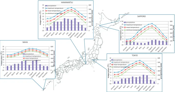
For example, Figure 1 shows meteorological characteristics of the four regions in Japan. It describes the climatic conditions of each region: maximum air temperature, mean air temperature, minimum air temperature, and precipitation. Since Japan has four seasons, the characteristics of the climate change depending on the time of year. For example there is the difference of mean temperature with January and August approximately 25 °C in Sapporo. Therefore in the case of time series prediction, the characteristics of data changes by time course. Accordingly, it is necessary to determine the appropriate amount of training data. Because over fitting is caused by building a predicting model using training data that have difference characteristics between the time of training data and the time of prediction time. To solve this problem, SW-SVR that can automatically choose the best amount of training data is proposed.

(4)

SAPPORO TOKYO HAMAMATSU NAHA 0 100 200 300 400 500 600 -10 -5 0 5 10 15 20 25 30 pr ecipitation [m m ] tem p eratur e [ ΥΥ ] precipitation maximum temperature mean temperature minimum temperature 0 100 200 300 400 500 600 -10 -5 0 5 10 15 20 25 30 35 pr ecipitation [m m ] tem p eratur e [ ΥΥ ] precipitation maximum temperature mean temperature minimum temperature 0 100 200 300 400 500 600 -10 -5 0 5 10 15 20 25 30 35 pr ecipitation [m m ] tem peratur e [ ΥΥ ] precipitation maximum temperature mean temperature minimum temperature 0 100 200 300 400 500 600 -10 -5 0 5 10 15 20 25 30 35 pr ecipitation [m m ] tem p eratur e [ ΥΥ ] precipitation maximum temperature mean temperature minimum temperature

Fig. 1. Meteorological characteristics of four regions

A Time B C D Target Predict W indow 1 10:00 10:30 11:00 11:30 12:00 12:30 13:00 13:30 14:00 14:30 15:00 Predict W indow N 10:00 10:30 11:00 11:30 12:00 12:30 13:00 13:30 14:00 14:30 15:00 䞉䞉䞉

Compare each prediction value with the actual value after the measurement period

Select the window size and parameter with the best accuracy

Rep

ea

t

A

Time B C D Target

(5)

3.2.Proposal method

Figure 2 depicts the overview of SW-SVR processing.SW-SVR can adapt the appropriate amount of training data to build the optimum SVR model using parallel distributed processing. Firstly SW-SVR divided training data into N, and builds prediction models using each divided data by parallel distributed processing. Thereafter SW-SVR evaluates each prediction models, and adopts a model with the highest prediction accuracy. Finally SW-SVR evaluates a selected prediction model used by real-time data. In time series prediction, it is possible to compare a prediction value with a measured value by time course. A prediction value and a measured value are compared sequentially, and if a difference between a prediction value and a measured value exceeds a threshold, the SW-SVR method rebuilds a prediction model. By above mentioned processing, SW-SVR keeps high-precision predicting model constantly. Figure 3 shows the detailed SW-SVR algorithm. The SW-SVR algorithm consists of four phases: x (1) Training data input phase

x (2) Dispersion characteristic evaluation phase x (3) Amount of training data selection phase x (4) Training data evaluation phase

3.2.1.Training data input phase

This phase get training data, and divided it into N. The value of N can be defined by SW-SVR users. SW-SVR evaluates each divided data by parallel distributed processing, and determines the appropriate amount of training data to build the optimum prediction model.

3.2.2.Dispersion characteristic evaluation phase

This phase investigates a dispersion characteristic of air temperature in each divided data. As for time series data such as air temperature, the data characteristics change by time course. In addition, air temperature change in Japan is the annual change. Since the data after four seasons has almost the same characteristics as the data before the four seasons, the dispersion of the air temperature tends to converge. Therefore it is suggested that the prediction accuracy of the model based on data that is older than about one year will hardly change even if the prediction model is trained with new input data.

(2) Dispersion characteristic evaluation phase

START

Get Training Data[1:nk]

Get Training Data[1:n1] Get Training Data[1:nk]

Check the Dispersion of

Objective Value [1:n1]

Check the Dispersion of

Objective Value [1:nk]

Select Training Data to

use[1:nj]

(j 䵐k)

Evaluate Prediction Model

Used Training Data[1:n1]

Evaluate Prediction Model

Used Training Data[1:nj]

Select Best Training Data

[1:nj] (j 䵐k)

Build Model

Open Test Using Real time data Accuracy is less than

a threshold value

NO

YES

䞉䞉䞉

(1) Training data input phase

(3) Amount of training data selection phase

(4) Prediction model evaluation phase

(6)

Hence, to select the amount of training data, it is important to determine it before the variance of air temperature converges. This phase detects a convergence of dispersion value in air temperature using change of a differentiation value of a dispersion value. Figure 4 shows the example of dispersion characteristic detection. A differentiation value of a dispersion value in divided data is compared with a threshold that a user established. In this sample, a value of threshold is established |0.5|. SW-SVR finds a differential value between k months and k + 1 months. Thereafter, each differential value is compared with a value of threshold. If a differential value is within a threshold, and a differential value that exceeds the threshold does not appear afterword, SW-SVR defines it as convergence of a dispersion value. Finally it provides data from start until the detected period for phase (3).

3.2.3.Amount of training data selection phase

This phase builds prediction models using data constellation, and evaluate each model’s prediction accuracy. SW-SVR measures prediction accuracy in terms of root mean square error (RMSE) of ensemble average. RMSE is expressed in formula (1), where N is the number of test data and

e

_i is the error of the ensemble mean for each test data i averaged over the required spatial region. In addition,

N e N i

¦

1 2

in the formulation (1) is called mean square error (MSE). RMSE is guided by an open test that uses the test data that did not use for building prediction model. The open test evaluates the prediction accuracy of the model by using the evaluation data which is different from the training data used to build the prediction model. After this phase, appropriate prediction model that has the lowest RMSE is selected. N e RMSE N i

¦

1 2

)

1

(

-1

-0.5

0

0.5

1

1.5

2

0

2

4

6

8

10

12

1

3

5

7

9 11 13 15 17 19 21 23 25 27 29 31 33 35

Differ

ential of

variance

variance of air

tem

p

eratur

e[

Υ

]

The amount of taining data [months]

Differential Variance (ii) A value within the threshold

doesn't appear afterward

(i) Thresholds :|0.5|

(iii) Select training period

(7)

3.2.4.Prediction model evaluation phase

This phase evaluates a prediction model through the open test used by real-time data. If the RMSE guided by the difference between prediction value and real-time measured value is less than a threshold value, returns to the initial processing, and rebuild a prediction model. By above mentioned processing, SW-SVR determines the best amount of training data, and keeps a high accuracy prediction model.

4.Experimental environment

4.1.Assumed condition

Since meteorological data has four seasons, the characteristics change according to the time elapsed. Thus, it is necessary for the data in chronological order to choose the appropriate amount of training data for building a prediction model that has high prediction accuracy. To evaluate SW-SVR, an experiment was conducted for the meteorological data in Japan for past three years, and used four regions where climate conditions differ.

The experiment used open meteorological data of Japan that was provided by the automated meteorological data acquisition system (AMeDAS). AMeDAS is an automated meteorological data acquisition system managed by the meteorological agency in Japan. This system provides meteorological data: air temperature, relative humidity, station pressure, precipitation, mean wind, maximum wind, relative humidity, and sunshine duration. The measurement cycle is every ten minutes.

Meteorological data of four Japanese areas, Sapporo, Tokyo, Hamamatsu, and Naha, were used as evaluation data to be evaluated objectively by using the typical weather characteristics of each different area. Meteorological data of the northernmost area (Sapporo), southernmost area (Naha), center area (Hamamatsu), and capital of Japan (Tokyo) were analyzed.Since the meteorological data was time series data and the changes in annual climate characteristics were the same, enough evaluations could be obtained by preparing training data for the past three years. The experiments were conducted on the meteorological data up to January 2, 2014, and a deficit period was removed from January 1, 2011. A deficit period means the point where a value is lost partially owing to AMeDAS sensor trouble.

4.2.Experiment contents

To evaluate SW-SVR, this experiment used meteorological data for the past three years. SW-SVR divided it into 36, and selected the appropriate amount of training data in accordance with the SW-SVR algorithm. The dependent variable is air temperature after one hour.The data from January 1, 2011 to January 1, 2014 were used for training data. Meanwhile, the data from January 2, 2014 were used for evaluation data. SW-SVR is evaluated by comparing it with SVR. An SVR model is built using all training data (36months data), and An SW-SVR model is built using selected training data. Evaluation index is prediction accuracy and calculation time that is the time required to build a prediction model.

5.Result and discussion

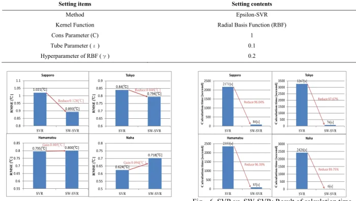
This paper evaluated SW-SVR models compared with SVR. Evaluation index is RMSE and calculation time. Since the total amount of data for three years was large (more than 158,000 items), a huge calculation time to tune SVM parameters was required. Thus, this experiment set each parameter (cost parameter C, tube parameter ε, and the hyperparameter of RBF γ) to a constant value and tested without parameter tuning, using, for example, a grid

(8)

Table 1. SVR conditions

Setting items Setting contents

Method Epsilon-SVR

Kernel Function Radial Basis Function (RBF)

Cons Parameter (C) 1 Tube Parameter (Ȝ) 0.1 Hyperparameter of RBF (Ț) 0.2 1.021[Υ] 0.893[Υ] 0.8 0.85 0.9 0.95 1 1.05 1.1 SVR SW-SVR RM S E [ Υ Υ ] Sapporo 0.84[Υ] 0.794[Υ] 0.6 0.65 0.7 0.75 0.8 0.85 0.9 SVR SW-SVR RM S E [ Υ Υ ] Tokyo 0.795[Υ] 0.800[Υ] 0.55 0.6 0.65 0.7 0.75 0.8 0.85 SVR SW-SVR RM S E [ Υ Υ ] Hamamatsu 0.624[Υ] 0.718[Υ] 0.5 0.55 0.6 0.65 0.7 0.75 0.8 SVR SW-SVR RM S E [ Υ Υ ] Naha Reduce 0.128[Υ] Reduce 0.046[Υ] Gain 0.005[Υ] Gain 0.094[Υ]

Fig. 5. SVR vs. SW-SVR: Result of RMSE

2171[s] 86[s] 0 500 1000 1500 2000 2500 SVR SW-SVR C a lcul a ti o n ti m e [s eco nd] Sapporo 3267[s] 76[s] 0 500 1000 1500 2000 2500 3000 3500 SVR SW-SVR C a lcul a ti o n ti m e [s eco nd] Tokyo Reduce 97.67% 2353[s] 85[s] 0 500 1000 1500 2000 2500 SVR SW-SVR C a lcul a ti o n ti m e [s eco nd] Hamamatsu 2426[s] 6[s] 0 500 1000 1500 2000 2500 3000 SVR SW-SVR C a lcul a ti o n ti m e [s eco nd] Naha Reduce 96.04% Reduce 96.39% Reduce 99.75%

Fig. 6. SVR vs. SW-SVR: Result of calculation time

Figure 5 and Figure 6 describe experimental results. Figure 5 shows the result of RMSE in each area, and Figure 6 depicts the result of calculation time. In RMSE, SW-SVR improved prediction accuracy in Sapporo, and Tokyo (reduce 0.128rC for Sapporo and 0.046rC for Tokyo). In the case of Hamamatsu, RMSE little changed (gain 0.005 Υ). On the other hand SW-SVR gained RMSE in Naha 0.094 rC. Meanwhile SW-SVR reduced a calculation time more than 96 % in all regions. SW-SVR model of Sapporo chose the past seven months amount of training data among past 12 months training data. In addition, SW-SVR model of Tokyo selected the past four months, and the model of Hamamatsu determined the past 11 months among past 11 months training data. In the case of Naha, three months training data was selected among four months training data. The value of RMSE was guided by a model used by SW-SVR choosing training data. On the other hand, the calculation time depended on the amount of the consultation period which SW-SVR determined.

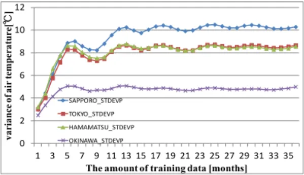
As for the reason why there were the area where predictive precision was improved and the area that were not improved is a cause in dispersion value of the temperature. Figure 7 shows RMSE transitions for air temperature, and Figure 8 depicts transitions for air temperature dispersion value. Both figures show that the largest value was Sapporo, followed in order by Tokyo, Hamamatsu and Naha. The volume of a dispersion value means the size of the change of the air temperature of one year. Thus past data work as a noise data. Accordingly the over fitting is caused by training past data. Hence Sapporo that has large dispersion value of air temperature has a tendency to increase

(9)

0.5 0.6 0.7 0.8 0.9 1 1.1 1 3 5 7 9 11 13 15 17 19 21 23 25 27 29 31 33 35 R M SE[ Υ Υ ]

The amount of training data [months] RMSE_Sapporo

RMSE_Tokyo RMSE_Hamamatsu RMSE_Naha

Fig. 7. RMSE transitions for air temperature

0 2 4 6 8 10 12 1 3 5 7 9 11 13 15 17 19 21 23 25 27 29 31 33 35 var ian ce of air te mp er at ur e[ Υ Υ ]

The amount of training data [months] SAPPORO_STDEVP

TOKYO_STDEVP HAMAMATSU_STDEVP OKINAWA_STDEVP

Fig. 8. Dispersion value transitions for air temperature

RMSE by time course. Therefore the concept of SW-SVR was effective in the area that has large dispersion value such as Sapporo.

Consequently this experiment showed that SW-SVR could improve prediction accuracy in the area that has large dispersion value of air temperature, and reduce calculation time in all area. If SW-SVR is assumed using an application for agriculture, the prediction model must have both high prediction accuracy and calculation speed. Since there is a possibility that a sudden environmental change occurs in agricultural environments, farmers should work while they predict the change of the environment at all times. Accordingly, SW-SVR can be used for implementing an agricultural support application.

Conclusion and future work

In this paper, SW-SVR that is a new methodology for micrometeorological data prediction was proposed. In time series air-prediction, since the meteorological data characteristics change according to the time elapsed, past data work as a noise data. Thus, it is necessary to determine the suitable amount of training data for building prediction model. SW-SVR can determine the appropriate amount of training data to build more optimum SVR model automatically using parallel distributed processing. The experiments show that the proposed was successfully to determine the suitable amount of training data in the meteorological data of the year to January1, 2014 from January1, 2011 in Sapporo, Tokyo, Hamamatsu, and Naha provided by AMeDAS. SW-SVR could improve RMSE in Sapporo, and Tokyo. In addition, it could reduce calculation time in all area. The remaining issues are evaluating more various situations to show SW-SVR works useful. In this paper, SW-SVR was evaluated using only air temperature.

Acknowledgements

This study was partially supported by the budget for 2013 Strategic Information and Communications R&D Promotion Programme (SCOPE), Ministry of Internal Affairs and Communications, and JSPS Grant-in-Aid for Challenging Exploratory Research (26660198), Japan.

References

1. Kang, B, Park, D, Cho, K, Shin, C, Cho, S, & Park, J "A study on the greenhouse auto control system based on wireless sensor network," Security Technology, SECTECH'08, International Conference on IEEE, pp41-44, 2008.

2. Pierce, F. J, and T. V. Elliott. "Regional and on-farm wireless sensor networks for agricultural systems in Eastern Washington," Computers and electronics in agriculture 61.1, pp32-43, 2008.

(10)

3. Gonda, Luciano, and Carlos Eduardo Cugnasca, "A proposal of greenhouse control using wireless sensor networks," Proceedings of 4thWorld Congress Conference on Computers in Agriculture and Natural Resources, Orlando, Florida, USA, 2006.

4. Ahonen, Teemu, Reino Virrankoski, and Mohammed Elmusrati. "Greenhouse monitoring with wireless sensor network," Mechtronic and Embedded Systems and Applications, 2008, MESA 2008, IEEE/ASME International Conference on IEEE, 2008.

5. Hori, Mitsuyoshi, Eiji Kawashima, and Tomihiro Yamazaki, "Application of Cloud computing to agriculture and prospects in other fields," Fujitsu Sci, Tech, J 46.4, pp446-45, 2010.

6. Wang, Ning, Naiqian Zhang, and Maohua Wang, "Wireless sensors in agriculture and food industry-Recent development and future perspective," Computers and electronics in agriculture 50.1, pp1-14, 2006.

7. Bennett, Kristin P, and Olvi L. Mangasarian, "Robust linear programming discrimination of two linearly inseparable sets," Optimization methods and software 1.1, pp.23-34, 1996.

8. Fletcher, Roger, "Practical methods of optimization," John Wiley & Sons, 2013.

9. Kadu, Parag, Kishor Wagh, and Prashant Chatur, "Analysis and Prediction of Air temperature using Statistical Artificial Neural Network," International Journal of Computer Science 12, pp117-122, 2012.

10. Roebber, P, Butt, M. and Reinke, S, "Real-time forecasting of snowfall using a neural network," Weather Forecasting, Vol.22, pp.676-684, 2007.

11. Jain, A, R. W. McClendon, and G. Hoogenboom, "Freeze prediction for specific locations using artificial neural networks," Transactions of the ASABE 49.6, pp1955-1962, 2006.

12. Smith, Brian A, Gerrit Hoogenboom, and Ronald W. McClendon, "Artificial neural networks for automated year-round air temperature prediction," Computers and Electronics in Agriculture 68.1, pp.52-61, 2009.

13. Smith, Brian A., Ronald W. McClendon, and Gerrit Hoogenboom, "Improving air temperature prediction with artificial neural networks," International Journal of Computational Intelligence 3.3, pp.179-186, 2006.

14. CHEN Renfang, and LIU Jing, "The Area Rainfall Prediction of Up-river Valleys in Yangtze River Basin on Artificial Neural Network Modes", Scientia Meteorologica Sinica, 24(4), pp483-486, 2009.

15. Gill, M, Asefa, T, Kemblowski, M. and McKee, M, "Soil moisture prediction using support vector machines," Journal of the American Water Resources Association, Vol.42, pp.1033-1046, 2006.

16. Liu, Xiaohong, Shujuan Yuan, and Li Li, "Prediction of Air temperature Time Series Based on Wavelet Transform and Support Vector Machine," Journal of Computers 7.8 ,pp1911-1918 2012.

17. Chevalier, R. F, Hoogenboom, G, McClendon, R. W, & Paz, J. A, "Support vector regression with reduced training sets for air temperature prediction: a comparison with artificial neural networks," Neural Computing and Applications 20.1, pp.151-159, 2011.

18. Mori, Hiroyuki, and Daisuke Kanaoka, "Application of support vector regression to air temperature forecasting for short-term load forecasting," Neural Networks, 2007, IJCNN 2007, International Joint Conference on IEEE, 2007.

19. Hua, X. G, Ni, Y. Q, Ko, J. M, & Wong, K. Y, "Modeling of air temperature-frequency correlation using combined principal component analysis and support vector regression technique," Journal of Computing in Civil Engineering 21.2, pp.60-66, 2007.

20. Engelbrecht, Andries P, "Computational intelligence: an introduction," Wiley. com, 2007. 21. Frederick, M. D, "Neuroshell 2 user's manual," 1995.

22. Smola, Alex J, and Bernhard Sch?lkopf, "A tutorial on support vector regression," Statistics and computing 14.3 pp.199-222, 2004. 23. Mattera, Davide, and Simon Haykin, "Support vector machines for dynamic reconstruction of a chaotic system," Advances in kernel

methods, MIT Press, pp.211-241, 1999.

24. Vapnik, Vladimir, Steven E. Golowich, and Alex Smola, "Support vector method for function approximation, regression estimation, and signal processing," Advances in neural information processing systems, pp. 281-287, 1999.

25. K. R. Müller, A. J. Smola, G. Rätsch, B. Schökopf, J. Kohlmorgen, and V. Vapnik, "Using support vector machines for time series prediction," Chemometrics and intelligent laboratory systems 69.1 pp.35-49, 2003.

26. Cortes,Corinna, and VladimirVapnik, "Support vector networks," Machine learning 20.3 pp.273-297, 1995.

27. Osuna, Edgar, Robert Freund, and Federico Girosit, "Training support vector machines: an application to face detection," Computer Vision and Pattern Recognition, 1997, Proceedings, 1997 IEEE Computer Society Conference on IEEE, 1997.

28. Ravi, S, and S. Wilson, "Face Detection with Facial Features and Gender Classification Based On Support Vector Machine," Proceedings of IEEE International Conference on Computational Intelligence and Computing Research, 2010.

29. Scholkopf, Bernhard, Chris Burges, and Vladimir Vapnik, "Incorporating invariances in support vector learning machines," Artificial Neural Networks-ICANN 96, Springer Berlin Heidelberg,pp.47-52, 1996.

30. Sun, Aixin, Ee-Peng Lim, and Ying Liu, "On strategies for imbalanced text classification using SVM: A comparative study," Decision Support Systems 48.1, pp.191-201, 2009.