Bargaining with Non-convexities

P. Jean-Jacques Herings, Arkadi Predtetchinski

Bargaining with Non-convexities RM/09/042

Bargaining with Non-convexities

P. Jean-Jacques Herings

Arkadi Predtetchinski

October 8, 2009

Abstract

We show that in the canonical non-cooperative multilateral bargaining game, a sub-game perfect equilibrium exists in pure stationary strategies, even when the space of feasible payoffs is not convex. At such an equilibrium there is no delay. We also have the converse result that randomization will not be used in this environment in the sense that all stationary subgame perfect equilibria do not involve randomization on the equilibrium path. Nevertheless, mixed strategy profiles can lead to Pareto superior payoffs in non-convex cases.

Keywords: Bargaining, non-convexities, stationary subgame perfect equilibrium,

existence, pure strategies.

JEL codes: C62, C72, C73, C78.

∗_{P.J.J. Herings, Department of Economics, Maastricht University, P.O. Box 616, 6200 MD, Maastricht,}

The Netherlands. This author would like to thank the Netherlands Organization for Scientific Research (NWO) for financial support. [email protected]

†_{A. Predtetchinski, Department of Economics, Maastricht University, P.O. Box 616, 6200 MD,}

Maas-tricht, The Netherlands. This author would like to thank the Netherlands Organization for Scientific Research (NWO) for financial support. [email protected]

1

Introduction

Many problems in economics are complicated by the presence of non-convexities. Scarf (1994) mentions the omnipresence of non-divisibilities in production as an important source of non-convexities in economics. Another example of a non-convexities in production is the existence of production technologies with increasing returns to scale. Other important cases of non-convexities result from non-convexities in preferences, even in the presence of lotteries when agents are not expect utility maximizers as is for instance the case in prospect theory, see Kahneman and Tversky (1979), or when randomization is not possible, and non-convexities in the consumption set, for instance caused by the presence of indivisible commodities. Although non-convexities are regarded important, most of the economic literature assumes them away for reasons of intractability.

Non-convexities are frequently studied in the n-person cooperative bargaining litera-ture. There is for instance an extensive literature on the extension of the Nash bargaining solution to non-convex environments (Kaneko (1980), Conley and Wilkie (1996), Mariotti (1997), Zhou (1997), and Xu and Yoshihara (2006)). On the contrary, the literature on strategic bargaining has not paid much attention to non-convexities and non-convexities are only treated for the two-player case. Rubinstein (1982) allows for modest forms of non-convexities. Under his hypothesis there is typically a unique equilibrium. Herrero (1989) considers general non-convexities for the two-player case and obtains the existence of a subgame perfect equilibrium in stationary strategies when the set of feasible payoffs is strictly comprehensive. Conley and Wilkie (1995) also consider a strictly comprehensive set of feasible payoffs and introduce a bargaining protocol that implements their extension of the Nash bargaining solution.

Existence of a pure equilibrium in the canonical multilateral bargaining model has been shown only when the set of feasible payoffs is convex. The existence of such an equilibrium has been shown in Banks and Duggan (2000). Merlo and Wilson (1995) consider the

n-person cake division problem and obtain the existence of a unique subgame perfect equilibrium in stationary strategies when the set of feasible payoffs is convex and the proposer selection protocol is deterministic.

We consider the following canonical multilateral bargaining procedure. In each time period, nature randomly selects a player that is allowed to make a proposal. All players respond sequentially to the proposal and either vote in favor or against. As soon as a responder votes against the proposal, the procedure continues in the next period. If all responders vote in favor of the proposal, it is accepted, and the procedure ends.

The bargaining game is fully characterized by the set of players, their discount factors, the set of feasible payoffs, and the probability according to which nature selects a particular proposer. The only assumptions we make regarding the set of feasible alternatives are

non-substantial technical ones. It is assumed to be closed, comprehensive from below, and the set of individually rational payoffs is assumed bounded from above. To make the bargaining problem non-trivial, it is assumed that there is an alternative that gives all players a strictly positive payoff.

We show that this entire class of bargaining games has stationary subgame perfect equilibria in pure strategies that ensure immediate agreement. This result is surprising as the usual way to deal with non-convexities is to introduce lotteries. For that reason, one might have expected that non-convex bargaining games possess mixed strategy equilibria rather than pure ones. Similarly, one might have expected that non-convexities are a potential source for delay.

We also address the reverse question. Under what conditions are all stationary subgame perfect equilibria of a bargaining game in pure strategies without delay? The answer is that an extremely mild additional assumption assures this: When the set of weakly Pareto optimal alternatives coincides with the set of Pareto optimal ones, all stationary subgame perfect equilibria involve no randomization on the equilibrium path. Equilibria are characterized by the absence of delay.

To derive the first main result, the existence result, we deviate from the usual proof strategy that basically exploits continuity of the best-response correspondences. In our non-convex setting, this correspondence may not be continuous. Instead, we construct an excess utility function that resembles the excess demand function as used in general equilibrium theory. Let some profile of ex ante utilities be given and consider for each playeri the (potentially infeasible) proposal playerihas to make in order to be consistent with this profile of ex ante utilities. Coordinateiof the excess utility function is the degree of feasibility of this proposal. The excess utility function is shown to have a zero point by showing that it is not outward pointing. Next, a zero point is shown to induce a subgame perfect equilibrium in stationary strategies of the bargaining game.

To prove the second main result, roughly stating that all stationary subgame perfect equilibria are in pure strategies, we proceed in several steps. One of the main steps is to show in an equilibrium in mixed strategies, proposals offering strictly more than the continuation utility to all players are accepted with probability one, whereas proposals offering at least one player strictly less than the continuation utility are accepted with probability zero. The next main step is to argue that for every player there is a unique proposal which maximizes his utility subject to being accepted with probability one and that every mixed equilibrium puts probability one on such a proposal.

Equilibria are efficient in the sense that in equilibrium every proposer selects a Pareto optimal alternative. However, the fact that all equilibria are in pure strategies implies that equilibria may be inefficient in a weaker sense. It is not difficult to construct examples and

mixed strategy profiles with associated utilities strictly Pareto dominating the equilibrium utilities.

This paper is organized as follows. Section 2 introduces the model and Section 3 provides the existence result. Section 4 proves the converse result and Section 5 concludes.

2

The Bargaining Game

We consider the bargaining game Γ = (N, V, δ, θ). There is a set N of n individuals that have to select a single payoff vector in the set of feasible payoffs V, a non-empty subset of RN. We denote the set of non-negative feasible payoffs by V₊ = V ∩RN₊. The vector

δ= (δ_i)_i∈N consists of the players’ discount factors and θ= (θ_i)_i∈N denotes the probability according to which players are selected as a proposer. Individuals negotiate about the alternative to be selected using a procedure defined as follows.

In every time period t, starting with t = 0, nature selects player i to be the proposer with probability θ_i. After history h, player i makes a proposal σi(h). In Sections 2 and 3 we restrict ourselves to pure strategies, in which case σi(h) corresponds to an element in V₊. After observing σi(h), all players (including the proposer) vote sequentially on the proposal, the order of their responses being history independent. Each player can either accept or reject the proposal. If the proposal is unanimously accepted, the proposal σi(h) is implemented. As soon as the first rejection occurs, the period t+ 1 begins, with nature selecting a new proposer, and so on.

The utility to player i of agreement on v ∈ V in time period t is given by δt_iv_i. The utility of perpetual disagreement is equal to 0 for all players. Players have von Neumann-Morgenstern utility functions.

Our assumptions are as follows.

(A) The setV is closed and comprehensive from below. The setV₊is bounded and contains 0 in its interior.

(B) The discount factor δ_i belongs to [0,1) for all i.

We analyze the stationary subgame perfect equilibria (SSPE) of Γ. A stationary strategy

of individualispecifies a proposal xi and anindividual acceptance set Ai. At every history

h where player i is selected as a proposer, he makes the proposal σi(h) =xi and at every history h where player i has to respond, he accepts the proposal currently on the table if and only if it belongs toAi. A strategy profile is a stationary subgame perfect equilibrium

if it is stationary and if it induces a Nash equilibrium in every subgame.

The main existence result for this model is Theorem 2 in Banks and Duggan (2000). This theorem states that when the set of feasible payoffs is convex, then there exists a pure

strategy no-delay stationary equilibrium. Moreover, they have the converse result that every no-delay stationary equilibrium is in pure strategies when the set of feasible payoffs is strictly convex. We show that for an existence result, it suffices to make assumptions (A) and (B). It follows in particular that convexity assumptions are not needed. Under the modest additional assumption that weakly Pareto efficient and Pareto efficient points co-incide, we obtain the converse result that every stationary equilibrium uses pure strategies on the equilibrium path and does not involve delay.

3

Existence of Stationary Subgame Perfect Equilibria

in Pure Strategies

In this section we present a system of equations which is such that a solution to the system induces an SSPE in pure strategies. Let g :RN → R be a transformation function, i.e. a function such thatv ∈V if and only if g(v)≥0, with v∈∂V if and only if g(v) = 0.

Assumption A1 can be rephrased in terms of g. It is evident that A1 is equivalent to the existence of a transformation function g satisfying the following conditions:

• g is continuous, • g(0N)>0,

• g(ˆv)≥0 andv ≤vˆimplies g(v)≥0,

• g−1(R₊)∩RN₊ is bounded.

Let u ∈ RN be a vector of ex ante expected utilities for the players. Consider the case where for every playerihis proposalxi is immediately accepted and satisfies g(xi) = 0 and

xi_j = δ_ju_j for j = i. Player i is the proposer with probability θ_i and is a responder with probability 1−θ_i,so consistency with ex ante expected utility imposes

u_i=θ_ixi_i+ (1−θ_i)δ_iu_i.

By rearranging terms we obtain that

xi_i = 1−δi+θiδi

θ_i ui.

For i∈N, we define α_i = (1−δ_i+θ_iδ_i)/θ_i and we define the function pi :RN →RN by

pi_j(u) =

α_iu_i, ifj =i, δ_ju_j, ifj ∈N\ {i}.

The function pi specifies the proposals that are consistent with ex ante expected utilities

u.

Let ¯v ∈RN₊₊ be a strict upper bound onV₊, so every v∈V₊ satisfies v≤¯v.

We define the functionz : [0N,v¯]→RN as follows:

z_i(u) =g(pi(u)), i∈N.

If z_i(u)<0,then there is no payoff vector in the set of feasible payoffs that gives player i

a payoff of α_iu_i and players j = ia payoff of δ_ju_j.Consistency with ex ante utilities would impose thatu_i be lowered. Ifz_i(u)>0,then there is a payoff vector inV that gives player

i a payoff of strictly more than α_iu_i and players j = i a payoff of δ_ju_j. In this case it is possible to increase u_i.

The function z is related to an excess demand function as used in general equilibrium theory and we can think of z as an excess utility function. To find equilibria in pure strategies, we are looking for solutions to the system of equations z(u) = 0N. Notice that the system of equations z(u) = 0N is different from the usual one (see Merlo and Wilson (1995), Banks and Duggan (2000), Kalandrakis (2004, 2006)), where typically each player is maximizing his utility subject to meeting the reservation values. Our assumptions do not imply that the system of equations employed in the usual approach is continuous.

A function isoutward pointing at a pointif the function value is a non-zero element of the normal cone at the point. A function is outward pointing if it is outward pointing at some point. When applied to a function f : [a,¯a]→ Rm,where [a,¯a] is the m-dimensional unit interval witha ¯a,we obtain the following definition.

Definition 3.1 Let a,a¯ in Rm be such that a a.¯ The function f : [a,¯a] → Rm is outward pointing at a∈[a,¯a] if f(a)= 0 and, for k= 1, . . . , m, a_k =a_k implies f_k(a)≤0, a_k < a_k <¯a_k implies f_k(a) = 0,anda_k = ¯a_k impliesf_k(a)≥0.

We show next that the excess utility functionz is not outward pointing.

Lemma 3.2The excess utility function z is not outward pointing.

Proof: Clearly, z is not outward pointing at anyu in the interior of [0N,¯v].

Consider u in the boundary of [0N,v¯] and i ∈ N such that u_i = ¯v_i. Then, since

pi(u)∈RN₊ and there is no v∈V₊ with v_i =α_iv¯_i> ¯v_i,we have that

z_i(u) =g(pi(u))<0.

Therefore z is not outward pointing at such a pointu.

Consider u in the boundary of [0N,¯v] such that u ¯v and u_i = 0 for at least one i ∈ N. Suppose that z is outward pointing at u. Clearly u = 0N, since z(0N) =

(g(0N), . . . , g(0N)) 0N. Let j be such that 0 < u_j < v¯_j. Then, since z is outward pointing atu,

0 =z_j(u) =g(pj(u)),

so pj(u) ∈ V. Since pj(u) > pi(u) for any i ∈ N such that u_i = 0, we have pi(u) ∈V, so

z_i(u) =g(pi(u))≥0. Since z is outward pointing atu it follows thatz_i(u) = 0 for every i

such that u_i= 0.We find that z(u) = 0,a contradiction toz being outward pointing atu.

Q.E.D.

Functions that are not outward pointing have a zero point.

Lemma 3.3Let a,¯a in Rm be such that aa¯and let the function f0 : [a,¯a]→ Rm be not outward pointing. Then f0 has a zero point.

Proof: We define the function f1: [a−1m,¯a+ 1m]→ Rm by

f1(a) =λ(a)(π_[a,a¯](a)−a) + (1−λ(a))f0(π_[a,¯a](a)), a∈[a−1m,¯a+ 1m],

where π_[a,a¯] is the orthogonal projection function on [a,¯a] and

λ(a) =π_[a,¯a](a)−a_∞, a∈[a−1m,¯a+ 1m],

so the function λ : [a−1m,¯a+ 1m] → [0,1] measures the distance in infinity norm from the point a to its projection. The function λ is continuous and has the property that it is equal to 1 on the boundary of [a−1m,¯a+ 1m],equal to 0 on [a,¯a],and strictly in between 0 and 1 everywhere else. We define the functionf2 : [a−1m,¯a+ 1m]→ [a−1m,¯a+ 1m] by

f2(a) =π_[a−1m_,a¯+1m_](a+f1(a)), a∈[a−1m,a¯+ 1m].

The function f2 has a fixed point, say a∗, by Brouwer’s fixed point theorem. Suppose a∗ belongs to the boundary of [a−1m,¯a+ 1m],i.e. λ(a∗) = 1. Then

a∗ =f2(a∗) =π_[a−1m_,¯a+1m_](a∗+f1(a∗)) =π_[a−1m_,a¯+1m_](a∗+π_[a,¯a](a∗)−a∗) =π_[a,¯a](a∗)=a∗,

a contradiction. It follows that a∗ is not in the boundary of the set [a−1m,¯a+ 1m], i.e. it belongs to its relative interior. From this it follows that

a∗= π_[a−1m_,¯a+1m_](a∗+f1(a∗)) =a∗+f1(a∗),

so f1(a∗) = 0m. Using the definition off1 it then follows that

f0(π_[a,¯a](a∗)) =− λ(a

∗₎

1−λ(a∗)(π[a,¯a](a

Now ifa∗ is not an element of the set [a,¯a], then 0< λ(a∗)< 1 and the vectora∗−π_[a,¯a](a∗) is a non–zero element of the normal cone of [a,a¯] at the point π_[a,¯a](a∗). But this means that f0 is outward pointing at π_[a,¯a](a∗), a contradiction. We conclude that a∗ ∈ [a,a¯]. Thus λ(a∗) = 0 and π_[a,¯a](a∗) =a∗, so a∗ is a zero point of the function f0. Q.E.D.

Corollary 3.4The excess utility function z has a zero point.

A zero point u∗ of z induces a subgame perfect equilibrium in stationary strategies of Γ as follows. Fori∈N, we define

x∗i =pi(u∗),

and

A∗i= {v ∈V |v_i > δ_iu∗_i} ∪ {v∈V |v_i=δ_iu∗_i and∀j =i, v_j ≤α_ju∗_j)}.

Whenever a playerihas to propose, he makes the proposalx∗i.Whenever a playerihas to respond, he accepts proposals that offer him strictly more utility thanδ_iu∗_i or that offer him exactly δ_iu∗_i and do not offer more than α_ju∗_j for other players j. In this construction we exploit the degree of freedom that we have in case a player is indifferent between accepting and rejecting a proposal. This freedom is needed in particular when the set V contains points that are only weakly Pareto optimal as Example 3.6 illustrates. Indeed, it may well be that a proposal that maximizes the proposer’s utility subject to offering the other play-ers their reservation values is not compatible with an equilibrium. Equilibrium play may require a proposer to settle for a weakly Pareto optimal proposal that is not Pareto optimal.

Theorem 3.5The strategy profile (x∗, A∗) is an SSPE of Γ.

Proof: It is well-known that the game Γ has the one-shot deviation property, meaning

that if there is a subgame where a player has some profitable deviation from a stationary strategy profile, then there must also be a subgame where this player has a profitable one-shot deviation, i.e. a single deviation by this player at the root of the subgame. A minor extension of the arguments in Fudenberg and Tirole (1991) would prove this point.

We verify that no player has a profitable one-shot deviation. Suppose at some historyh

at time period t,playeriis proposer and makes proposalxi,potentially different fromx∗i.

Notice that x∗i is accepted leading to expected utility δt_iα_iu∗_i for playeri. If xi ∈ ∩_i∈NA∗i,

then it will be rejected, leading to an expected utility of δt_i+1u∗_i < δ_itα_iu∗_i.If xi ∈ ∩_i∈NA∗i

it will be accepted, leading to a utility of δ_itxi_i. Since xi ∈ A∗j for j = i, it follows that

xi_i ≤ α_iu∗_i, so the expected utility to player i of proposing xi is less than or equal to the expected utility of proposing x∗i.

Suppose at some historyhat time periodt,playeriis responder to a proposal v∈A∗i.

In equilibrium, player i accepts. The expect utility to player i is δ_itv_i if the other players accept and δt_i+1u∗_i if some other player rejects, so expected utility weakly exceeds δ_it+1u∗_i

in any case. Would playeri deviate to a rejection, then his expected utility equals δt_i+1u∗_i.

Consider a proposal v ∈ A∗_i, so in particular v_i ≤ δ_iu∗_i. In equilibrium, player i rejects, leading to expected utilityδ_it+1u∗_i. A deviation to acceptance leads to expected utility δt_iv_i

if others accept and δ_it+1u∗_i if some other player rejects. In either case, expected utility is

bounded above by δ_it+1u∗_i. Q.E.D.

Example 3.6Consider the set of feasible payoffs

V ={v ∈R2 |v₁ ≤2, v₂ ≤2, max{v₁, v₂} ≤1},

which is depicted in Figure 1. An upper bound on V₊ is given by ¯v = (2,2).

-6 0 1 2 v₁ 0 1 2 v₂ V

Figure 1: The set of feasible payoffs

Players are selected as proposer with equal probability, so θ₁ = θ₂ = 1/2. It follows that α_i = 2−δ_i.The excess utility function z is then defined by

z₁(u) = g(p1(u)) = g((2−δ₁)u₁, δ₂u₂), u∈[0,v¯]

z₂(u) = g(p2(u)) = g(δ₁u₁,(2−δ₂)u₂), u∈[0,v¯].

The boundary of V consists of four types of line segments, characterized by v₁ ≤ 1 and

v₂ = 2, v₁ = 1 and 1≤v₂ ≤2, 1≤v₁≤2 and v₂ = 1,andv₁= 2 and 0≤v₂ ≤1.Since in equilibrium bothp1(u) andp2(u) belong to such a line segment, there are potentially sixteen types of equilibria, where a type of equilibrium corresponds to a particular combination of line segments to which the proposal belongs. When we solve for z(u) = 0 for each of the sixteen resulting systems of equations, and taking into account that 0≤δ₁, δ₂<1,we find ex ante equilibrium utility levels u∗₁ andu∗₂.From these, we can derive the equilibrium

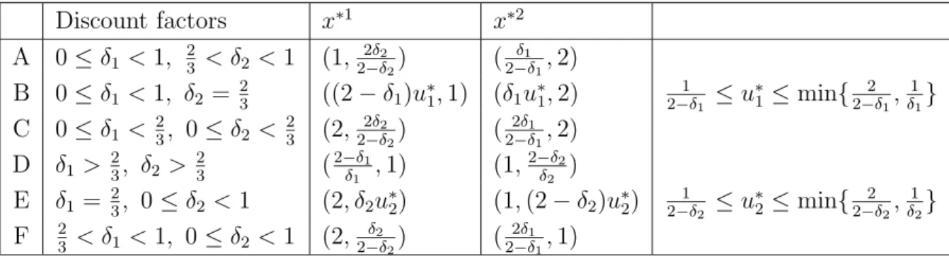
proposals x∗1 and x∗2 and the equilibrium acceptance sets A∗1 and A∗2. The equilibrium proposals are displayed in Table 3. We distinguish six types of equilibrium, labeled by A to F. The conditions on the discount factors that lead to a particular equilibrium type are displayed in Table 3 and depicted in Figure 3.

Discount factors x∗1 x∗2 A 0≤δ₁<1, ₃2 < δ₂ <1 (1, 2δ2 2−δ2) ( δ1 2−δ1,2) B 0≤δ₁<1, δ₂ = 2₃ ((2−δ₁)u∗₁,1) (δ₁u∗₁,2) ₂₋1_δ 1 ≤u ∗ 1≤min{2−2δ1, 1 δ1} C 0≤δ₁< 2₃, 0≤δ₂ < 2₃ (2, 2δ2 2−δ2) ( 2δ1 2−δ1,2) D δ₁> 2₃, δ₂ > 2₃ (2−δ1 δ1 ,1) (1, 2−δ2 δ2 ) E δ₁= 2₃, 0≤δ₂ <1 (2, δ₂u∗₂) (1,(2−δ₂)u∗₂) ₂₋1_δ 2 ≤u ∗ 2≤min{2−2δ2, 1 δ2} F 2₃ < δ₁ <1, 0≤δ₂ <1 (2, δ2 2−δ2) ( 2δ1 2−δ1,1)

Table 1: A summary of the possible equilibrium proposals.

-6 0 2₃ 1 δ₁ 0 2 3 1 δ₂ A A D F B B C E E F

Figure 2: Equilibrium regions

Table 1 in conjunction with Figure 3 shows that equilibria are unique for discount factors in Regions A, C, and F in case at least one player has a discount factor below 2/3 and no player has a discount factor equal to 2/3.When the discount factor of at least one player is exactly equal to 2/3,we are in Regions B or E, and there are infinitely many equilibria and infinitely many possible equilibrium utilities. Finally, when both players have a discount factor above 2/3, equilibria of type A, D, and F co-exist. Figure 3 illustrates a typical combination of proposals for the various types of equilibria. Figure 4 illustrates the three possible equilibria when δ₁ =δ₂ = 5/6.

A striking feature of Example 3.6 is that the equilibrium proposals are typically not Pareto optimal, but only weakly so. The only exception are cases where δ₁ = 2/3 or δ₂ =

-6 0 1 2 v1 0 1 2 v₂ V D: δ₁ = 5₆, δ₂= 5₆ x∗2 x∗1 -6 0 1 2 v1 0 1 2 v₂ V E: δ₁ = 2₃, δ₂ = 1₃ x∗2 x∗1 -6 0 1 2 v1 0 1 2 v₂ V E: δ₁ = 2₃, δ₂ = 5₆ x∗1 x∗2 -6 0 1 2 v1 0 1 2 v₂ V F: δ₁ = 5₆, δ₂= 1₂ x∗1 x∗2 -6 0 1 2 v1 0 1 2 v₂ V A:δ₁ = 1₂, δ₂ = 5₆ x∗1 x∗2 -6 0 1 2 v1 0 1 2 v₂ V B: δ₁ = 1₃, δ₂ = 2₃ x∗2 x∗1 -6 0 1 2 v1 0 1 2 v₂ V B: δ₁ = 5₆, δ₂ = 2₃ x∗2 x∗1 -6 0 1 2 v1 0 1 2 v₂ V C:δ₁ = 1₃, δ₂ = 1₃ x∗1 x∗2

Figure 3: Equilibrium proposals

-6 0 1 2 v₁ 0 1 2 v₂ ◦ ◦ Figure 4: δ₁ = 5₆, δ₂ = 5₆: A , D ◦,F

2/3, when there is a continuum of equilibria, and only one equilibrium in the continuum involves Pareto optimal proposals.

The most extreme equilibrium proposals for player 1 are x∗1 = (2,0), which occurs when δ₂ = 0 and 0 ≤ δ₁ < 2/3, and x∗1 = (1,2−ε) when δ₂ = (4−2ε)/(4 −ε) and 0≤δ₁ <1.Notice that in the latter equilibrium, player 1 may offer more to player 2 than to himself, even if player 1 is more patient than player 2.

Another interesting feature of this example is that comparative statics may be coun-terintuitive. Consider the symmetric equilibrium corresponding to Region D when both players have discount rates exceeding 2/3.In this region it holds that increasing patience worsens the bargaining position of a player. When discount rates converge to 1, the equi-librium proposals of both players converge to (1,1),a payoff that is weakly dominated for both players by alternative payoffs.

The example also demonstrates that equilibrium proposals are not even weakly Pareto optimal when compared to lotteries over feasible payoffs. When players become sufficiently patient, their equilibrium proposals become arbitrarily close to (1,1).A lottery that selects the payoff (2,1) with probability 1/2 and the payoff (1,2) with probability 1/2 gives strictly higher utility to both players than both equilibrium proposals.

4

A Characterization of All Stationary Subgame

Per-fect Equilibria

In this section we employ the additional assumption that each weakly Pareto–efficient point of V₊ is Pareto efficient. Under this assumption we show that in any stationary subgame perfect equilibria of the game Γ each player chooses a pure strategy on the equilibrium path, leading to a proposal which is immediately accepted by all the players. Furthermore, the vector of ex ante expected utilities in any stationary subgame perfect equilibrium of Γ is a zero of the function z as defined in Section 3.

Recall that a pointv ∈V is said to beweakly Pareto–efficientif there is no pointx∈V

such that x_i > v_i for each i ∈ N. It is Pareto–efficient if there is no point x ∈ V such that x_i≥v_i for eachi∈N with one strict inequality. We employ the following additional assumption:

(C) Each weakly Pareto–efficient point ofV₊ is Pareto efficient.

Assumption (C) is widely used in the literature and is often referred to as the condition of “non–levelness” of the relevant part of the boundary of the set V.

Let B be the set of Borel subsets of V. A stationary strategy for player i can be summarized by a pair (μi, τi) where μi :B →[0,1] is a probability measure and τi :V →

[0,1] is a B–measurable function. The number μi(B) is the probability for player i to choose a proposal from the Borel set B, andτi(v) is the probability for player ito accept a proposalv.Given a strategy profile (μ1, . . . , μn, τ1, . . . , τn),letτ(v) =τ1(v)× · · ·×τn(v) denote the probability that the pointvis unanimously accepted. Then the ex ante expected utility u_i to playeri satisfies the following equation:

u_i= n j=1 θ_j V [τ(v)v_i+ (1−τ(v))δ_iu_i]dμj(v). (4.1)

Theorem 4.1 Let the strategy profile σ = (μ1, . . . , μn, τ1, . . . , τn) be an SSPE of Γ. Then for each i∈N there exists a proposal xi in V such that μi({xi}) = 1 and τj(xi) = 1

for all j∈N. Furthermore, the ex ante expected utilities u induced by σ satisfy z(u) = 0. Proof: For i∈N, let r_i =δ_iu_i. Define the sets A andB by

A=

i∈N

{v∈V |v_i ≥r_i} andB=

i∈N

{v∈V |v_i > r_i}.

Step 0: u_i ≥0 for each i∈N. Indeed, rejecting any proposal yields a player a utility of

zero irrespective of the strategies of other players. Thus, in any Nash equilibrium of the game Γ the utility to any player is at least zero.

Step 1: If v ∈V is such that τ(v)> 0, thenv ∈A.

Suppose τ(v) > 0 and consider a history h at time period 0 after which player i has to respond to the proposal v. Notice that according to the strategy profile σ all players accept v with strictly positive probability. A rejection of v by player i yields him a utility ofr_i, while accepting it yields a utility ofv_i with some positive probability and r_i with the complementary probability. Since, according to the subgame perfect equilibrium strategy

σ, player iaccepts v with positive probability, we must have the inequality v_i≥r_i.

Step 2: If v ∈B, thenτ(v) = 1.

Suppose without loss of generality that the players respond in the sequence 1, . . . , n. Consider a history hat time period 0 after which player n has to respond to the proposal

v. All players preceding player n have accepted the proposal v, because otherwise player

n is not requested to cast his vote by definition of the game Γ. Accepting v by player n

yields him a utility of v_n, while rejecting it leads to a utility of δ_nu_n = r_n. Thus player n

has to accept v with probability 1. We conclude that thatτ_n(v) = 1.

Suppose thatτ_i+1(v) =· · ·=τ_n(v) = 1 for somei. Consider a historyhat time period 0 after which player ihas to respond to the proposal v. According to the definition of the game Γ, the players preceding i in the response sequence have all accepted the proposal

v. The players i+ 1, . . . , nwill accept the proposal v with probability 1 by the induction hypothesis, if player i accepts it. Thus acceptingv by player i yields a utility ofv_i, while rejecting it gives a utility ofδ_iu_i =r_i. We conclude that τ_i(v) = 1.

Step 3: The set B is non–empty.

Suppose B is an empty set. We show next that then A ⊂ {r}. For suppose the set A contains a point v other than r. Then the point r is not Pareto–efficient and, by Assumption (C), it is not weakly Pareto–efficient. It follows that there is a point v ∈V

such that v_i > r_i for each i ∈ N. But such a point v is an element of the set B, a contradiction. This establishes that the set A is either empty or it contains the point r

alone.

For eachi∈N and eachv ∈V,it holds thatτ(v)v_i+(1−τ(v))δ_iu_i =δ_iu_i,since it follows from Step 1 that if τ(v) > 0, then v = r, whereas the equality is trivial when τ(v) = 0.

Using Equation 4.1 we find that u_i= δ_iu_i for eachi∈N. We conclude thatu= 0. But 0 belongs to the interior ofV by Assumption (A), which implies thatB =∩{v ∈V |v_i>0} is a non–empty set, a contradiction.

Step 4: The set Aequals the closure ofB.

Take v ∈ A and an open neighborhood O of v. We must show that the intersection

O∩B is non–empty. Consider the pointy = (1−λ)v+λr for someλ∈(0,1) chosen small enough such that y lies in the set O. Since r_i ≤ y_i ≤ v_i for each i ∈ N and since V is comprehensive from below by Assumption (A), y∈A. The pointy is not Pareto–efficient. Indeed, ify =v, theny =r, which is not Pareto–efficient because the set B is non–empty. And if y is not equal tov, it is dominated by v. Hence, by Assumption (C), the pointy is not weakly Pareto–efficient. Thus there is a point x∈V such that y_i < x_i for all i∈N. Consider the point x() =x+ (1−)y for 0< <1. Since r_i ≤y_i < x_i()≤x_i for each

i ∈ N and since V is comprehensive from below, x() ∈ B. And since y ∈ O, one can choose small enough so thatx()∈O.

Step 5: The set Xi = arg max_v∈Av_i contains a single element, say xi. The point xi lies

on the boundary ofV andxi_j =r_j for eachj ∈N\ {i}.

The set Xi is non–empty, because A is a compact set. Take any point x ∈ Xi and suppose r_j < x_j for some j ∈N \ {i}. Define the point v by the equation

v_k = ⎧ ⎨ ⎩ x_k, if k∈N \ {j}, r_j, if k=j.

Thus v_k ≤x_k with strict inequality for k = j. Since V is comprehensive from below by Assumption (A),v ∈V. Furthermore, the point v is not Pareto–efficient being dominated byx. Hence by Assumption (C) it is not weakly Pareto–efficient. Therefore, there exists a pointy ∈V such thatv_k < y_k for eachk∈N. Sincer_k ≤x_k =v_k < y_k for eachk∈N\{j}

and r_j = v_j < y_j, the point y is an element of A. Furthermore x_i < y_i, contradicting the choice of x inXi.

We have thus shown that, for eachx∈Xi,for eachj ∈N\ {i}, x_j =r_j.It now follows at once that Xi contains a single element.

Finally, ifxi were not a boundary point of V, there would be a pointy ∈V such that

x_k < y_k for allk ∈N. Such a point y would then be in the setA, contradicting the fact that xi is an element of Xi.

Step 6: It holds that μi({xi}) = 1 and τ(xi) = 1.

Consider a history hat time period 0 after which player i has to make a proposal and letq_i denote the utility of playeriin the corresponding subgame of Γ.By Step 2, any point

v ofB is accepted with probability 1. Hence, q_i ≥v_i for each v ∈B. Since by Step 4 the set Ais a closure of B, we must have q_i≥v_i for eachv ∈A, and thereforeq_i ≥xi_i.

For a natural number m,let A_m = {v ∈A|v_i ≥xi_i−1/m}. Notice that r_i < v_i ≤xi_i

for each v ∈ B, so in particular r_i < xi_i. Take an m large enough so that r_i < xi_i−1/m. Letq_i(v) =τ(v)v_i+ (1−τ(v))r_i be the utility to player ifrom proposing the point v∈V. If v ∈ V \A, it is rejected with probability one by Step 1, so q_i(v) = r_i < xi_i−1/m. If

v ∈ A\A_m, then q_i(v) < xi_i−1/m, because in this case both v_i and r_i are smaller than

xi_i−1/m. And ifv ∈A_m, thenq_i(v)≤xi_i, becausev_i≤xi_i. Thus

q_i = V q_i(v)dμi(v)≤μ(V \A_m)(xi_i− 1 m) +μ(Am)x i i ≤xii−μ(V \Am) 1 m.

But sincexi_i ≤q_i, we conclude thatμ(V \A_m) = 0. It follows by continuity of a probability measure thatμ({xi}) =μ(∩_m∈NA_m) = lim_m→∞μ(A_m) = 1.

Finally, form large enough so thatr_i < xi_i−1/m, xi_i ≤q_i = τ(xi)xi_i+ (1−τ(xi))r_i ≤ τ(xi)xi_i+ (1−τ(xi))(xi_i− 1 m) =x i i−(1−τ(xi)) 1 m,

which shows that τ(xi) = 1.

Step 7: The vector of ex ante expected utilities usatisfies z(u) = 0.

By Step 5 we havexi_j =δ_ju_j for eachj =i. Equation 4.1 now reads

u_i=

n

j=1

θ_jxj_i =θ_ix_ii+ (1−θ_i)δ_iu_i.

We thus obtainxi_i =α_iu_i, where α_i is as defined in Section 3. Therefore xi =pi(u). And, also by Step 5, the point xi lies in the boundary of the set V, so z(pi(u)) = 0, as desired.

5

Conclusion

The presence of non-convexities poses many problems in economic modeling. Such prob-lems are usually resolved by the use of lotteries, which convexify the problem. In this paper we argue that the canonical model of non-cooperative bargaining does not involve such difficulties. Even when the set of feasible payoffs is not convex, there exists a subgame perfect equilibrium in pure stationary strategies. At such an equilibrium, there is no delay. The only assumptions on the set of feasible payoffs that are needed for this result are that the set of feasible payoffs is closed, comprehensive from below, and that its restriction to the individually rational payoffs is bounded.

When we impose the mild additional requirement that the weak Pareto optimal payoffs in the set of feasible payoffs coincide with the Pareto optimal ones, we also obtain the reverse result that all subgame perfect equilibria in stationary strategies use pure strategies on the equilibrium path and lead to absence of delay. When players bargaining in a non-convex environment, it is not only the case that equilibria without randomization exist, but even stronger, there are no equilibria where randomization is used. Nevertheless, it is easy to construct example where stationary mixed strategy profiles would lead to Pareto improvements of the equilibrium utilities.

Here we have restricted ourselves to the canonical model of non-cooperative bargaining. It is natural to examine to what extent our main results are also valid in extensions of this basic model, allowing for more general proposer selection and cake processes as studied for instance in Merlo and Wilson (1995). We have studied the classical case with unanimous acceptance of proposals. A generalization of our results to the case with a general set of decisive coalitions as in Banks and Duggan (2000) will fail to hold, since in such a setting pure strategy equilibria may fail to exist even when sets of feasible payoffs are convex. The assumption of unanimous approval seems therefore to be crucial for the existence of pure strategy equilibria and the absence of randomization in general environments.

References

Banks, J., and J. Duggan (2000), “A Bargaining Model of Collective Choice,” Amer-ican Political Science Review, 94, 73–88.

Conley, J.P., and S. Wilkie (1995), “Implementing the Nash Extension Theorem to

Nonconvex Bargaining Problems,” Economic Design, 1, 205–216.

Conley, J.P., and S. Wilkie (1996), “An Extension of the Nash Bargaining Solution

Fudenberg, D., and J. Tirole (1991), Game Theory, MIT Press, Cambridge,

Mas-sachusetts.

Herrero, M.J. (1989), “The Nash Program: Non-convex Bargaining Problems,” Jour-nal of Economic Theory, 49, 266–277.

Kaneko, M. (1980), “An Extension of the Nash Bargaining Problem and the Nash

So-cial Welfare Function,” Theory and Decision, 12,135–148.

Kahneman, D., and A. Tversky (1979), “Prospect Theory: An Analysis of

Deci-sions Under Risk,” Econometrica, 47, 263–291.

Kalandrakis, T. (2004), “Equilibria in Sequential Bargaining Games as Solutions to

Systems of Equations,” Economics Letters, 84, 407–411.

Kalandrakis, T. (2006), “Regularity of Pure Strategy Equilibrium Points in a Class

of Bargaining Games,”Economic Theory, 28, 309–329.

Mariotti, M. (1997), “Extending Nash’s Axioms to Non-convex Problems,” Games

and Economic Behavior, 22, 377–383.

Merlo, A., and C. Wilson (1995), “A Stochastic Model of Sequential Bargaining with

Complete Information,” Econometrica, 63, 371–399.

Rubinstein, A. (1982), “Perfect Equilibrium in a Bargaining Model,” Econometrica, 50,97–109.

Scarf, H.E. (1994), “The Allocation of Resources in the Presence of Indivisibilities,” Journal of Economic Perspectives, 8, 111-128.

Xu, Y., and N. Yoshihara (2006), “Alternative Characterizations of Three

Bargain-ing Solutions for Nonconvex Problems,”Games and Economic Behavior, 57, 86–92.

Zhou, L. (1997), “The Nash Bargaining Theory with Non-convex Problems,” Economet-rica, 65, 681–686.