CFR-Working Paper NO. 10-02
Mutual Fund Performance
Evaluation with Active Peer
Benchmarks
Mutual Fund Performance Evaluation with Active Peer Benchmarks
IDavid Huntera, Eugene Kandelb, Shmuel Kandelc, Russ Wermersd
aShidler College of Business, University of Hawaii, Honolulu, HI 96822, USA bHebrew University and CEPR
cTel Aviv University
dRobert H. Smith School of Business, University of Maryland, College Park, MD 20742, USA
Abstract
We propose a simple approach to account for commonalities in mutual fund strategies that relies solely on information on fund returns and investment objectives. Our approach augments commonly used factor models with an additional benchmark that represents an equal investment in all same-category funds, which we call an “Active Peer Benchmark,” or APB. We find that APBs substantially reduce the average time-series correlation of residuals between individual funds within a group when added to a four-factor equity model (or to a seven-factor fixed-income model). Importantly, adding this APB significantly improves the selection of funds with future outperformance.
Keywords: G11, G23, mutual funds, performance measurement
1. Introduction
The open-end mutual fund industry is now the main venue through which retail investors participate in
traded securities.1 It is widely known that a growing number of their fund managers follow passive strategies,
linking their investments to a particular index. The majority, however, still claim that they can add value
IE. Kandel, D. Hunter, and R. Wermers dedicate this paper to the memory of our valued friend and colleague, Shmuel
Kandel, who inspired us and contributed mightily to this project. Corresponding author: R. Wermers, [email protected] (email), 301-405-0572 (tel), 301-405-0359 (fax). We gratefully acknowledge useful comments from Jacob Boudoukh, Martin Gruber, Charles Trzcinka, and an anonymous referee; suggestions from the participants of the Gerzensee Summer Finance Conference (2007); the Financial Economics Conference in Memory of Shmuel Kandel (2007; Tel Aviv University), and especially David Musto (the discussant); the Nova Annual Finance Conference (2008; ISCTE Business School; Lisbon, Portugal) and especially Yufeng Han (the discussant); the Leading Lights in Fund Management Conference (2009; Cass Business School; London, UK) and especially Keith Cuthbertson (the discussant); the American Finance Association Annual Meetings (2010; Atlanta) and especially Melvyn Teo (the discussant); the China International Conference in Finance (2011; Wuhan, PRC) and especially Jay Wang (the discussant); Sun Yat Sen University (2011); the Asian Finance Association Annual Meetings (2011; Macao, PRC) and especially Qi Zeng (the discussant), and the Wharton School at the University of Pennsylvania. We also gratefully acknowledge the receipt of the Gutmann Prize from the University of Vienna for an earlier version of this paper, and of the CFA Institute Best Paper Award from the 2011 Asian Finance Association Annual Meetings. E. Kandel and S. Kandel benefitted from financial support from the Israeli Science Foundation for Financial Support. E. Kandel would also like to thank the Krueger Center for Finance Research at Hebrew University for financial support.
1As of 2010, households hold 37.8% of total assets in financial assets. Of financial assets, 15% are held in pooled investment
funds, not including holdings in retirement accounts or money market funds, while 18% are directly held in stocks and bonds. An additional 38.4% is held in retirement accounts, much of which is allocated to mutual funds (Board of Governors of the Federal Reserve System, 2010).
to investors by actively managing their portfolios. The basic question facing academics, regulators, and investors alike is whether active fund managers deliver superior performance to investors, as they claim, or just aggressively solicit additional funds when they are lucky, and downplay their poor performance when they are not. Consequently, the literature on active fund management has been expanding rapidly in its attempt to answer the same basic question: does active management produce persistent superior investment performance? Indeed, among U.S.-domiciled equity funds alone (investing in U.S. or world equities), active management accounts for $4.9 trillion in assets under management at the end of 2012 (Investment Company Institute, 2013).
The academic literature on evaluating active managers has evolved from simple Sharpe ratio comparisons to Jensen’s alpha using a single risk factor, to the Fama and French (1993) three-factor model, to which
Carhart (1997) added momentum as the fourth factor. Subsequently, the literature modeled α and β
as time-varying with observed macroeconomic variables, as in Ferson and Schadt (1996), Christopherson, Ferson, and Glassman (1998), Ferson and Siegel (2003), and Avramov and Wermers (2006); or with Kalman filters, as in Mamaysky, Spiegel and Zhang (2008). This literature, in general, has added more exogenously determined risk factors to better model fund returns, relative to the original Jensen model. In addition, most of the research efforts have focused on U.S. domestic equity mutual funds, as empirical asset pricing
research (e.g. Fama and French, 1993) has chiefly focused on exposing new priced factors in U.S. stocks.2,3
A pervasive problem with performance evaluation is the presence of similar strategies among funds, which produces correlated residuals from commonly used models and, therefore, reduces the power of such models to separate skilled from unskilled fund managers. For example, Grinblatt, Titman, and Wermers (1995) find that the majority of mutual fund managers use momentum as part of their stockpicking strategies, while Chen, Jegadeesh, and Wermers (2000) find that fund managers commonly prefer stocks with higher levels of liquidity. Jones and Shanken (2005) and Cohen, Coval, and Pastor (2005) recognize this issue, and develop approaches to exploit commonalities in fund returns to improve performance evaluation. However, these papers require fund portfolio holdings data or knowledge about the commonalities that may not be available in practice. In addition, portfolio holdings are disclosed infrequently for mutual funds (each calendar quarter, with a delay of 60 days), limiting their informativeness. For example, Kacperczyk, Sialm, and Zheng (2008) find a substantial “gap” between actual monthly returns of domestic equity funds and the hypothetical returns of their periodically reported portfolio holdings. Clearly, infrequent holdings data, when available, have important but limited usefulness in measuring commonality in strategies.
In this paper, we propose a simple and easily implementable approach to account for commonalities in
2Extensive literature reviews can be found in Fischer and Wermers (2012) and Wermers (2011).
3Another branch tries to attribute the performance to various types of decisions made by the manager: asset allocation,
security selection, and high frequency market- or style-timing. Such analyses generally require data on fund holdings. Examples of papers that use holdings information are Daniel, Grinblatt, Titman, and Wermers (1997), Wermers (2000), and Jiang, Yao, and Yu (2007).
fund strategies that only uses information on fund returns and the investment objective of the fund (which may be obtained from a fund prospectus, by comparing recent portfolio holdings to holdings of common market benchmarks, or by measuring correlations between fund returns and common market benchmark returns). Our approach is to form an additional benchmark from the return on the group of funds to which a given fund belongs, since each fund manager chooses the peer group with which it intends to compete. By this selection, the fund signals the set of strategies from which it chooses, as well as the subgroup of stocks on which it implements these strategies–i.e., the fund signals how it will generate returns, both priced and unpriced by the risk model. We note that it is much simpler to account for commonalities using this reference group return, rather than trying to identify the potentially numerous exogenous factors that represent the many complex strategies that may be used by funds within a group. As such, there are some important and
intuitive reasons for using this variable as an additional “factor.”4
First, let us take the point of view of the investor who has already decided on asset allocation, in terms of choosing the type of funds in which she would like to invest, but needs help in choosing the best funds within the reference group. Even the least sophisticated investor always has a fallback strategy of equally-weighting (or value-weighting) all funds in the group every period; this tradeable strategy is quite
simple.5 To deserve a higher (than proportionate) share of an investor’s portfolio, the fund manager must
convince the investor that the fund can be expected to deliver superior performance, relative to this naive
strategy of investing in the entire group. Consequently, it is intuitive to use the group investment as
a pre-determined benchmark for each fund that belongs to that group.6 We claim that, by choosing the
strategy and advertising herself as managing an active equity fund that benchmarks against, say, the Russell 1000 Growth index, the manager implicitly chooses from a set of strategies used by the set of active funds that benchmark themselves against this index. Thus, it is only natural to evaluate her performance using the portfolio of all funds that benchmark against the Russell 1000 Growth index, and that are available for investment at the same point-in-time. In effect, using the entire reference group to benchmark the individual funds for risk has an alternative investment interpretation: it focuses on identifying the best active strategies, among a set of correlated strategies, within a group that focuses on a similar universe of stocks.
Second, it may well be that many fund managers in a peer-group make similar security or sector bets, perhaps dynamically changing these bets over time. They may use similar models, have similar behavioral biases, or locate in the same geographical area (thus, analyzing similar local stocks, perhaps due to network-ing). Clearly, such similarities induce correlated errors across funds in the peer-group (after controlling for
4In this paper, we often refer to this active peer benchmark as an “additional factor” for simplicity in exposition. However,
we do not imply that it is necessarily priced (this question is left for future research). In this paper, we use it only to improve the estimation of the parameters of interest.
5We only consider no-load funds, thus, the cost of rebalancing is low.
6It is notable that Lipper and Morningstar use simple peer-groups alone (without a formal model) in their assessments of
fund performance. We propose that this peer adjustment should instead be added to known risk factors in a formal model, and demonstrate why this peer “factor” can improve ex-post performance evaluation–as well as the identification, ex ante, of future outperforming managers.
priced factors). In such a case, the peer-group return will capture these commonalities.7 Then, extending
the argument of Pastor and Stambaugh (2002) for augmenting a model with a passive factor, an active peer-group return can help to account for dynamically changing commonalities across funds. Thus, we can improve the estimation of alpha from a performance regression by including the peer-group return in order to reduce the common idiosyncratic noise.
Apart from the above benefits, as well as its simplicity and implementability, our approach offers addi-tional advantages: it allows evaluation of the performance of any fund, and is not limited to equities. For instance, while risk models are well-developed for most of the mutual funds that we consider in this paper (i.e., for domestic equity and fixed-income categories), there are many asset classes where this is not so. In those asset classes, the active peer benchmark can be added to a model with factors that only modestly explain fund returns, or can even be used in a model as the only “factor.” Moreover, the benchmark is a tradeable asset, unlike most of the risk factors in conventional factor models – for instance, one can easily invest equal amounts of one’s wealth in many no-load mutual funds. As another example, one can invest in a fund-of-hedge-funds as an alternative to investing in one or two of the target hedge funds.
We label the average peer-group return an “Active Peer Benchmark,” or APB–this benchmark return is measured gross of fund expense ratios to focus on fund manager skill rather than fund cost efficiency (which is largely out of the control of the fund’s portfolio management team). To demonstrate the effect of using an APB, we use data on U.S. mutual funds specializing in equities, where there exists an ample literature identifying priced risk factors. We measure performance using the standard four-factor Carhart (1997) model, then compare this with measurements using the four-factor model augmented by the APB “factor.”
We begin our analysis by documenting that theαof the APB factor itself, measured with the four-factor
model, can be rather sizeable in magnitude (either positive or negative) and significant during subperiods of a few years, even though it is closer to zero (and, for most peer-groups, insignificant) over longer
sam-ple periods. This finding suggests that periodic measurements of a typical fund α contain a large group
component, since the APBαis simply the averageαof individual funds within that APB group. Next, we
document a large correlation between the four-factor model residuals of pairs of individual funds within a particular peer-group. This further suggests strong commonalities in the behavior of fund managers that are not captured by the standard pricing model. Together, the above results indicate a strong need to account for these commonalities, and we argue that using the APB captures these in the most parsimonious way. That is, the high correlation of residuals within a peer-group is expected to overwhelm the loss of one degree of freedom by adding the APB factor to the standard four-factor model.
The first indication of the power of this approach becomes evident when we add the APB to standard
7In addition, if funds within a peer-group dynamically change their risk-factor exposures over time in a common way, the
model specifications. Here, the within-group (individual fund pair) residual correlations are decreased by one-third to one-half of their prior levels, depending on the peer-group. Further, the coefficient on the APB factor is positive and significant for over half of the funds in every equity fund category, even after accounting for the standard four factors; this level is higher than the degree of significance of all the traditional factors, apart from the market return. Both of these results clearly indicate that the APB is a simple, yet powerful tool to control for (unknown) commonalities in behavior.
Central to our paper are our tests of whether the APB-augmented model better forecasts the ability of equity managers to generate alphas, compared to the standard models. Ex-ante, we have no clear prediction on that, as lower-variance estimation of alpha may actually imply lower predictability of future returns, if these superior abilities are non-existent, and the spurious estimated alpha is correctly removed by our procedure. On the other hand, if superior managers do exist, our procedure should improve their detection. Our results indicate that skills do exist, and that the APB-augmented model significantly improves the identification of outperforming equity funds in most peer-groups. For instance, using the four-factor model plus the equal-weighted return of funds that follow the Russell 1000 benchmark to rank individual funds over three-year lagged periods results in identifying top quartile funds (in that peer-group) with following-year four-factor (pre-expense) alphas that average 7 bps/month (84 bps/year). These funds also outperform bottom quartile funds (in that group) by 7 bps/month. Among our nine peer-groups, we find that four exhibit significantly positive following-year four-factor alphas for equal-weighted portfolios of top-quartile funds, ranked by the APB-augmented model, while, for eight of nine groups, these top-top-quartile funds significantly outperform bottom-quartile funds during the following year. No peer-groups exhibit negative alphas for top-quartile funds during the year following the ranking date. And, we find that our APB-augmented model selects top-quartile funds in the Russell 1000 benchmark group that outperform, on an equal-weighted basis, those top-quartile funds chosen by the standard four-factor model (also by 7 bps/month). In the Russell midcap category, top-quartile performance improves, relative to a four-factor model ranking, by an even more substantial margin (28 bps/month).
We further explore whether top-quartile funds may simply employ “leveraged” strategies that are common to the group to achieve their superior alphas. For instance, perhaps many funds within a peer group are skilled, but some managers employ these strategies more aggressively than others, perhaps due to lower
career-concerns.8 In this case, we would be less likely to conclude that high-alpha managers are more skilled
than others with lower, but positive alphas. When we apply a model (to following-year returns) that adjusts for alpha that accrues from the use of common strategies (our “APB-adjusted alpha model”), our finding of superior skills of top-quartile managers (ranked by past APB-augmented model alpha t-statistic) remains, although it is somewhat reduced in magnitude. For instance, the equal-weighted portfolio of top-quartile
8Chevalier and Ellison (1999) find that career-concerned managers tend to take less risk, both idiosyncratic and systematic,
funds (chosen by their alpha t-statistic using the APB-augmented four-factor model) in the Russell 1000 group generates a statistically significant pre-expense alpha of 3 bps/month (36 bps/year) during the year following the ranking of funds (compared to the above-noted 7 bps/month total four-factor alpha). Further, top-quartile funds outperform bottom-quartile funds by roughly the same magnitude as measured by the APB-augmented model (without alpha adjustment). This finding indicates that superior funds (and inferior
funds) continue to exist, after controlling for any alpha generated by common strategies.9
When we measure following-year performance using net-of-expense alphas (for funds ranked by their pre-expense alpha t-statistics from the APB-augmented four-factor model), we find that the APB-augmented four-factor model continues to outperform its baseline counterpart, although at a reduced level. Specifically, the following-year equal-weighted four-factor alpha (net of expenses) is positive and significant for top-quartile funds in two peer-groups. (This compares with statistically significant and positive alphas, pre-expense, for four of nine APB groups, using the same ranking methodology.) In the other seven groups, top-quartile funds have an insignificant alpha, but, in eight of nine groups, the difference in alphas between top- and bottom-quartile funds remain positive and statistically significant, and the magnitude of this difference is not unlike that of the above-mentioned pre-expense performance.
In robustness tests, we rank funds by their t-statistics of alphas using alternative models. Specifically, we implement a four-factor model, augmented by either (1) the passive “best fit” benchmark of Cremers and Petajisto (2009) (e.g., the Russell 1000 index for active funds that invest closest to this index) or (2) the liquidity factor of Pastor and Stambaugh (2003). We find that our APB-augmented model outperforms the rankings of these two alternative models in identifying top-quartile funds with persistent performance, indicating that an active peer benchmark captures incremental commonality in fund residuals. That is, the APB benchmark captures incremental commonality, relative to a passive, non-benchmark index (which Pastor and Stambaugh, 2002, show provides incremental power, relative to a standard four-factor model). In addition, the APB factor does not simply proxy for an omitted illiquidity factor that funds may load on, in common.
Our equal-weighted APB benchmark has a simple opportunity cost interpretation of an equal investment in each fund as an alternative to selecting a small number of active funds based on some ranking criteria. Also, an advantage of equal-weighting the APB benchmark, relative to value-weighting (or weighting on some other fund characteristic) is that, a priori, we would expect that equal-weighting would capture a common strategy with less noise than other weighting schemes. However, a potential drawback of this approach is that, if taken literally as an opportunity cost, it requires an equal investment in both very small and very large funds for an investor deciding to implement this simple strategy rather than choosing a few
9We also note that a reasonable interpretation is that the common group pre-expense alpha is truly zero (as indicated by
studies such as Carhart, 1997), and that subtracting the (leveraged) exposure to the group efficiently corrects for short-period estimation error (i.e., where the group alpha is estimated to be non-zero). We thank the referee for this intuition.
active funds. For a retail investor, this may not be an issue, but it could present a greater difficulty for a larger institution that attempts to implement our procedure and decides to invest in the group as a whole
rather than a particular active manager.10
Thus, for robustness, we implement a value-weighted APB benchmark for several of our baseline persis-tence tests. When we form the APB factor for each peer-group using value weights, we find that it continues to select top-quartile funds with qualitatively similar alphas, during the following year, as those selected above using the equal-weighted peer-group APB factor.
Finally, in further tests that are fully described in the Internet Appendix, we find that our APB approach also works well in identifying bond fund managers with persistent skills. We separately rank intermediate-term and long-intermediate-term (1) government, (2) corporate, and (3) municipal bond funds (i.e., six categories) by their respective APB-augmented bond fund models. Similar to our equity fund results, we find that top quartile bond funds (ranked during a given three-year period) continue to outperform over the following year.
The use of APBs to augment standard regression models builds on Blake, Elton, and Gruber (BEG; 1999), who add a growth fund factor to augment equity performance models. Our paper builds on this intuition by separately defining a group factor for each peer-group, by demonstrating that this factor improves the
ex-ante identification of skilled managers (relative to the four-factor model), and by determining why this
factor improves this identification. Specifically, we show that our two versions of the augmented model lead us to conclude that skilled managers, within a given peer-group category, have both common talents (i.e., they produce alphas from common strategies) and idiosyncratic talents (i.e., they produce alphas, after controlling for common strategy alphas).
In another related paper, Busse and Irvine (2006) implement a Bayesian model that uses long histories of passive asset returns to improve the predictability (persistence) of fund performance. Using daily returns, Busse and Irvine add four different passive assets as factors to the standard four-factor model. Long-history average returns on the passive assets, along with the correlation of passive asset returns with fund returns, help to control for future returns that are due simply to fund tilts toward passive strategies (such as overweighting certain industries). Our paper suggests that adding a peer-group factor (the APB) is useful when long histories of passive assets are unavailable, or when the choice of particular passive assets is unclear. In addition, we find some evidence that the APB is incrementally useful even when passive asset returns are (first) added to a four-factor model.
This paper is organized as follows. Section 2 presents the intuition behind the choice of the group return as an explanatory variable and presents simple econometric arguments for doing so. Section 3 describes the
10Another potential advantage of value-weighting lies in the interpretation of the opportunity cost. A value-weighted portfolio
of funds likely has an alpha closer to zero than an equal-weighted portfolio, as it is closer to the market portfolio of stocks. Thus, one may be able to interpret this opportunity cost as that of investing in active funds with skills just sufficient to match passive funds, net of fees.
data and the empirical methodology. Section 4 presents our results, while section 5 concludes.
2. Motivating Active Peer-Group Benchmarks (APB)
Consider an unsophisticated investor interested in investing in actively managed mutual funds. Assume that he has already obtained expert advice on asset allocation, which means that he has already determined the amounts he would like to invest in passive index funds and actively managed funds. Further, the investor has already decided the amount to invest in each actively managed style category. For simplicity, let us constrain ourselves to equities, and consider nine style categories of funds:
•large-capitalization: total, value, and growth
•mid-capitalization: total, value, and growth
•small-capitalization: total, value, and growth
Within each of the above categories, suppose that the investor hires an advisor to suggest the allocation to individual funds. It is clear to both parties that the investor can always save the advisor’s fees by simply investing in a periodically rebalanced, equal-weighted (or value-weighted) portfolio of all the funds in the group. To justify the fee, the advisor must present an evaluation procedure that adds value over the default strategy.
For this task, we propose using the EW portfolio of all funds in a particular group as a benchmark for each individual fund in that group, since the investor has chosen an allocation to that active equity style category and the funds have chosen to compete in that category to attract the investor’s capital. This “active peer-group benchmarking” is the cornerstone of our proposed performance evaluation strategy. The investor is advised to modify his naive strategy of investing in the APB, and to invest more in funds that generate positive excess risk-adjusted returns that significantly exceed those of the APB, while less in those that generate risk-adjusted returns that lie significantly below those of the APB.
The basic procedure we propose is to estimate the normal regression model α; however, instead of
only the four standard factors (see e.g. Carhart, 1997, or Wermers, 2000), we propose adding the APB as a fifth “factor” to create an “APB-augmented four-factor model.” To clarify, the return on the APB, for a particular month, is the EW-average (or, alternatively, the VW-average) across all funds that are available for investment in that category at the beginning of that month. To make the APB a realistic baseline investment, we include only no-load funds in our analyses to minimize any costs of investing and rebalancing among a potentially large group of funds in a particular category.
With funds in asset classes where risk-factors are poorly known (e.g., hedge funds), we might use the APB in a single-factor model to judge (relative) fund manager talents. However, when multiple risk factors are well-documented, as with U.S. equities, a preferred approach is to augment the standard multiple factor model (e.g., the four-factor model for equities) with the APB. With this approach, differential loadings on
the different risk factors across funds within a category do not result in spurious regression alphas. For instance, a subgroup of large-capitalization growth managers may focus on extreme momentum strategies, while the entire group may follow a more muted momentum plus growth strategy. With only the APB factor, one may conclude that the funds focusing more strongly on momentum strategies are skilled; using an augmented four-factor model, one would not. Thus, an attempt should be made to use the APB in conjunction with well-defined risk-factors, whenever possible, when used to judge relative fund manager alphas in other asset classes.
2.1. The Econometric Model
In this section, we outline the econometric advantages of using the peer-group return, in addition to
the traditional risk factors. We denote, by Ri,t,the actual reported return of fund i during montht. This
return is net of the management fee (and trading costs), as is customary in fund reporting. Letmi,t be the
periodic management fee (per dollar under management) that fund i charges at period t,and rf,t be the
risk-free rate for the same period. Together, we can use these variables to define the gross excess return of
fund iat timet:
ri,t ≡Ri,t+mi,t−rf,t (1)
We define, byrAP Bi,t,the average gross excess return of the active peer-group of funds to which fund i
belongs:11 rAP Bi,t≡ 1 NAP Bi NAP Bi X i=1 ri,t , (2)
where NAP Bi equals the number of funds in the APB to which fund ibelongs. Next, we discuss a simple
model to illustrate the potential advantages of adding the APB to the traditional estimation of a modelα.
2.1.1. Baseline Model
To illustrate the usefulness of the APB as an additional “factor,” consider the common case where the
asset-pricing model errors, i,t, are correlated across funds in a peer-group due to some commonality in
investment strategies of the fund managers. Under such a scenario, Pastor and Stambaugh (PS; 2002)
suggest increasing the precision of α by including the returns of carefully selected non-benchmark assets
in the regression, regardless of whether these assets are priced by the benchmarks.12 For instance, if it is
known that a group of fund managers tend to concentrate on technology stocks, one might add the Nasdaq 100 total return as the non-benchmark asset to the four-factor model. The increased precision in the alpha
11Henceforth, all parameters with subscript AP B indicate active peer-group averages of the corresponding fund-specific
parameters.
12These non-benchmark assets must be carefully selected to be sufficiently correlated with the fund residual from the
from the “augmented four-factor model” comes from the correlation between the random components of the passive asset (Nasdaq 100) returns and the (technology) fund returns.
With our approach, it is easy to choose the non-benchmark asset. Specifically, the noise component of the APB and the individual fund return is likely to be positively correlated due to commonalities in idiosyncratic risk-taking, and the APB can be treated as a “zero skill” asset–that is, it can be viewed as
a “passive” alternative for the investor.13 Consequently, the estimation of individual fund alphas may be
improved by adding the APB to the standard set of benchmarks, as per PS.
Formally, let us assume that the fund i errors have the following structure (here, we assume just one
priced risk factor for simplicity):
ri,t=αi+βift+i,t, (3)
where
i,t=ρiLt+ωi,t,
Ltis a zero-mean random variable (an unpriced risk factor), andωi,tis an IID (across funds) error term. Note
that we can obtain unbiased estimates of αi directly with Equation (3) above; thus, our APB-augmented
model is undertaken only to increase the precision of the estimator ofαi.
The APB return is:
rAP Bi,t=αAP B+βAP Bft+AP B,t, (4)
where AP B,t≡ρAP BLt+ωAP B,t, or Lt= AP B,t ρAP B − ωAP B,t ρAP B .
Substituting this expression forLtinto Equation (3)–the model for a single fund–we get:
ri,t=αi+βift+ ρi ρAP B AP B,t+ [ωi,t− ρi ρAP B ωAP B,t]. (5)
Equation (5) suggests adding the first-stage model residual for the APB, AP B,t, to the standard
asset-pricing model (Equation (3)) in a second stage will result in a lower-variance residual,ωi,t−ρAP Bρi ωAP B,t.
Of course, whether this translates into more precise regression parameter estimates, αbi and βbi, depends
on whether a particular fund’s residual, i,t, is sufficiently correlated with the APB residual, AP B,t. A
13A reasonable prior is that groups of mutual funds have true alphas (pre-expense) of zero, rendering this interpretation of
“no-skill” realistic. Strictly speaking, however, whether the APB exhibits alpha or not is irrelevant to our analysis, since our
sufficiently high (positive) correlation is necessary so thatAP B,t does not act as a “nuisance parameter,” using up a degree-of-freedom in the regression without decreasing the residual variance substantially. With a
sufficiently positive correlation, we obtain more precise estimates ofαiandβi for fundi(through a reduced
estimated standard deviation of point estimates).
Note that our proxy (AP B,t) for the commonality in residuals (Lt) is correlated with the Equation
(5) model residual through ωAP B,t, therefore, it is an imperfect proxy, as defined by Wooldridge (2002).
Wooldridge (2002, p.64) suggests that, unless the proxy is highly correlated with the other regressors, it is worthwhile in a mean-squared error sense to introduce it: even though it generates an inconsistent estimate,
it reduces the error. In our case, AP B,t is uncorrelated with ft, by construction, thus, it makes sense to
introduce it.
We have performed numerous simulations to evaluate the error in the estimate ofαiwith and without the
use of the APB in various factor models. In all cases, the mean-squared-error of the estimate of αi without
the APB factor was significantly larger. This leads us to believe that the introduction of AP B,t improves
the estimation ofαi. Note, also, that the intercept from Equation (5) can be interpreted as an “absolute”
skill level of fund i, since we do not subtract the intercept of the peer-group. Some of this absolute level
could be common among funds. Our next section presents a model that adjusts for common alphas within a peer-group.
2.1.2. APB-Adjusted Alpha Model
A slight variation on the above correlated errors model provides further insight. Suppose that all funds in a particular peer-group generate alphas through the same strategy, except that some fund managers leverage this strategy more than others. Such differences in “aggressiveness” of investment strategy can be motivated by differential risk-aversion among fund managers, which can arise because of the career concerns of fund managers discussed by Chevalier and Ellison (1999). In such a case, we would observe differential alphas that are merely a leveraging of the common peer-group alpha, and not due to unique individual fund manager skills.
We introduce a variant of Equation (5) that helps us to determine whether unique fund manager skills exist. We call this version the “APB-adjusted alpha model”:
ri,t=ai+βift+ ρi
ρAP B
(αAP B+AP B,t) + [ωi,t− ρi
ρAP B
ωAP B,t]. (6)
Note that we add the APB alpha to its residual as the additional “factor” in Equation (6), compared to
Equation (5), and that the “APB-adjusted alpha,” ai, equals the “unadjusted alpha” of Equation (5), αi,
minus ρi
ρAP BαAP B. If, for example, fund i merely generates a return that is a “k-leveraged” APB return
Intuitively, if an investor can simply buy the APB and leverage it, there is no need to engage in a costly search for managers to achieve the same end. Another interpretation, in such a case, is that the fund actually has zero (pre-expense) alpha, since studies such as Carhart (1997) indicate that true long-run alphas equal zero, before expenses, on average across large groups of funds (such as each of our peer-groups, and, thus, for our APB return time-series). Under this interpretation, the above APB-adjusted alpha is the active-benchmark analog to the Pastor and Stambaugh (2002) passive-active-benchmark approach (we discuss this in more detail when we present our results).
To summarize, our econometric prediction is that our APB-augmented model, Equation (5), will result in a lower-variance estimate of individual fund alphas. We will now proceed to test this prediction.
3. Data and Empirical Models
We obtain monthly NAV returns, distributions reinvested, as well as annual expense ratios for the universe of U.S. mutual funds from the CRSP Mutual Fund Database for the period January 1980 to December 2010. We include only no-load mutual fund shareclasses in our study, in order to minimize the costs of trading mutual funds for an investor attempting to mimic our strategy. In addition, we include only one shareclass from each mutual fund if more than one is no-load. In cases where a single fund has two no-load shareclasses, we arbitrarily select one of those shareclasses for our sample. When that shareclass no longer reports returns, it is replaced with another shareclass, if available. We also add back 1/12 of the most-recently reported annual expense ratio for a given shareclass to its monthly net return in order to focus on fund manager skills prior to expenses, which are generally set by advisory companies. When we conduct our tests of persistence of performance, which attempt to create an investable strategy, we will discuss results both gross and net of expenses.
3.1. Fund Categorization
Mutual fund advisors choose and disclose a passive benchmark against which to compare each fund’s per-formance, in their prospectus and in other public disclosures (e.g., websites and newspaper advertisements). While this revealed preference may be a good indication of their chosen peer-group, the free choice also induces some substantial principal-agent problems. Since there appears to be no large penalty for choosing an inappropriate benchmark, other than the potential of increased tracking error (which, as per del Guercio and Tkac, 1999, retail investors pay little attention to, compared to institutional investors), mutual fund managers are incentivized to choose easy-to-beat benchmarks. For instance, a mid-cap value manager may choose the S&P 500 as a benchmark, in order to capitalize (at least, in expectation) on the small-cap and value premia documented by Fama and French (1992, 1993).
Sensoy (2009) shows how this principal-agent problem manifests itself in the U.S. domestic equity mu-tual fund industry. He finds that, among funds self-identifying with a particular S&P or Russell passive
benchmark, 31.2% have a better match with a different Russell or S&P benchmark, measured by regression
R2of fund monthly return on benchmark return. He also finds that fund advisors have a strong incentive to
strategically chose their passive benchmarks: fund investors tend to direct their flows toward funds that beat
their self-chosen benchmarks, relative to funds that beat a better-fitting Sensoy “corrected benchmark.”14
To help minimize the perils of this self-choice agency issue, we assign objective passive benchmarks to each equity mutual fund, each calendar quarter, using the “best fit” benchmark assigned by Cremers and
Petajisto (CP; 2009) in the first step of computing the CP “active share” measure.15 We obtain the best
fit benchmarks for most domestic equity mutual funds during the January 1980 to December 2010 period
from Martijn Cremers and Antti Petajisto.16 To obtain fund categories with larger numbers of funds–which
serves to reduce the noise in the active peer-group benchmark return–we map these “primary benchmarks” to a smaller set of “major benchmarks.” Sensoy (2009) finds that the vast majority of U.S. equity mutual funds define their benchmarks on size and value/growth dimensions; industry performance monitors, such as Morningstar, also define styles in these two dimensions. Therefore, we have mapped the primary CP benchmarks to nine different major benchmarks defined in these two dimensions. Later in this paper, for robustness, we will report our baseline tests, using the primary CP benchmarks rather than the major benchmarks. The main disadvantage of the primary benchmarks is some of them contain very few funds during several of the early years of our sample period. The appendix discusses the approach used by CP to create the best-fit benchmarks, as well as summary statistics on both the primary and major benchmarks.
Our final set of nine best-fit benchmarks are:
Value Core Growth
Large-Capitalization Russell 1000 Value Russell 1000 Russell 1000 Growth
Mid-Capitalization Russell Midcap Value Russell Midcap Russell Midcap Growth
Small-Capitalization Russell 2000 Value Russell 2000 Russell 2000 Growth
Appendix Table A.3 provides a census of funds in each of these nine categories over three-year periods. To be included in a particular three-year period, a fund must have at least 30 non-missing monthly returns during this period (which, as we describe in the next section, are required to compute three-year alphas). To qualify as a non-null “group,” it must consist of at least five funds following the same best-fit benchmark, each having at least 30 non-missing returns during a particular three-year period. Mutual funds following the three Russell 1000 indexes and the Russell 2000 Growth index have at least five qualifying funds during
14In that sense, investors following a better-fitting benchmark would be more likely to experience persistent performance
partly due to avoiding investing with the crowd, and the diseconomies-of-scale of fund performance that result, as modeled by Berk and Green (2004).
15These best fit benchmarks are very similar to Sensoy’s “corrected benchmarks.”
16We note that assigning best fit indexes requires portfolio holdings data, but the econometrician can use relatively infrequent
holdings data to classify funds (e.g., once per year or once per three years). Thus, our approach retains its advantages in simplicity over approaches that require frequent (e.g., quarterly) holdings data. In addition, as the Appendix indicates, one can alternatively choose “best-fit” benchmarks by maximizing the return correlations with funds.
every three-year time period covered by our study, from 1980 to 2010. The other five indexes qualify as groups during the majority of three-year time periods.
3.2. Models
3.2.1. Baseline Model
We use the Carhart four-factor model as our baseline performance evaluation model, against which we test our alternative specification that augments the model with our active peer-group benchmark (APB).
The four-factor model applied to fundi is
ri,t =αi+βi,rmrfrrmrf,t+βi,smbrsmb,t+βi,hmlrhml,t+βi,umdrumd,t+ei,t , (7)
where ri,t is the fund i monthly NAV return, plus 1/12 times its annual expense ratio, minus T-bills, and
rrmrf,t,rsmb,t,rhml,t, andrumd,tare the monthly return on the CRSP value-weighted portfolio (NYSE/AMEX/Nasdaq)
minus T-bills, and the size, book-to-market, and momentum factor monthly returns (available via Ken
French’s website). We interpret αi from this model (its true value, not its estimated value) as the proper
measure of fund manager “skill”. We run this regression over three-year periods, as described in later sections of this paper, on funds having at least 30 months of NAV returns and having expense ratio data available during that three-year period.
We also run the same regression, over the same three-year period, using the return of the equal-weighted
active peer-group that fund i belongs to at the end of the given three-year period, rAP Bi,t in place of
the above single-fund return, ri,t (later in the paper, for robustness, we replace with the value-weighted
peer-group return). This regression yields estimates ofαAP Bi andAP Bi,t.
3.2.2. Augmented Model
Our alternative specification adds the first-stage four-factor regression residuals for the APB, AP Bi,t,
to the four-factor model for fund i. In this second stage, we apply the following model to each individual
mutual fund,i:
ri,t=αi+βi,rmrfrrmrf,t+βi,smbrsmb,t+βi,hmlrhml,t+βi,umdrumd,t+λiAP Bi,t+i,t . (8)
As stated above, the regression of Equation (8) helps to control for commonalities in idiosyncratic risk-taking by funds within the same APB group.
We also apply an “APB-adjusted alpha” version of this augmented model,
If the source of a fund’s performance comes from unique manager skills that are uncorrelated with the manager’s active peer-group’s average skills, then alpha will be identical under both of the above models
(i.e., λi = 0). On the other hand, if the source of a fund’s performance comes entirely from co-movement
related effects (represented byλiαAP B), thenai= 0, and we would not expend the search costs to identify
this fund, in lieu of the active peer-group benchmark.
Suppose, however, that a subgroup of a peer-group of funds were able to outperform the APB by using a strategy common to that subgroup, but not used by any other fund in the peer-group (i.e., the model residuals for the subgroup are uncorrelated with the average residuals of the remaining funds in the APB
group). In such a case, the APB-adjusted alpha model of Equation (9) would provide an alpha, ai, that
deviates from that of the non-adjusted augmented model of Equation (8) only according to the proportion
of the APB that is represented by such outperforming funds.17 In this case, we would expect the alpha
adjustment model to identify the skilled subgroup of managers.
In some of the analysis to follow, we present a simplified model based only on the APB:
ri,t=αAP Bi +λAP Bi rAP Bi,t+εi,t. (10)
We do not promulgate using this model for U.S. equity funds, in lieu of the four-factor model or its counter-part augmented with the APB. However, it is instructive to determine how well the APB, alone, performs in a scenario (i.e., domestic equity funds) where the benchmarks are “tried and true,” to gain insights into how it may perform when the proper benchmarks are not fully known (e.g., among more exotic fund groups, as well as in more complex investments, such as pension funds, private equity, or hedge funds).
4. Results
4.1. Performance of Active-Peer Group Benchmarks (APBs)
Most of the extant literature on mutual fund performance has focused on equity funds. A priori, we know that the explanatory power of the standard four-factor model is very high, thus, we would expect that adding an orthogonal factor will only make a small contribution to the explanatory power of the model.
Although the addition of a mean-zero orthogonal factor, AP Bi,t (the residual from a first-stage regression
of the APB on the four-factors of Carhart, 1997), will not change αb rankings, it can dramatically change
the statistical significance of estimates, t
b
α, by removing the additional common idiosyncratic volatility to
which these funds are exposed in varying degrees.
17More precisely,
AP Bi,twill reflect the contribution of the idiosyncratic risk of the “skilled” subgroup to that of the entire
APB group. The loading,λi, of the skilled fund managers on the APB factor will reflect this contribution, and it will adjust
We first ask a very simple question: do fund groups, on average, exhibit abnormal returns after controlling for the four standard risk factors? To address this question, we run four factor regressions of the APB, for each group of funds, over three-year periods from 1980 to 2009. Table 1 shows that all equity APBs exhibit
significantα’s during at least some three-year periods, and some exhibit them during more than half of the
subperiods. While some APBs exhibit positive and significant alphas over the entire 1980-2010 period, their values are much closer to zero than those of many three-year periods.
Moreover, the estimates can be quite sizably positive or negative, depending upon the period. For example, the active peer-group benchmark for funds in the Russell 1000 Growth group exhibits a statistically significant four-factor alpha of 0.55%/month during 1998-2000, and a significant alpha of -0.25%/month during 2001-2003. Since individual fund performance may be time-varying, as documented by Avramov and Wermers (2006), these time-varying APB alphas may be due to commonalities in time-varying true fund performance within an APB group. However, time-varying estimated APB alphas may also be due to common estimation error in three-year alphas. Whether common noise or common time-varying skills (or both), the large number of statistically significant three-year alphas indicates a significant amount of commonality in residuals among funds within each group, which can be controlled through the augmented model of Equation (8).
4.2. Correlation Between APB Residuals
It is important to note that the APB alphas across groups, shown in Table 1, tend to be of the same sign during a particular three-year period. This indicates that there may be commonality in idiosyncratic risk-taking among funds belonging to different APB groups.
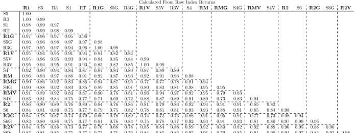
Accordingly, we compute across-group correlations between equal-weighted APB residuals from the four-factor regression. Under the null of uncorrelated (idiosyncratic) fund strategies across different groups, we expect to find correlations that are not significantly different from zero. To test this, we compute correlations between APB groups over the 30-year period from 1980 to 2009. To allow for unstable regression loadings over time, we compute, for each of the 10 non-overlapping three-year periods, the four-factor residuals for each APB. Then, we splice these residuals into a 30-year record for each APB. Finally, we compute a Pearson
correlation between the residuals of each pair of APB residual time-series.18
Panel A of Table 2 shows substantial evidence of across-group commonality in idiosyncratic risk-taking, as we can reject the null of no correlation between APB residuals quite frequently. Specifically, 35 out of 36 possible correlation pairs are positive and significant at the 5% (two-tailed) confidence level. Indeed, some of the correlations are extremely high. Especially dramatic are the residual correlations involving midcap
18For a given three-year period for a given APB group, we require at least five (no-load) mutual funds to each have at least
30 monthly returns during that period in order to have a reasonably diversified group return. Otherwise, we omit that three-year period from the 30-three-year record for that APB, and compute pairwise correlations involving that APB over the remaining residuals.
and/or smallcap fund groups as pairs. Of course, some of this comes from the overlap in the indexes, but some may also result from funds that do not neatly fit within one APB group.
In Panel B, we test whether these high correlations are due to the overlap in indexes (either through the same securities, or through different securities in similar industries), and/or to the potential inability of the four-factor model to price index returns precisely. Cremers, Petajisto, and Zitzewitz (CPZ; 2012) find evidence that common market indexes exhibit significant estimated four-factor model alphas, and interpret this evidence as the inability of the four-factor model of Fama and French (1993) and Carhart (1997) to properly price passive assets. To explain, the four-factor model uses equal-weighting of, for example, Small-High and Big-Small-High portfolios for the value (high book-to-market) portion of their HML (value minus growth) portfolio. This weighting scheme underweights large capitalization stocks in favor of small stocks, while
market indexes are generally capitalization-weighted.19 Panel B shows correlations between the “best-fit”
passive index return residuals, after regressing the index returns on the four-factor model.
The results show, in general, substantially different correlations between the index residuals (Panel B) and the fund APB residuals (Panel A). For example, funds in the Russell Midcap Growth and those in the Russell Midcap groups exhibit a correlation of 0.74 (panel A), while the residuals for the underlying indexes exhibit a much smaller correlation of 0.42 (panel B). The difference in correlations between panels A and B suggest that, while the indexes do indeed appear to exhibit unmodeled commonalities when using the four-factor model, as suggested by CPZ, there appears to be some unmodeled commonalities between APB groups as well, controlling for index commonalities.
These results suggest that we may need to include multiple APB “factors” as additions to the four-factor model for each mutual fund. Therefore, in our robustness tests in Section 4.6, we implement a multiple APB factor augmented model; as we shall see, this multiple APB model demonstrates some usefulness in picking active funds with superior out-of-sample performance. For our main results, however, we use more parsimonious single-APB augmented models, as this model performs somewhat better, out-of-sample, than the more complicated multiple-APB model (due to overfitting by the multiple model).
4.3. Correlation Between Individual Equity Fund Residuals
Next, we turn to evaluating the performance of the four-factor model at the individual fund level. If the four-factor model captures systematic variation in returns properly, then the individual fund residuals will exhibit commonalities with each other only due to their loading on similar idiosyncratic factors. For instance, during the 1990s, many growth funds overweighted technology and telecommunication stocks in common, whose residuals may not be fully captured by the four-factor model.
Table 3 presents the percentage of significantly positive and the percentage of significantly negative (at the 10% two-tailed confidence level) pairwise correlations between individual fund residuals from the
four-factor model (Equation 7), out of all possible pairwise correlations in the group (see rows labeled “4 Factor”). For example, during 1980-1982, the Russell 1000 APB group contains 45 funds which yield 990
(45×442 ) pairwise correlations of residuals, among which 45%, or 446, are significantly positively correlated,
and 4%, or 40, are significantly negatively correlated.
First, note that the percentage of significant positive correlations, using the four-factor model, is always higher than the percentage of significant negative correlations–and, usually it is much higher. Specifically, on average across groups and subperiods, 37% of fund pairs have (significantly) positively correlated residuals, while 5% have negatively correlated residuals (see the values for the 4 Factor model in the final column and final four rows in Table 3). In fact, the percentage of negatively correlated residuals is what we would expect from randomly occurring correlations–5% with a two-tailed critical value of 10%. Further, this negative and significant percentage is reasonably constant across time-periods and fund groups, and rarely exceeds 10%. Turning to the percentage of pairwise correlations that are positive and significant, we see that this percentage is rarely below 20%, and it is often above 30%. Other than a sharp rise in positively correlated residuals during the late stages of the internet boom and the period immediately afterward (1998-2000 and 2001-2003, respectively)–when funds likely commonly tilted heavily toward tech and telecom–there is no apparent time-trend to the correlations. Positive correlations of four-factor residuals are especially common in midcap funds and smallcap funds, indicating an especially high degree of cohesiveness in strategies in these groups. Overall, positive and significant correlations in all groups suggest significant commonalities in the investment strategies across funds that are not captured by the four-factor model.
To illustrate the impact of our approach, the table also shows similar correlation statistics, computed using individual fund residuals from the augmented model of Equation (8), where we add the APB residual to the four-factor model (see rows labeled “4 Factor + APB”). Note the large drop in the percentage of positive correlations that are significant with this model, relative to the four-factor model. Specifically, the average positive percentage drops from 37% to 13%, while the negative percentage increases from 5% to 16%. Interestingly, for almost all groups and time-periods, the fraction of significant correlations is reasonably balanced between positive and negative values. Especially noteworthy is that the spike in positive correlations noted above, during 1998-2003, are no longer present. Clearly, the addition of the APB successfully controls for a good deal of common idiosyncratic risk-taking by funds within groups.
To summarize, the results of Tables 2 and 3 present evidence that supports that (1) standard factors leave a significant degree of unexplained covariation among funds within a group and across groups, and (2) a significant part of this covariation within a group can be controlled by adding the APB to the four-factor
model.20 This provides strong support for the use of our augmented model of Equation (8).
20We also note that the above results support that the classification by “best-fit index” successfully (for the most part)
4.4. Alpha Estimation Diagnostics
In this section, we demonstrate the influence of active peer-group benchmarks on alpha estimation. First, we compare three models of equities: the traditional four-factor model (Equation (7)), the APB augmented models (Equations (8) and (9)), and (for comparison) the model with only the APB factor (Equation (10)). The use of the four-factor model and the baseline APB model will result in the same estimate of alpha, since the APB factor is mean-zero, by construction. However, the t-statistic of the alpha of funds may increase (in absolute value) with the APB augmented model, if the APB factor adequately captures commonality in idiosyncratic risk-taking. On the contrary, the alpha-adjusted version of the augmented model (Equation (9)) and the APB-only model (Equation (10)) will result in different alpha estimates, since they are based on a different set of (non-zero mean) factors than the first two models. If the APB factor adequately captures commonality in idiosyncratic risk-taking, away from the benchmark, then the alpha-adjusted model should tighten the distribution of estimated alphas around zero. Our goal in this section is the determine whether the addition of the APB results in a sharper separation of funds into those with positive and negative alphas, relative to the baseline four-factor model.
Columns four through seven of Table 4 show the percentage of funds (within each APB category) having statistically significant market (rmrf), small (smb), value (hml), and momentum (umd) exposures,
respec-tively, while column eight shows similar statistics for the APB factor coefficient,λ,from the model of either
Equation (8) or Equation (9). To compute these percentages, we count the number of significant p-values, which are those below 2.5% (to correspond to a two-tailed 95% confidence region), and divide by the to-tal number of funds within a particular APB category. Further, within each group (e.g., “Russell 1000”), the first and fourth rows indicate the percentage of funds with significantly positive and negative alphas, respectively, while the second and third rows indicate the percentage of funds with insignificant alphas in each category.
Note that the results for rmrf, smb, hml, and umd are consistent with what we should expect from using a “best fit” index to categorize funds. For example, the majority of Russell 1000 Growth funds have a negative (and, in most cases, significant) exposure to hml, while the majority of Russell 1000 Value funds have a positive exposure. Meanwhile, “core funds” within the Russell 1000 or Russell Midcap categories
have more balanced percentages of funds with statistically significant loadings on hml.21 Further, midcap
and smallcap funds are much more likely to have a positive loading on smb. In addition, the APB factor
coefficient, λ, is significantly positive for over half of funds in each peer-group category, and much higher
in midcap and smallcap categories (indicating that it is more helpful in capturing common idiosyncratic risk-taking in these groups).
21An anomaly is the Russell 2000 group. Here, funds tend to load significantly on hml, but this is chiefly due to the index
having a significant loading on hml. In addition, the Russell 2000 value group has a slightly lower loading on hml than the
Russell 2000 group, but this is likely due to the infrequency of Russell rebalancing the 2000 indices. Some value stocks,
Next, the first column of Table 4 shows the percentage of funds, within each group, having statistically
significant four-factor alphas (see the column labeled “α”), while the second and third columns (“αaug” and
“aaug”, respectively) show the percentage of funds having significant alphas using the models of Equations
(8) and (9). The reader should note that the level of alphas for the four-factor and the augmented model of Equation (8) are equal, but t-statistics will generally be different due to the addition of the zero-mean
active-peer benchmark to create the augmented model.22 However, the level of alphas with the
“APB-adjusted alpha model” of Equation (9) will be different from the four-factor model due to the addition of
both the peer-group alpha and the zero-mean APB factor. Our results for the APB factor coefficient, λ,
cited above, indicate that the Equation (8) model should move alpha t-statistics further from zero, relative to the four-factor model, while the Equation (9) model will shrink alpha t-statistics back toward zero.
The results for all peer-groups can be illustrated by those for the Russell 1000 peer-group. First, the four-factor model indicates that there may be some pre-expense skilled fund managers, as the 6.9% of alphas having a p-value lower than 2.5% is much higher than expected by random chance. Next, the
APB-augmented model alpha, αaug, is more precisely separated into significantly positive and negative funds,
relative to the four factor alpha,α, indicating that the APB is effective at capturing return variation that
is common to many of the Russell 1000 funds. Specifically, the frequency of positive and significant alphas increase from 6.9 to 9.4%, while the frequency of negative and significant alphas increase from 3.9 to 5.1%. Clearly, the APB-augmented model indicates that there are more alpha outliers, relative to the four-factor model, especially in the positive alpha tail.
When we focus on the APB-adjusted alpha model, aaug, we find that (as expected from the large
frequency of positive APB factor coefficients, λ, noted above) t-statistics are pushed closer to zero. The
result is 5.9 and 5.8% significant positive and negative values ofaaug, respectively. Thus, almost half of the
significant positive alphas from the APB-augmented model, 9.4%, can be traced to strategies that are used in common by Russell 1000 funds (since the remaining significant positive alphas account for 5.9% of the group).
Results among other peer-groups are similar, except for the notable fact that the APB factor is more useful, in general, for explaining common variation in returns among midcap and smallcap funds, relative
to largecap funds (easily seen from comparing the percentage of positive and significant values of λ, the
coefficient on the APB factor). This result can be attributed to the large number of investable stocks within midcap and smallcap ranges, in addition to the apparent use of similar strategies by funds within these large choice sets.
Finally, it is instructive to consider the power of the APB factor alone to explain fund returns, using the
22Estimated alphas are the same because the first-stage APB residuals are estimated over the same three-year period as the
second-stage fund regression, thus, the first-stage APB residuals are mean-zero in both the first and second stage regressions, and do not affect the level of estimated fund alpha.
model of Equation (10). In column nine, we see that this single-factor model performs quite well, achieving
an adjusted R2 above 75% for all peer-group categories. For comparison, the adjusted R2 using the
four-factor model is generally only a few percent higher. This result indicates that our categorization of funds is successful, as it reflects that exposures to risk-factors as well as idiosyncratic risk have strong commonalities
within peer-groups.23
To summarize the results of this section, a significant percentage of funds appear to have both significantly positive and significantly negative alphas, using the APB-augmented model. However, a good deal of these funds lose their significant alphas when we control for the alphas earned by the common strategy (using the alpha-adjustment model). Indeed, among most peer-groups, the fraction of positive and significant alphas decrease, while the fraction of negative and significant alphas increase, indicating that common strategy alphas (controlled by the alpha-adjustment model) are generally positive. This result brings the possibility that we may capture superior alphas through a passive strategy of investing in an entire group of funds, rather than attempting to choose the best of the peer-group. Thus, a remaining important question is whether the above-noted alphas persist, and, if so, whether they are due to common strategies among a peer-group of funds or to idiosyncratic strategies of only a few funds in a peer-group.
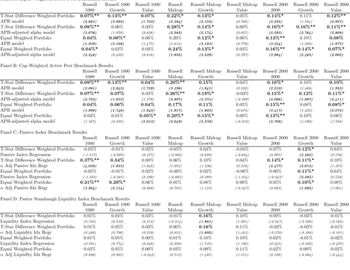
4.5. Out-of-Sample Performance 4.5.1. Pre-Expense Alpha
Does our APB model improve the identification of skilled fund managers? And, if so, do these skilled managers use common strategies as a subgroup of a peer-group, or do they use strategies that are distinct from each other? Our out-of-sample tests are designed to determine the answers to these questions. First, in untabulated tests, we find a relatively high rank correlation between t-statistics of fund alphas estimated from models with and without the endogenous factor. Thus, we would expect that out-of-sample performance differences between these models will be small. However, it is possible that the small differences can be exploited to increase the persistence in alphas from a fund selection strategy if there exist a minority of funds with superior skills.
We first explore the persistence in alphas for funds ranked on the t-statistic for their trailing three-year APB-augmented four-factor model alpha (Equation (8)). If the addition of the APB factor sufficiently adjusts for common idiosyncratic risk-taking, then the t-statistic of alpha should be an improved indicator of manager skills.
First, we conduct a very simple test of performance persistence, using our APB-augmented model of Equation (8). At the end of each month, starting on December 31, 1982 and ending on December 31, 2009, we rank all U.S. equity mutual funds by the t-statistic of alpha from that model, measured over the prior
23It is also notable that the peer-group factor, by construction, represents a tradable group of no-load funds, while trading
36 months (we require at least 30 months of returns to be non-missing during this period).24 Then, quartile
portfolios of funds are formed, and equal-weighted portfolio returns are computed over the following (out-of-sample) year. Next, we compute the alpha from Equation (8) over this year. Next, we move forward one month, and repeat this process. Finally, we compute time-series average alphas and time-series t-statistics of these alphas over all such (overlapping) out-of-sample years (with standard errors adjusted for the time-series overlapping nature of the windows over which the alphas are computed).
Panel A of Table 5 presents results from this exercise. The table shows that, in general, (pre-expense) alphas are monotonically decreasing from quartile 1 (top ranked funds from the prior three years) to quartile 4 (bottom ranked funds). For instance, in the Russell 1000 peer group, we find that top-quartile funds exhibit a
monthlyfour-factor model alpha of 7 bps (84 bps/year), while the second-, third-, and fourth-quartiles exhibit
alphas of 4, 4, and 0 bps, respectively. Among our nine peer-groups, we find that four exhibit significantly positive four-factor alphas for top-quartile funds, ranked by the APB-augmented model, while, in eight of nine groups, top-quartile funds significantly outperform bottom-quartile funds during the following year. And, no peer-groups exhibit negative alphas for top-quartile funds during the year following the ranking date.
It is also instructive to note the differences in the persistence of performance across different peer groups. Positive performance persistence (statistically significant 1st-quartile performance during the following year)
is especially strong among midcap funds, but is also present among largecap funds. Among smallcap
funds, the difference in alphas between 1st and 4th quartiles are especially pronounced, since persistence in underperformance is present in these groups of funds. Since these alphas are gross of fees, but net of trading costs, the absence of stock-selection skills among smallcap funds is especially costly–since trading costs are a significant drag on smallcap fund performance.
In Panel B, we conduct the same ranking and portfolio formation procedures, but we measure the following-year performance with the redefined alpha from the alpha-adjustment model of Equation (9). If our 1st quartile funds manage to outperform simply due to the (leveraged) use of strategies common to the peer group, then the inclusion of the peer group alpha (leveraged by the fund’s exposure to the peer group
factor) will result in an insignificant residual alpha (ai from Equation (9)). However, the results indicate
that top-quartile funds exhibit significant persistence in 6 of 9 peer groups. Among largecap and midcap peer groups, the alpha is reduced from its value in Panel A, but, among smallcap groups, the alpha actually increases. This observation reflects that the common strategies of largecap and midcap funds produce persistent and positive alphas, but those of smallcap funds produce somewhat negative alphas. The overall results indicate evidence of skills among several fund groups–large, mid, and small–but indicate that skilled smallcap fund managers perform better when they deviate from the group. Largecap and midcap managers
24Note that we rank by alpha t-statistic, since the advantage of our APB-augmented model is reflected in this parameter. In