An Option Pricing Formula for the GARCH Diffusion Model
∗Giovanni Barone-Adesia, Henrik Rasmussenb and Claudia Ravanellia First Version: January 2003
Revised: September 2003
Abstract
We derive analytically the first four conditional moments of the integrated variance implied by the GARCH diffusion process. From these moments we obtain an analytical closed-form approximation formula to price European options under the GARCH diffusion model. Using Monte Carlo simulations, we show that this approximation formula is accurate for a large set of reasonable parameters. Finally, we use the closed-form option pricing solution to shed light on the qualitative properties of implied volatility surfaces induced by GARCH diffusion models.
aInstitute of Finance, University of Southern Switzerland, Lugano, CH. bMathematical Institute, University of Oxford, Oxford, UK.
∗Corresponding author: Claudia Ravanelli, University of Southern Switzerland, Institute of Finance, Via
Buffi 13, CH-6900, Lugano, tel: +41 (0)91 912 47 86. E-mail: [email protected]. Giovanni Barone-Adesi and Claudia Ravanelli gratefully acknowledge the financial support of the Swiss National Science Foundation and NCCR FINRISK. The authors thank Jerome Detemple and Loriano Mancini for their valuable suggestions.
1
Introduction
In this paper we study European option prices in stochastic volatility models where the underly-ing asset follows a geometric Brownian motion with instantaneous variance driven by a GARCH diffusion process. Precisely, we derive analytically a closed-form approximation for European option prices under the GARCH diffusion model.
Stochastic volatility models were first introduced by Hull and White (1987), Scott (1987) and Wiggins (1987) to overcome the drawbacks of the Black and Scholes (1973) and Merton (1973) model. Volatilities, stochastically changing over time, account for random behaviours of im-plied and historical variances and generate some of the log-return features observed in empirical studies1. Unfortunately, in the stochastic volatility setting it is difficult to derive closed or ana-lytically tractable option pricing formulas even for European options. The Hull and White (1987) and the Heston (1993) models have an analytical approximation and a quasi-analytical formula to price European options, respectively. For other stochastic volatility models numerical meth-ods are available but these procedures are highly computationally intensive2. In this paper, we derive an analytical closed-form approximation for European option prices based on the con-ditional moments of the integrated variance when the variance is driven by an uncorrelated GARCH diffusion process3. Our approximation is very accurate and easy to implement, it can be used to study the implied volatility and the volatility risk premium associated to GARCH diffusion models.
The GARCH diffusion process has several desirable properties. It is positive, mean reverting, with a stationary inverse Gamma distribution and it satisfies the restriction that both historical and implied variances be positive. It also fits the observation that variances seem to be station-ary and mean reverting; cf. Scott (1987), Taylor (1994), Jorion (1995) and Guo (1996, 1998). Moreover, the GARCH diffusion model allows for rich pattern behaviours of volatilities and asset prices. For instance, as observed in empirical studies, it produces large autocorrelation in the squared log-returns, arbitrary large kurtosis and finite unconditional moments of log-return distributions up to a given order. By contrast, when the variance follows a square root process as in the Heston (1993) model the corresponding stationary Gamma distribution implies log-return distributions with finite unconditional moments of any order and not very large kurtosis4; cf.
1See , for instance, Mandelbrot (1963) and Fama (1965).
2When large trading books have to be quickly and frequently evaluated many procedures are practically not
feasible.
3This model was first introduced by Wong (1964) and popularized by Nelson (1990).
4Rejections of the Heston model are reported by several authors, see for instance Andersen et al. (2002),
Genon-Catalot, Jeantheau and Laredo (2000).
Furthermore, Nelson (1990) showed that under the GARCH diffusion model discrete time log-returns follow a GARCH(1,1) in mean ((GARCH(1,1)-M) process of Engle and Boller-slev (1986)). Hence, the nasty problem of making inference on continuous time parameters may be reduced to the inference on the GARCH(1,1)-M model; cf., for instance, Engle and Lee (1996) and Lewis (2000). This is an important advantage over other stochastic volatility models which lack of these simple estimators. In a Monte Carlo study we investigate inference results based on such an estimation procedure. Finally, the GARCH diffusion model is the ‘mean reverting’ extension of the Hull and White (1987) model where the variance process follows an uncorrelated log-normal process without drift. The GARCH diffusion model makes a marked improvement over the Hull and White model because the mean reverting drift gives stationary variance and log-return processes (cf. Genon-Catalot, Jeantheau and Laredo (2000)) and it can include the volatility risk premium in the variance process. By contrast, for the Hull and White model the analytical option pricing approximation is available only when the drift is equal to zero5. Furthermore, the mean reversion of the variance allows to approximate long maturity option prices, while in the Hull and White model the option pricing approximation holds only for short maturity options; cf. Hull and White (1987) and Gesser and Poncet (1997).
Our approximation for option prices under the GARCH diffusion model is based on the Hull and White (1987) formula, which holds when the asset price and the instantaneous variance are uncorrelated. This assumption implies symmetric volatility ‘smiles’, i.e. symmetric shapes of implied volatilities plotted versus strike prices; cf. Hull and White (1987) and Renault and Touzi (1996). Typically, foreign currency option markets are characterized by symmetric volatil-ity smiles; cf., for instance, Chesney and Scott (1989), Melino and Turbull (1990), Taylor and Xu (1994) and Bollerslev and Zhou (2002). Therefore, the present model can be appropriate to price currency options. Furthermore, also in some index option markets the non zero correlation between price and variance can be neglected without increasing option pricing errors; cf. Cher-nov and Ghysels (2000) and Jones (2003) for studies on Standard & Poor’s 500 and Standard & Poor’s 100, respectively.
The specific contributions of this paper are the following. We derive analytically the first four conditional moments of the integrated variance implied by the GARCH diffusion process. This result has several important implications. Firstly and foremost, these conditional moments of Heston is incapable of generating realistic [index] returns behaviour, and data are better represented by a stochastic variance model in the CEV class” as the GARCH diffusion model.
5The volatility risk premium seems to be a significant component of the risk premia in many currency markets;
allow to obtain an analytical closed-form approximation for European option prices under the GARCH diffusion model. This approximation can be easily implemented in any software pack-age (such as Excel spread sheets). Then, just plugging in the model parameters, it provides option prices without any computational efforts. As we will show by Monte Carlo simulations, this approximation is very accurate across different strikes and maturities for a large set of rea-sonable parameters. Secondly, we propose an analytical approximation for implied volatilities based on the conditional moments of the integrated variance, which allows us to easily study volatility surfaces induced by GARCH diffusion models. Thirdly, the conditional moments of the integrated variance implied by the GARCH diffusion process generalize the conditional moments derived by Hull and White (1987) for log-normal variance processes. Finally, the conditional moments of the integrated variance can be used to estimate the continuous time parameters of the GARCH diffusion model using high frequency data6. As already mentioned, Nelson’s theory suggest an appealing estimation procedure for the GARCH diffusion model parameters. By Monte Carlo simulation we investigate the accuracy of such inference results.
The rest of the paper is organized as follows. Section 2 introduces the GARCH diffusion model. Section 3 presents the analytical approximation formula to price European vanilla options under the GARCH diffusion model. In Section 4, using Monte Carlo simulations, the accuracy of the approximation is investigated across different strike prices and time to maturities for different parameter choices. Section 5 studies implied volatility surfaces induced by the model. Section 6 studies the accuracy of the inference on the GARCH diffusion model based on the Nelson’s theory and Section 7 concludes.
2
The Model
Let S = (St)t≥0 be the underlying currency price and V = (Vt)t≥0 its latent instantaneous variance. We assume that (St, Vt)t≥0 satisfies the two-dimensional GARCH diffusion model
dSt=µ Stdt+ p
VtStdBt, (1)
dVt= (c1−c2Vt)dt+c3VtdWt, (2)
wherec1, c2 and c3 are positive constants,µis the positive constant drift of dSt/St, B and W are mutually independent one-dimensional Brownian motions on some filtered probability space (Ω,F,Ft,P) andPis the objective measure. We set the initial timet= 0 and (S0, V0)∈R+×R+.
6By matching the sample moments of the realized volatility with the conditional moments of the integrated
variance one has a standard and easy to compute GMM-type estimator for the underlying model parameters; cf. Bollerslev and Zhou (2002).
TheV process is mean reverting,c1/c2 determines the run mean value andc2 is the reversion rate (see also equation (4)). For ‘small’ c2 the mean reversion is ‘weak’ and Vt tends to stay above (or below) the run mean value for long periods, i.e. to volatility cluster. The parameter c3 determines the random behaviour of the volatility: forc3 = 0 the volatility process is deter-ministic, for c3 >0 the kurtosis of log-return distributions is larger than 3. When c1 =c2 = 0, the GARCH diffusion process reduces to the log-normal process without drift in the Hull and White (1987) model.
Given V0 >0,Vt is positiveP-almost surely∀t≥0, and the strong solution is
Vt=V0 e−(c2+ 1 2c23)t+c3Wt + c 1 Z t 0 e(c2+12c23)(s−t) +c3(Wt−Ws)ds, (3)
see Karatzas and Shreve (1991), p. 360. The stationary distribution ofV is the Inverse Gamma distribution (cf. Nelson (1990)) with parameters 1 + 2c2/c23 and c32/2c1, i.e. 1/Vt ; Γ(1 + 2c2/c2
3, c23/2c1). Hence Vt has finite moments up to order r if and only if r < 1 + 2c2/c23. This implies that log-return distributions have finite unconditional moments up to order 2r. Empirical studies showed that log-return distributions have finite moments up to some given order. Moreover, when c2
3 →2c+2, the kurtosis of log-return distributions tends to infinity and the correlation between squared log-returns approaches to 1/3.
When 2c2 > c23, the V process is strictly stationary, ergodic with conditional mean and variance E[Vt|V0] = cc1 2 + (V0− c1 c2)e −c2t, (4) Var[Vt|V0] = (c1/c2) 2 2c2/c23−1 + e−c2t2(c1/c2)(V0−(c1/c2)) c2/c23−1 − e−2c2t (V 0−(c1/c2))2 +e(c23−2c2)t µ V02−2V0(c1/c2) 1−c2 3/c2 + (c1/c2)2 (1−c2 3/2c2)(1−c23/c2) ¶ . (5)
The unconditional expectation of (4) and (5) give the unconditional mean and variance of V
E[V1] = cc1 2, Var[V1] = (c1/c2)2 2c2/c2 3−1 . (6)
In Section 4 we will infer some reasonable parameters for the variance process using equations (6). Higher order unconditional moments of V can be derived by the stationary Inverse Gamma distribution.
In the following section we will derive an analytical approximation formula for European options when the underlying currency price satisfies equations (1)–(2).
3
The Option Pricing Formula
Given the model (1)–(2), a foreign currency option pricef(S, V, t) satisfies the following partial differential equation 1 2V S 2 ∂f2 ∂S2+ 1 2c 2 3V2 ∂f2 ∂V2+(rd−rf)S ∂f ∂S+((c1−c2)V−λ(S, V, t)) ∂f ∂V −(rd−rf)f+ ∂f ∂t = 0, whererdandrf are the domestic and the foreign interest rates, respectively, and the unspecified term λ(S, V, t) represents the market price of risk associated to the variance V. As in other studies (see, for instance, Chesney and Scott (1989), Heston (1993) and Jones (2003)), we specify the volatility risk premium as λ(V, S, t) =λV. The risk-adjusted process still remains a GARCH diffusion process,
dSt= (rd−rf)Stdt+ p
VtStdB∗t, (7)
dVt= (c1−c∗2Vt)dt+c3VtdWt∗, (8)
where c∗
2 = c2 +λ, B∗ and W∗ are mutually independent Brownian motions under the risk-adjusted measure P∗.
For the risk-adjusted dynamics in equations (7)–(8) the option pricing result in Hull and White (1987) holds: the fair price valueCsv for a European call with time to maturity T and strike priceK is given by
Csv = Z ∞
0
Cbs(VT)f(VT |V0)dVT, (9)
whereCbs is the Black and Scholes (1973) option price, VT is the integrated variance over the time to maturityT, i.e.
VT := T1 Z T
0
Vtdt (10)
and f(VT | V0) is the conditional density function of VT given V0. The integrated variance density f(VT |V0) is not known and the option price Csv is not available in closed-form. The expectation in equation (9) can be computed by Monte Carlo simulation but such a procedure is very time-consuming. Hull and White (1987) provided an analytical approximation forCsv in (9). Precisely, they computed the Taylor expansion ofCbsin equation (9) around the conditional mean ofVT obtaining a series option pricing formula that involves only the conditional moments of VT and the sensitivities of the Black and Scholes price to the variance. Denoting by M1 :=
E[VT |V0] the conditional mean ofVT and Mic :=E[(VT −M1)i |V0] i≥2 the i-th centered conditional moment ofVT, the option pricing series is
Csv =Cbs(M1)+12M2c ∂ 2C bs ∂V2T ¯ ¯ ¯ ¯ ¯ VT=M1 +1 6M3c ∂3C bs ∂V3T ¯ ¯ ¯ ¯ ¯ VT=M1 + 1 24M4c ∂4C bs ∂V4T ¯ ¯ ¯ ¯ ¯ VT=M1 +..., (11)
where the derivatives are ∂Cbs ∂VT = e−rfTS 0 √ T e−d21/2 p 8πVT , (12) ∂2C bs ∂V2T = ∂Cbs ∂VT · 1 2 m2 (VTT)2 − 1 2VTT − 1 8 ¸ T, ∂3C bs ∂V3T = ∂Cbs ∂VT · m4 4(VTT)4 −m2(12 +VTT) 8(VTT)3 +48 + 8VTT+ (VTT)2 64(VTT)2 ¸ T2, ∂4C bs ∂V4T = ∂Cbs ∂VT " 1 8 m6 (VTT)6 − 3 32 m4(20 +V TT) (VTT)5 + 3 128 m2(240 + 24V TT + (VTT)2) (VTT)4 −(960 + 144VTT+ 12(VTT) 2 + (VTT)3) 512(VTT)3 # T3,
and m := log(S0/K) + (rd−rf)T. So far, the conditional moments of the integrated variance have been calculated analytically only for few specifications of the variance process
1. for the mean reverting Ornstein-Uhlenbeck process7Cox and Miller (1972, Sec. 5.8) derived the first two conditional moments ofVT;
2. for the geometric Brownian motion with drift Hull and White (1987) derived the first two conditional moments ofVT and the first three conditional moments ofVT for the variance process without drift;
3. for the squared root process Bollerslev and Zhou (2002) derived the first two conditional moments. Lewis (2000a) derived the first four conditional moments of the integrated variance for the general class of affine processes (including the squared root process). Given the analytical conditional moments ofVT it is very easy to price European options by the series approximation (11). Garcia, Lewis and Renault (2001) use this formula to price European options under the Heston model notwithstanding the Heston option pricing formula; cf. also Ball and Roma (1994). Indeed, implementing integral solutions for option prices, such as the Heston formula, can be very delicate due to divergence of the integrand in some regions of the parameter space.
We derive the first four conditional moments of VT when the variance V is driven by the GARCH diffusion process (2). The first conditional moment is already known in the litera-ture. The second, the third and the fourth are believed to be new. Higher order moments are essential to capture the ‘smile’ effect of implied volatilities; cf., for instance, Bodurtha and
7We recall that the mean reverting Ornstein-Uhlenbeck process is normally distributed and then can not ensure
Courtadon (1987) for PHLX foreign currency options and Lewis (2000). We denote these con-ditional moments by M1gd, M2cgd, M3cgd and M4cgd. Here we stateM1gd, M2cgd and the calculations are given in Appendix A. The third and the fourth conditional moments are more involved and are available from the authors on request.
Proposition 3.1 Let V = (Vt)t≥0 to satisfy the stochastic differential equation (2). Given (V0, c1) ∈R+×R+ and c2 > c23, the first and the second conditional moment of the integrated varianceVT are M1gd :=E[VT|V0] = cc1 2 + (V0− c1 c2) 1−e−c2T c2T , (13) M2cgd :=E[(VT −M1gd) 2 |V0] =−e −2T c2(c 2V0−c1)2 T2c4 2 +2e(c 2 3−2c2)T (2c2 1+ 2c1(c23−2c2)V0+ (2c22−3c2c23+c43)V02) T2(c2−c2 3)2(2c2−c23)2 −c23(c21(4c2(3−T c2) + (2T c2−5)c23) + 2c1c2(−2c2+c23)V0+c22(−2c2+c23)V02) T2c4 2(−2c2+c23)2 +2e−T c2c23(2c21(T c22−(1 +T c2)c23) + 2c1c22(1−T c2+T c23)V0+c22(c23−c2)V02) T2c4 2(c2−c23)2 . (14) These moments are obtained using properties of Brownian motion such as independence and stationarity of non-overlapping increments and the linearity of dVt inVt. As already observed, forc1 = 0 the GARCH diffusion process reduces to the log-normal process with drift and then M1gd,M2cgd reduce to the conditional mean and variance ofVT in Hull and White (1987), p. 287. Given the first four conditional moments ofVT, under the GARCH diffusion model the call price is e Cgd =Cbs(M1gd) +1 2M gd 2c ∂2C bs ∂V2T ¯ ¯ ¯ ¯ ¯ VT=M1gd +1 6M gd 3c ∂3C bs ∂V3T ¯ ¯ ¯ ¯ ¯ VT=M1gd + 1 24M gd 4c ∂4C bs ∂V4T ¯ ¯ ¯ ¯ ¯ VT=M1gd . (15) AlthoughM1gd,M2cgd,M3cgdandM4cgdare rather nasty, the closed-form approximation formula (15) can be easily implemented in any software package (such as Excel spread sheets) providing option prices by just plugging in model parameters without any computational efforts.
As we will show in the next section, our approximation formula (15) is very accurate for a large set of reasonable parameters. Intuitively, when the time to maturity T is ‘short’, VT is not too far fromM1gd := E[VT|V0], then we expect approximation (15) to converge quickly.
When the time to maturityT increases,M1gd tends to the run mean value of V,E[M1gd] =c1/c2, and M2c, M3c and M4c go to zero. Therefore, we expect the approximation formula (15) to work well also for long maturities. By contrast, in the Hull and White (1987) model, where the variance Vt follows a log-normal process without drift, M2c and M3c tend to infinity when T increases and the series (11) fails to give the right price; cf. Hull and White (1987) and Gesser and Poncet (1997). The effect of moving to a mean reverting process from a log-normal process is to avoid that the variance explodes or goes to zero whenT increases.
Lewis (2000) derived a closed-form approximation for European option prices for a large class of stochastic volatility models including the GARCH diffusion model (7)–(8). Lewis’s approximation formula for European option prices is based on second order Taylor expansion of some complex integrals around c3 = 0; see Lewis (2000), p. 77–84. When c3 = 0, VT is deterministic and equals to M1gd. Indeed, it can be shown that Lewis’s approximation is a particular case of our approximation (15) and is obtained by (15) neglecting terms o(c2
3). Therefore, for the GARCH diffusion model, our approximation is more accurate than the Lewis’s one.
In the following section, by Monte Carlo simulations we study the accuracy of the approxi-mation formula (15).
4
Monte Carlo Simulations
In order to verify the accuracy of the approximation (15) we compute by Monte Carlo simulations European option prices. The advantage of using Monte Carlo estimates is that the standard error of estimates is known. Precisely, we compute put option prices8 implied by (9) using the conditional Monte Carlo method; cf. Boyle, Broadie and Glasserman (1997).
Specifically, we divide the time interval [0, T] intosequal subintervals and we draws indepen-dent standard normal variables (υi)i=1,...,s. We simulate the random variable Vtin (8) over the discrete timeiT /s, fori= 1, . . . , s, using the Milstein scheme (cf. Kloeden and Platen (1999))
Vi =c1∆t+Vi−1(1−c∗2∆t+c3√∆t υi) +1 2c 2 3Vi2−1(( √ ∆t υi)2−∆t),
where ∆t:=T /s. Then, we compute the Black and Scholes put option pricePbs(n) with squared volatility s−1Psi=1Vi. Finally, iterating this procedure N times we obtain the Monte Carlo
8Monte Carlo standard errors are generally smaller for put option prices than for call option prices as in the
estimate for the put option price Pmc:=N−1 N X n=1 Pbs(n),
with the corresponding Monte Carlo standard error emc:=
q
N−1PN
n=1√(Pbs(n)−Pmc)2
N .
When N goes to infinity, Pmc converges in probability to the put option price implied by (9). Notice that we do not need to simulate the price processS.
To simulate the variance process (8) we use parameter values inferred from empirical esti-mates of model (7)–(8). Typically, for currency and index daily log-returns the unconditional mean of V, c1/c∗2, ranges from 0.01 to 0.1 per year. The ‘half life’9 varies from few days to about a half year; cf. Chesney and Scott (1989), Taylor and Xu (1994), Xu and Taylor (1994), Guo (1996, 1998) and Fouque, Papanicolaou and Sircar (2000). This implies that c∗
2 ranges from 1 to 40. Moreover, empirical estimates of discrete GARCH(1,1)-M model on currency and index daily log-returns imply values ofc3 ranging from about 1 to 4; cf., for instance, Hull and White (1987a, 1988) and Guo (1996,1998). For stock log-returns, estimates ofc3 are generally smaller.
For the Monte Carlo simulations, we consider time to maturities for European put options ranging from 30 to 504 days. We wrote a Matlab code to run N = 106 simulations. The computation time goes from about 14 hours forT = 30 days to 15 hours forT = 504 days on a PC Pentium IV 1GHz, running Windows XP.
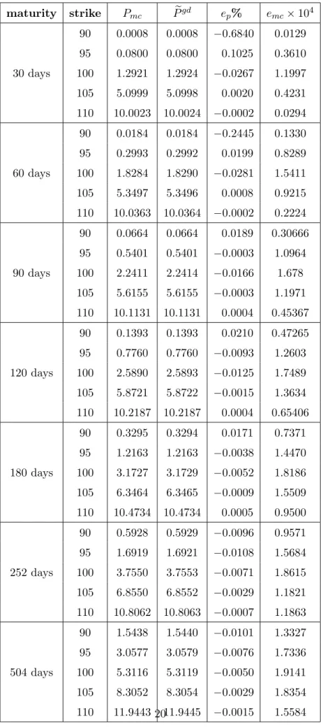
In Table 1 we simulate the risk-adjusted variance process (8) using parameter values that we infer (cf. Nelson (1990)) from the GARCH(1,1) estimates in Guo (1996) for the dollar/yen exchange rates10, i.e. c
1 = 0.16, c∗2 = 18 and c3 = 1.8. The variance process is quickly mean reverting (the half life is about 10 days) and rather volatile, the two-standard deviation range for V is from 0.003 to 0.016; see equations (6). Table 1 shows the Monte Carlo put price Pmc, the put price Pegd given by the series approximation (15), the pricing error ep% defined as ep% := 100×(Pmc−Pegd)/Pmc and the Monte Carlo standard error emc. All errors are practically negligible across all strikes and maturities and the average error is −0.025%. Although the variance process is rather volatile, the high mean reversion rate c∗
2 implies that the integrated variance processVT tends to stay around E[VT|V0] and then the approximation (15) works well.
9The ‘half life’ is the time necessary after a shock to halve the deviation ofV
t from its run mean value, given
that there are no more shocks. For this model the half life is equal to ln (2)/c∗
2 years. 10As in Guo (1996) we assume the volatility risk premiumλ(S, V, t) = 0.
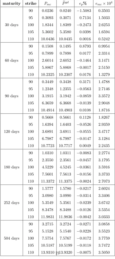
In Table 2 we simulate the variance process (8) using the risk-neutral parameters estimated by Melenberg and Werker (2001) for the Dutch EOE index. The volatility risk premium was estimated using European call options on the Dutch index. The correlation between price and volatility was negligible. The risk-neutral coefficients are c1 = 0.53, c2∗ = 29.23 andc3 = 3.65. The run mean value of the variance is 0.018 and the two-standard deviation range for V is 0–0.03. Table 2 is organized as Table 1. Also in this case pricing errors ep% are almost always lower than 1% (except for one case). The average error is−0.011%.
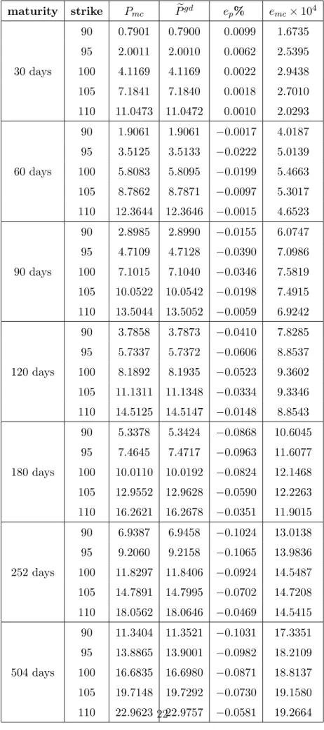
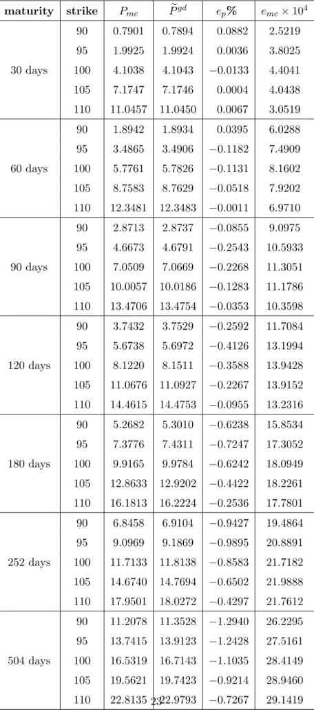
In Table 3 and Table 4 we use parameter values that give reasonable variance process as discussed in Hull and White (1988). In Table 3 we set c1 = 0.18, c∗2 = 2 and c3 = 0.8. The parameter valuec∗2 is quite small and implies a ‘slow’ mean reverting variance process (8), the half life of about 88 days. The unconditional mean and standard deviation of V are 0.09 and 0.03, respectively, and the two-standard deviation range for V is 0.01–0.16. As the volatility of Vt is not too large, the process VT tends to stay around E[VT|V0] and hence the series approximation (15) is very accurate. The average pricing error is −0.044%. In Table 4 we set c1 and c∗2 as in Table 3 and c3 = 1.2. This implies that the standard deviation of V is 0.06 and the two-standard deviation range for V is 0–0.22. Table 4 shows that pricing errors ep% are still very small (the average pricing error is −0.2%) but slightly larger than in Table 3 as the variance process is more volatile than in the previous case.
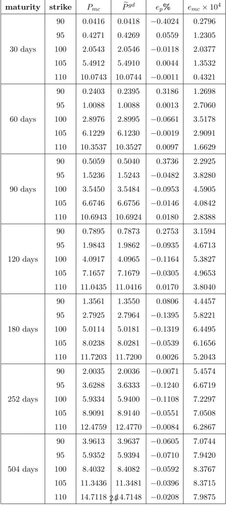
Finally, in Table 5 we setc1= 0.09,c∗2 = 4 andc3= 1.2 as in Lewis (2000). The unconditional mean ofV is 0.02, the ‘half life’ is about 43 days and the two-standard deviation range forV is 0.001–0.04. Also in this case errorsep% are generally quite small and the average pricing error is−0.018%.
We simulate the variance process (8) also for other reasonable parameter choices (not re-ported here) and we found similar results. The approximation formula (15) induces pricing errors less than 1% for at the money options and less than 2% for out of the money options. Bid-ask spreads on currency option prices are larger than 2% of the prices for out of the money options and about 1% for more liquid, at the money currency options. Then, the approximation formula (15) gives accurate prices within the tolerance imposed by market frictions.
5
Implied Volatility Surfaces
In this section we study the implied volatility induced by the GARCH diffusion model (7)–(8), i.e. the volatilityσ2
impwhich gives the Black and Scholes option price equals to the GARCH diffusion option price, Cbs(σimp2 ) = Cegd. Typically, to solve the implicit equation Cbs(σ2imp) = Cegd the
Newton-Raphson method is used11. Hence, we propose to computeσ2imp as σimp2 =M1gd+ Ce gd−C bs(M1gd) ∂Cbs/∂VT¯¯V T=M1gd , (16)
that is a one-step Newton-Raphson algorithm starting atM1gd. As σ2
imp→M1gd when T → ∞, M1gd is a sensible starting point for the algorithm and one iteration gives very accurate results12. GivenCegd implementing (16) is straightforward and the model (7)–(8) can be easily calibrated to the market implied volatilities.
Renault and Touzi (1996) show that, forany stochastic volatility process, the assumption of no correlation between price and variance induces symmetric ‘volatility smiles’, i.e. symmetric shape with respect to the forward price of the implied volatility plotted as a function of the strike price; cf. also Hull and White (1987). The functional dependence of implied volatilities on time to maturities, i.e. the ‘term structure patterns’, depends on the specific variance process. In the following we qualitatively study the volatility smile and the term structure pattern induced by the GARCH diffusion model. As in Table 5 we set c1 = 0.09, c∗
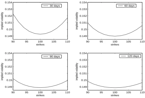
2 = 4 and c3 = 1.2 and we compute the GARCH diffusion option prices (15). Then, by formula (16) we obtain the implied volatilities for different strikes and maturities. Figure 1 shows volatility smiles for time to maturities equal to 30, 60, 90 and 120 days. Figure 2 shows the volatility surface for time to maturity between 0 and 120 days and strike prices between 90 and 110. As expected, volatility smiles are quite symmetric with respect to the forward price. Moreover, the convexity of the volatility surface increases when the time to maturity decreases. These features of implied volatility surface were observed for all parameter choices (positive parameters). When the time to maturity increases the volatility surface flattens because the random variable VT converges to the the run mean value c∗
1/c∗2 by the Ergodic theorem andσimp2 → c∗1/c∗2 for all strike prices. These results are in qualitative agreement with the empirical evidence on volatility surfaces observed in currency option markets, where volatility smiles are quite symmetric with respect to the forward price, very pronounced at short maturities and almost flat for long maturities; cf., for instance, Chesney and Scott (1989), Melino and Turbull (1990), Taylor and Xu (1994), and Bollerslev and Zhou (2002).
11See for instance the Matlab functionblsimpvdivand the Mathematica functionBlackScholesCallImpVol. 12We compared implied volatilities given by (16) with implied volatilities returned by the Matlab function
6
Simple Estimators based on Nelson’s Theory
Inference on continuous time parameters of stochastic volatility models is an important issue in financial econometrics. The intractable likelihood functions and the unobservable volatility pro-cess prevent simple and efficient estimation procedures13. Nelson (1990) derived some moment conditions under which the discrete time GARCH(1,1)-M model (cf. Engle and Bollerslev 1986)) converges in distribution to the GARCH diffusion model (1)–(2). Such a convergence has been advocated by many authors (see, for instance, Engle and Lee (1996) and Lewis (2000)) to infer the continuous time parameters by the parameter estimates of the GARCH(1,1)-M model. As such models can be easily estimated, the previous inference procedures is very appealing. How-ever, to our knowledge, the accuracy of the continuous time parameter estimates obtained by the discrete time parameter estimates have not been adequately verified.
In this section we investigate by Monte Carlo simulation how Nelson’s theory works in practice and the convergence, under previous conditions, of the stochastic difference equations (17) to the stochastic differential equations (1)–(2) whenh, i.e. the length of the discrete time interval between two observations, goes to zero.
The discrete time GARCH(1,1)-M model is Ykh = Y(k−1)h+ [µ−0.5σ2
kh]h+σkhZkh σ2
(k+1)h = w(h)+β(h)σ2kh+α(h)σ2khZkh2 h−1,
(17) where Ykh := log(Skh),, k ∈ N, Zkh ∼ i.i.d.N(0, h) and σ2
kh is the conditional variance of Ykh −Y(k−1)h. Using a moment matching procedure Nelson showed that, when h ↓ 0, the sequence of continuous time version of (17) converges in distribution to the continuous time process (1)–(2). Nelson’s procedure also yields the following relation between continuos and discrete time parameters up to o(h),
c1=w(h)/h, c2 = 1−β(h)−α(h), c3 =α(h) p
2/h, (18)
cf. Nelson (1990), pp. 15–18. Then, simple Maximum Likelihood estimates of model (17) allow to infer c1, c2 and c3. Moreover, as h shrinks the inference results should be more accurate. Using an Euler scheme14, we simulate 1,000 sample path realizations of the GARCH diffusion
13Several estimation methods have been proposed, such as the simulation based method of moments (Duffie
and Singleton (1993)) or Bayesian Markov chain Monte Carlo methods (Jones (2003)). Surveys on stochastic volatility models including the estimation problem are given by, for instance, Bollerslev et al. (1994) and Ghysels et al. (1996).
14The Euler scheme for equations (1)–(2) used here is log(S
i) = log(Si−1) + [µ−0.5Vi−1]∆t+
√
Vi−1∆t ²i
and Vi = c1∆t+Vi−1[1−c2∆t+c3
√
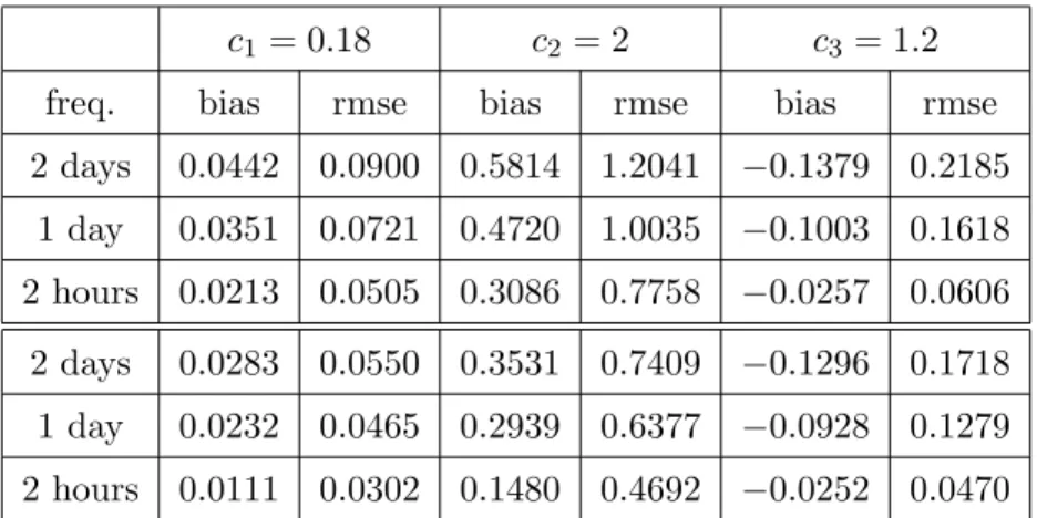
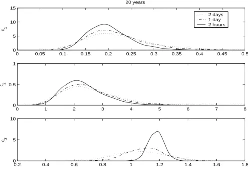
process (St, Vt)t∈[0,Tsmp], for the parameter choice c1 = 0.18, c2 = 2, c3 = 1.2 (as in Table 4) and Tsmp = 20, 40 years. For each sample path, we estimate the model (17) using two-daily (h = 2/360), daily (h = 1/360) and two-hourly (h = 1/3,000) log-returns and then we infer the continuous time parameters by formulae (18). The estimation results are given in Table 6 and Figure 3 and 4. As predicted by Nelson’s theory, higher the sampling frequency more accurate the inference results are in terms of biases and root mean square errors. Obviously, results based on Tsmp = 40 years are more accurate, but such a sample size is unrealistic for empirical studies. This simple and parsimonious estimation procedure provides still accurate inference results using Tsmp = 20 years of simulated data. Other continuous time parameters lead to similar results. Hence, such a procedure may be used for inference on GARCH diffusion model parameters. More involved estimation procedures should be required to outperform the above results. Finally, when Tsmp = 40 years, for two-daily estimates the sample size is large enough to overcome finite sample problems and regard the estimates as asymptotic15.
7
Conclusions
We derive analytically the first four conditional moments of the integrated variance under the GARCH diffusion model. Using these conditional moments we obtain an analytical closed-form approximation closed-formula Cegd (15) which allows us to price European options under the GARCH diffusion model. This formula can be easily implemented in any software package and provides option prices without any computational efforts. Monte Carlo simulations show that this approximation is accurate across different strikes and maturities for a large set of reasonable parameters. Finally, using the approximation formula (15) we study implied volatility surfaces induced by GARCH diffusion models. We find that volatility smiles and term structure patterns of implied volatilities are in qualitative agreement with volatility surfaces typically observed in the foreign exchange option markets.
Finally, we briefly investigate the inference on GARCH diffusion model parameters using an estimator based on Nelson’s theory. We conclude that, considering the simple and parsimonious estimation procedure, inference results are rather accurate. Hence, this procedure may be used to infer GARCH diffusion model parameters.
variables and ∆t= 1/(360×24). The sample path approximation to the diffusion can be made arbitrarily close by increasing the number of equally spaced increments per unit time interval. In this setting, the Milstein scheme is not advisable as multiple stochastic integrals can not be easily expressed in terms of increments of Brownian Motions; see for instance Kloeden and Platen (1999).
15We repeat the Monte Carlo study usingT
A
Proof of Proposition 3.1
In the following, we derive the first two conditional moments of the integrated varianceVT for the GARCH diffusion process,
VT = VT0 Z T 0 dt e−(c2+12c23)tec3Wt+ c1 T Z T 0 dt Z t 0 ds e(c2+12c23)(s−t)ec3(Wt−Ws). (19)
To prove Proposition 3.1 we recall that, ifw is a normal random variablew∼ N(0, t)
E[eλw] =eλ22t. (20)
We also need the following lemma
Lemma A.1 ∀ x > y >0, F(x, y) =e−(c2+12c23)(x+y)E[ec3(Wx+Wy)] =e−c2xe(c23−c2)y. (21) ∀ x > y > α >0, G(x, y, α) =e−(c2+12c32)(x+y−α)E[ec3(Wx+Wy−Wα)] =e−c2xe(c23−c2)ye(c2−c23)α. (22) ∀ x > α > y >0, H(x, y, α) =e−(c2+12c23)(x+y−α)E[ec3(Wx+Wy−Wα)] =e−c2(x+y−α). (23) ∀ x > y > α > β >0, L(x, y, α, β) =e−(c2+12c23)(x+y−α−β)E[ec3(Wx+Wy−Wα−Wβ) ] =e−c2xe(c23−c2)ye(c2−c23)αec2β.(24) ∀ x > α > y > β >0, M(x, y, α, β) =e−(c2+12c23)(x+y−α−β)E[ec3(Wx+Wy−Wα−Wβ) ] =e−c2(x+y−α−β). (25)
Proof. To prove (21) we write Wx + Wy = (Wx − Wy) + 2Wy. As (Wx − Wy) and Wy are non-overlapping increments of the Brownian motion W, (Wx − Wy) ∼ N(0, x−y) and 2Wy ∼ N(0,4y) one has
E[ec3(Wx+Wy)] =E[ec3(Wx−Wy)+2Wy] =E[ec3(Wx−Wy)]E[ec32Wy],
then formula (21) follows directly from (20).
To prove (22), useWx + Wy −Wα = (Wx − Wy) + 2 (Wy−Wα) + Wα. To prove (23), useWx + Wy −Wα = (Wx −Wα) + Wy.
To prove (24), useWx + Wy −Wα −Wβ = (Wx − Wy) + 2 (Wy−Wα) + Wα −Wβ. To prove (25), useWx + Wy −Wα −Wβ = (Wx −Wα) + (Wy −Wβ). 2
A.1 First conditional moment
The first conditional moment of VT is given by
M1gd :=E[VT |V0] = V0 T Z T 0 dt e−(c2+12c23)tE[ec3Wt] + c1 T Z T 0 dt Z t 0 ds e(c2+12c23) (s−t)E[ec3(Wt−Ws)].
AsWt∼ N(0, t) andWt−Ws∼ N(0, t−s), using (20) we get the first conditional moment (13) in Proposition 3.1, M1gd := V0 T Z T 0 dt e−(c2+12c23)te12c23t+c1 T Z T 0 dt Z t 0 ds e(c2+12c23)(s−t)e12c23(t−s) =V0 Z T 0 e−c2tdt+c 1 Z T 0 dt Z t 0 ds ec2(s−t)= V0 c2 µ 1−e−c2T T ¶ + c1 T Z T 0 1−e−c2t c2 dt = c1 c2 + µ V0−c1 c2 ¶ 1−e−c2T c2T .
A.2 Second conditional moment
The second conditional moment of VT is given by
E[V2T |V0] =E · 1 T2 Z T 0 dr2 Z T 0 dr1(Vr1Vr2) ¸ = 1 T2 Z T 0 dr2 Z T 0 dr1E[Vr1Vr2] = 2! T2 Z T 0 dr2 Z r2 0 dr1E[Vr1Vr2] = 2! T2 Z T 0 dr2 Z r2 0 dr1 ¡ E[A] +E[B] +E[C] +E[D]¢, (26) where A:=V02e−(c2+12c23)(r1+r2)+c3(Wr1+Wr2), B:= c1V0e−(c2+ 1 2c23)r1+c3Wr1 Z r2 0 ds2e(c2+ 1 2c23)(s2−r2)+c3(Wr2−Ws2), C:= c1V0e−(c2+12c23)r2+c3Wr2 Z r1 0 ds1e(c2+12c23)(s1−r1)+c3(Wr1−Ws1), D:= c21 Z r1 0 ds2 Z r2 0 ds1e(c2+ 1 2c23)(s1−r1+s2−r2)ec3(Wr1−Ws1+Wr2−Ws2).
We compute each addend in (26).
• Calculation of 2 T2 Z T 0 dr2 Z r2 0 dr1E[A] = 2 T2 Z T 0 dr2 Z r2 0 dr1V02e−(c2+12c23)(r1+r2)E[ec3(Wr1+Wr2)].
Asr2 > r1>0, we use formula (21) with x=r2 and y=r1 2 T2 Z T 0 dr2 Z r2 0 dr1E[A] = 2V 2 0 T2 Z T 0 dr2 Z r2 0 dr1F(r2, r1), and iterating integrations
2 T2 Z T 0 dr2 Z r2 0 dr1E[A] = 2V 2 0 T2 " e−(2c2−c23)T (c2 3−2c2)(c23−c2) + e −c2T c2(c23−c2) − 1 c2(c23−2c2) # .(27) • Calculation of 2 T2 Z T 0 dr2 Z r2 0 dr1E[B] = 2c1V0 T2 Z T 0 dr2 Z r2 0 dr1 Z r1 0 ds1e−(c2+ 1 2c23)(r2+r1−s1)E[ec3(Wr2+Wr1−Ws1)]. Asr2 > r1> s1 >0, we use formula (22) withx=r2,y=r1 and α=s1 and we get
2 T2 Z T 0 dr2 Z r2 0 dr1E[B] = 2cT12V0 Z T 0 dr2 Z r2 0 dr1 Z r1 0 ds1G(r2, r1, s1) = c1V0 T2c4 2(c2−c23)2(−2c2+c23) × h −c2e−T c2(−2c2 + c23) ¡ c22(−2 + T c2) + 2c2c23 − (2 + T c2)c43 ¢ +c2(c2−c23)2 ¡ −2c2(−1 + T c2) + (−2 +T c2)c23 ¢ + 2c42eT(c23−2c2) i . (28) • Calculation of 2 T2 Z T 0 dr2 Z r2 0 dr1E[C]. Simply notice that
Z T 0 dr2 Z T 0 dr1E[B] = Z T 0 dr2 Z T 0 dr1E[C]. (29) • Calculation of 2 T2 Z T 0 dr2 Z r2 0 dr1E[D] = 2 c2 1 T2 Z T 0 dr2 Z r2 0 dr1 Z r2 0 ds2 Z r1 0 ds1 ³ e−(c2+12c23)(r2+r1−s2−s1)E[ec3(Wr2+Wr1−Ws1−Ws2) ] ´ .
We divide the integration domain ofs2 and s1 as follows 2 T2 Z T 0 dr2 Z r2 0 dr1E[D] = 2 c21 T2 Z T 0 dr2 Z r2 0 dr1 Z r1 0 ds2 Z s2 0 ds1 ³ ... ´ + (30) +2 c21 T2 Z T 0 dr2 Z r2 0 dr1 Z r1 0 ds2 Z r1 s2 ds1 ³ ... ´ + (31) +2 c21 T2 Z T 0 dr2 Z r2 0 dr1 Z r2 r1 ds2 Z r1 0 ds1 ³ ... ´ . (32)
The previous partition allows us to use
formula (24) with x=r2, y =r1, α=s2, β=s1 in (30) as T > r2 > r1 > s2> s1 >0; formula (24) with x=r2, y =r1, α=s1, β=s2 in (31) as T > r2 > r1 > s1> s2 >0; formula (25) with x = r2, y = r1, α = s2, β =s1 in (32) as T > r2 > s2 > r1 > s1 >0; then 2 T2 Z T 0 dr2 Z r2 0 dr1E[D] = = 2c21 T2 Z T 0 dr2 Z r2 0 dr1 Z r1 0 ds2 Z s2 0 ds1L(r2, r1, s2, s1) +2 c21 T2 Z T 0 dr2 Z r2 0 dr1 Z r1 0 ds2 Z r1 s2 ds1L(r2, r1, s1, s2) +2 c 2 1 T2 Z T 0 dr2 Z r2 0 dr1 Z r2 r1 ds2 Z r1 0 ds1M(r2, r1, s2, s1), and iterating integrations
2 T2 Z T 0 Z r2 0 E[D]dr1dr2= c 2 1 T2c4 2(c2−c23) 2(−2c 2+c23)2 × h −2e−T c2¡−2c 2+c23 ¢2¡ c2 2−T c32−2c2c23+ (3 +T c2)c43 ¢ +¡c2−c23 ¢2¡¡ 4c2 2(−1 +T c2)2−4c2(4 +T c2(−3 +T c2))c23+ (6 +T c2(−4 +T c2))c43 ¢ + +4eT(c2 3−2c2)c4 2 i . (33)
Summing (27), (28), (29) and (33) we get the second conditional moment ofVT: M2gd :=E[V2T |V0] = 1 T2c4 2(c2−c23) 2 (−2c2+c23) 2 h e−2T c2 ³ −2eT c2¡−2c 2+c23 ¢2 ¡ c21¡c22−T c32−2c2c23+ (3 +T c2)c43 ¢ +c1c2 ¡ c2 2(−2 +T c2) + 2c2c23−(2 +T c2)c43 ¢ V0+ c32¡c2−c23 ¢ V02¢+e2T c2¡c 2−c23 ¢2¡ c21¡4c22(−1 +T c2)2 −4c2(4 +T c2(−3 +T c2))c23+ (6 +T c2(−4 +T c2))c43 ¢ + 2c1c2¡2c2−c2 3 ¢ ¡ 2c2(−1 +T c2)−(−2 +T c2)c2 3 ¢ V0+ 2c32 ¡ 2c2−c23 ¢ V2 0 ¢ + 2eT c2 3c4 2 ¡ 2c2 1−2c1 ¡ 2c2−c23 ¢ V0+ ¡ 2c2 2−3c2c23+c43 ¢ V2 0 ¢´i . (34)
The second central conditional moment of VT,M2cgd, stated in (14) Proposition 3.1 is given by M2cgd =M2gd−(M1gd)2.
maturity strike Pmc Pegd ep% emc×104 90 0.0008 0.0008 −0.6840 0.0129 95 0.0800 0.0800 0.1025 0.3610 30 days 100 1.2921 1.2924 −0.0267 1.1997 105 5.0999 5.0998 0.0020 0.4231 110 10.0023 10.0024 −0.0002 0.0294 90 0.0184 0.0184 −0.2445 0.1330 95 0.2993 0.2992 0.0199 0.8289 60 days 100 1.8284 1.8290 −0.0281 1.5411 105 5.3497 5.3496 0.0008 0.9215 110 10.0363 10.0364 −0.0002 0.2224 90 0.0664 0.0664 0.0189 0.30666 95 0.5401 0.5401 −0.0003 1.0964 90 days 100 2.2411 2.2414 −0.0166 1.678 105 5.6155 5.6155 −0.0003 1.1971 110 10.1131 10.1131 0.0004 0.45367 90 0.1393 0.1393 0.0210 0.47265 95 0.7760 0.7760 −0.0093 1.2603 120 days 100 2.5890 2.5893 −0.0125 1.7489 105 5.8721 5.8722 −0.0015 1.3634 110 10.2187 10.2187 0.0004 0.65406 90 0.3295 0.3294 0.0171 0.7371 95 1.2163 1.2163 −0.0038 1.4470 180 days 100 3.1727 3.1729 −0.0052 1.8186 105 6.3464 6.3465 −0.0009 1.5509 110 10.4734 10.4734 0.0005 0.9500 90 0.5928 0.5929 −0.0096 0.9571 95 1.6919 1.6921 −0.0108 1.5684 252 days 100 3.7550 3.7553 −0.0071 1.8615 105 6.8550 6.8552 −0.0029 1.1821 110 10.8062 10.8063 −0.0007 1.1863 90 1.5438 1.5440 −0.0101 1.3327 95 3.0577 3.0579 −0.0076 1.7336 504 days 100 5.3116 5.3119 −0.0050 1.9141 105 8.3052 8.3054 −0.0029 1.8354 110 11.9443 11.9445 −0.0015 1.5584
Table 1: Pmc Monte Carlo put prices computed by N = 106 simulations; Pegd put prices given by (15); ep% = 100×(Pmc−Pegd)/Pmc; emc Monte Carlo standard error. Model parameters:
maturity strike Pmc Pegd ep% emc×104 90 0.0236 0.0240 −1.5083 0.3503 95 0.3093 0.3071 0.7134 1.5033 30 days 100 1.8344 1.8389 −0.2473 2.6253 105 5.3602 5.3580 0.0398 1.6594 110 10.0436 10.0435 0.0016 0.5242 90 0.1508 0.1495 0.8793 0.9954 95 0.7899 0.7898 0.0177 2.3314 60 days 100 2.6014 2.6052 −0.1464 3.1471 105 5.8867 5.8868 −0.0017 2.5150 110 10.2325 10.2307 0.0176 1.3279 90 0.3449 0.3438 0.3171 1.4788 95 1.2348 1.2355 −0.0563 2.7146 90 days 100 3.1915 3.1942 −0.0859 3.3572 105 6.3659 6.3668 −0.0139 2.9048 110 10.4914 10.4903 0.0108 1.8716 90 0.5668 0.5661 0.1128 1.8267 95 1.6394 1.6403 −0.0526 2.9359 120 days 100 3.6891 3.6911 −0.0555 3.4717 105 6.7987 6.7997 −0.0147 3.1284 110 10.7723 10.7717 0.0049 2.2435 90 1.0310 1.0311 −0.0083 2.2774 95 2.3550 2.3561 −0.0457 3.1795 180 days 100 4.5229 4.5245 −0.0361 3.5916 105 7.5601 7.5613 −0.0156 3.3733 110 11.3372 11.3375 −0.0024 2.7073 90 1.5777 1.5780 −0.0217 2.6024 95 3.0980 3.0990 −0.0314 3.3406 252 days 100 5.3549 5.3561 −0.0239 3.6742 105 8.3478 8.3488 −0.0126 3.5354 110 11.9831 11.9836 −0.0042 3.0333 90 3.2715 3.2724 −0.0271 3.0858 95 5.1528 5.1540 −0.0228 3.5523 504 days 100 7.5754 7.5767 −0.0172 3.7759 105 10.5187 10.5199 −0.0118 3.7472 110 13.9310 13.9320 −0.0075 3.5050
Table 2: Pmc Monte Carlo put prices computed by N = 106 simulations; Pegd put prices given by (15); ep% = 100×(Pmc−Pegd)/Pmc; emc Monte Carlo standard error. Model parameters:
maturity strike Pmc Pegd ep% emc×104 90 0.7901 0.7900 0.0099 1.6735 95 2.0011 2.0010 0.0062 2.5395 30 days 100 4.1169 4.1169 0.0022 2.9438 105 7.1841 7.1840 0.0018 2.7010 110 11.0473 11.0472 0.0010 2.0293 90 1.9061 1.9061 −0.0017 4.0187 95 3.5125 3.5133 −0.0222 5.0139 60 days 100 5.8083 5.8095 −0.0199 5.4663 105 8.7862 8.7871 −0.0097 5.3017 110 12.3644 12.3646 −0.0015 4.6523 90 2.8985 2.8990 −0.0155 6.0747 95 4.7109 4.7128 −0.0390 7.0986 90 days 100 7.1015 7.1040 −0.0346 7.5819 105 10.0522 10.0542 −0.0198 7.4915 110 13.5044 13.5052 −0.0059 6.9242 90 3.7858 3.7873 −0.0410 7.8285 95 5.7337 5.7372 −0.0606 8.8537 120 days 100 8.1892 8.1935 −0.0523 9.3602 105 11.1311 11.1348 −0.0334 9.3346 110 14.5125 14.5147 −0.0148 8.8543 90 5.3378 5.3424 −0.0868 10.6045 95 7.4645 7.4717 −0.0963 11.6077 180 days 100 10.0110 10.0192 −0.0824 12.1468 105 12.9552 12.9628 −0.0590 12.2263 110 16.2621 16.2678 −0.0351 11.9015 90 6.9387 6.9458 −0.1024 13.0138 95 9.2060 9.2158 −0.1065 13.9836 252 days 100 11.8297 11.8406 −0.0924 14.5487 105 14.7891 14.7995 −0.0702 14.7208 110 18.0562 18.0646 −0.0469 14.5415 90 11.3404 11.3521 −0.1031 17.3351 95 13.8865 13.9001 −0.0982 18.2109 504 days 100 16.6835 16.6980 −0.0871 18.8137 105 19.7148 19.7292 −0.0730 19.1580 110 22.9623 22.9757 −0.0581 19.2664
Table 3: Pmc Monte Carlo put prices computed by N = 106 simulations; Pegd put prices given by (15); ep% = 100×(Pmc−Pegd)/Pmc; emc Monte Carlo standard error. Model parameters:
maturity strike Pmc Pegd ep% emc×104 90 0.7901 0.7894 0.0882 2.5219 95 1.9925 1.9924 0.0036 3.8025 30 days 100 4.1038 4.1043 −0.0133 4.4041 105 7.1747 7.1746 0.0004 4.0438 110 11.0457 11.0450 0.0067 3.0519 90 1.8942 1.8934 0.0395 6.0288 95 3.4865 3.4906 −0.1182 7.4909 60 days 100 5.7761 5.7826 −0.1131 8.1602 105 8.7583 8.7629 −0.0518 7.9202 110 12.3481 12.3483 −0.0011 6.9710 90 2.8713 2.8737 −0.0855 9.0975 95 4.6673 4.6791 −0.2543 10.5933 90 days 100 7.0509 7.0669 −0.2268 11.3051 105 10.0057 10.0186 −0.1283 11.1786 110 13.4706 13.4754 −0.0353 10.3598 90 3.7432 3.7529 −0.2592 11.7084 95 5.6738 5.6972 −0.4126 13.1994 120 days 100 8.1220 8.1511 −0.3588 13.9428 105 11.0676 11.0927 −0.2267 13.9152 110 14.4615 14.4753 −0.0955 13.2316 90 5.2682 5.3010 −0.6238 15.8534 95 7.3776 7.4311 −0.7247 17.3052 180 days 100 9.9165 9.9784 −0.6242 18.0949 105 12.8633 12.9202 −0.4422 18.2261 110 16.1813 16.2224 −0.2536 17.7801 90 6.8458 6.9104 −0.9427 19.4864 95 9.0969 9.1869 −0.9895 20.8891 252 days 100 11.7133 11.8138 −0.8583 21.7182 105 14.6740 14.7694 −0.6502 21.9888 110 17.9501 18.0272 −0.4297 21.7612 90 11.2078 11.3528 −1.2940 26.2295 95 13.7415 13.9123 −1.2428 27.5161 504 days 100 16.5319 16.7143 −1.1035 28.4149 105 19.5621 19.7423 −0.9214 28.9460 110 22.8135 22.9793 −0.7267 29.1419
Table 4: Pmc Monte Carlo put prices computed by N = 106 simulations; Pegd put prices given by (15); ep% = 100×(Pmc−Pegd)/Pmc; emc Monte Carlo standard error. Model parameters:
maturity strike Pmc Pegd ep% emc×104 90 0.0416 0.0418 −0.4024 0.2796 95 0.4271 0.4269 0.0559 1.2305 30 days 100 2.0543 2.0546 −0.0118 2.0377 105 5.4912 5.4910 0.0044 1.3532 110 10.0743 10.0744 −0.0011 0.4321 90 0.2403 0.2395 0.3186 1.2698 95 1.0088 1.0088 0.0013 2.7060 60 days 100 2.8976 2.8995 −0.0661 3.5178 105 6.1229 6.1230 −0.0019 2.9091 110 10.3537 10.3527 0.0097 1.6629 90 0.5059 0.5040 0.3736 2.2925 95 1.5236 1.5243 −0.0482 3.8280 90 days 100 3.5450 3.5484 −0.0953 4.5905 105 6.6746 6.6756 −0.0146 4.0842 110 10.6943 10.6924 0.0180 2.8388 90 0.7895 0.7873 0.2753 3.1594 95 1.9843 1.9862 −0.0935 4.6713 120 days 100 4.0917 4.0965 −0.1164 5.3827 105 7.1657 7.1679 −0.0305 4.9653 110 11.0435 11.0416 0.0170 3.8040 90 1.3561 1.3550 0.0806 4.4457 95 2.7925 2.7964 −0.1395 5.8221 180 days 100 5.0114 5.0181 −0.1319 6.4495 105 8.0238 8.0281 −0.0539 6.1656 110 11.7203 11.7200 0.0026 5.2043 90 2.0035 2.0036 −0.0071 5.4574 95 3.6288 3.6333 −0.1240 6.6719 252 days 100 5.9334 5.9400 −0.1108 7.2297 105 8.9091 8.9140 −0.0551 7.0508 110 12.4759 12.4770 −0.0084 6.2867 90 3.9613 3.9637 −0.0605 7.0744 95 5.9352 5.9394 −0.0710 7.9420 504 days 100 8.4032 8.4082 −0.0592 8.3767 105 11.3436 11.3481 −0.0396 8.3715 110 14.7118 14.7148 −0.0208 7.9875
Table 5: Pmc Monte Carlo put prices computed by N = 106 simulations; Pegd put prices given by (15); ep% = 100×(Pmc−Pegd)/Pmc; emc Monte Carlo standard error. Model parameters:
c1= 0.18 c2 = 2 c3= 1.2
freq. bias rmse bias rmse bias rmse
2 days 0.0442 0.0900 0.5814 1.2041 −0.1379 0.2185 1 day 0.0351 0.0721 0.4720 1.0035 −0.1003 0.1618 2 hours 0.0213 0.0505 0.3086 0.7758 −0.0257 0.0606 2 days 0.0283 0.0550 0.3531 0.7409 −0.1296 0.1718 1 day 0.0232 0.0465 0.2939 0.6377 −0.0928 0.1279 2 hours 0.0111 0.0302 0.1480 0.4692 −0.0252 0.0470
Table 6: Biases and root mean square errors (RMSE) of the continuous time parameters c1 = 0.18, c2 = 2 and c3 = 1.2 of the GARCH diffusion model (1)–(2) inferred by the parameter estimates of the discre time GARCH-M model (17) at two-daily, daily and two-hourly sampling frequencies. First panel: sample size 20 years; second panel: sample size 40 years.
90 95 100 105 110 0.149 0.15 0.151 0.152 0.153 0.154 strikes implied volatility 90 95 100 105 110 0.149 0.15 0.151 0.152 0.153 0.154 strikes implied volatility 90 95 100 105 110 0.149 0.15 0.151 0.152 0.153 0.154 strikes implied volatility 90 95 100 105 110 0.149 0.15 0.151 0.152 0.153 0.154 strikes implied volatility 60 days 90 days 120 days 30 days
Figure 1: Volatility smiles for maturities of 30, 60, 90 and120 days and the parameter choice S0 = 100,
r= 0, d= 0;dV = (0.09−4V)dt+ 1.2V dW,V0= 0.0225, as in Table 5. 90 95 100 105 110 20 40 60 80 100 120 0.149 0.15 0.151 0.152 0.153 strikes maturity implied vol
Figure 2: Volatility Surface for maturitiesT ∈[30,120]days, strikesK∈[90,110]and the parameter choice
0 0.05 0.1 0.15 0.2 0.25 0.3 0.35 0.4 0.45 0.5 0 5 10 15 c1 0 1 2 3 4 5 6 7 8 0 0.5 1 c2 0.2 0.4 0.6 0.8 1 1.2 1.4 1.6 1.8 0 5 10 c3 2 days 1 day 2 hours 20 years
Figure 3: Density estimates of the continuous time parameters c1 = 0.18, c2 = 2 and c3 = 1.2 of the GARCH diffusion model (1)–(2) inferred by the parameter estimates of the discre time GARCH-M model (17) at two-daily, daily and two-hourly sampling frequencies. Sample size 20 years.
0 0.05 0.1 0.15 0.2 0.25 0.3 0.35 0.4 0.45 0.5 0 5 10 15 c1 −1 0 1 2 3 4 5 6 7 8 0 0.5 1 c2 0.2 0.4 0.6 0.8 1 1.2 1.4 1.6 1.8 0 5 10 c3 2 days 1 day 2 hours 40 years
Figure 4: Density estimates of the continuous time parameters c1 = 0.18, c2 = 2 and c3 = 1.2 of the GARCH diffusion model (1)–(2) inferred by the parameter estimates of the discre time GARCH-M model (17) at two-daily, daily and two-hourly sampling frequencies. Sample size 40 years.
References
[1] Andersen T.G., L. Benzoni and J. Lund (2002), “An empirical investigation of continuous-time equity retur models”, Journal of Finance,57, 1239–1284.
[2] Ball C. A. and A. Roma (1994), “Stochastic Volatility Option Pricing”,Journal of Financial and Quantitative Analysis,29, 589–607.
[3] Black F. and M. Scholes (1973), “The Pricing of Options and Corporate Liabilities”,Journal of Political Economy,81, 637–659.
[4] Bodurtha J. and G. Courtadon (1987), “Tests of the American Option Pricing Model in the Foreign Currency Option Market”,Journal of Financial and Quantitative Analysis,22, 153–167.
[5] Bollerslev T. and H. Zhou (2002), “Estimating Stochastic Volatility Diffusion using Condi-tional Moments of Integrated Volatility”, Journal of Econometrics,109, 33–65.
[6] Boyle P., M. Broadie and P. Glasserman (1997), “Monte Carlo Methods for Security Pric-ing”,Journal of Economic Dynamics and Control,21, 1267–1321.
[7] Chernov M. and E. Ghysels (2000), “A Study Towards a Unified Approach to the Joint Estimation of Objective and Risk-Neutral Measures for the Purpose of Options Valuation”, Journal of Financial Economics,56, 407–458.
[8] Chesney M. and L.O. Scott (1989), “Pricing European Currency Options: a Comparison of the Modified Black-Scholes Model and a Random Variance Model”, Journal of Financial and Quantitative Analysis,24, 267–284.
[9] Cox D.R. and H.D. Miller (1972),The Theory of Stochastic Processes, Chapman and Hall, London.
[10] Engle R.F. and T. Bollerslev (1986), “Modelling the Persistence of Conditional Variances”, Econometric Reviews,5, 1–50.
[11] Engle R.F. and G.G.J. Lee (1996),“Estimating Diffusion Models of Stochastic Volatility”, in Rossi P.E. (Ed.), Modeling Stock Market Volatility: Bridging the Gap to Continuous Time, New York: Academic Press, 333–384.
[13] Fouque J., G. Papanicolaou and K.R. Sircar (2000),Derivatives in Financial Markets with Stochastic Volatility, Cambridge University Press, Cambridge.
[14] Garcia R., M.A. Lewis and E. Renault (2001), “Estimation of Objective and Risk-Neutral Distributions Based on Moments of the Integrated Volatility ”,working paper, Cirano. [15] Genon-Catalot V., T. Jeantheau and C. Laredo (2000), “Stochastic Volatility Models as
Hidden Markov Models and Statistical Applications”,Bernoulli,6, 1051–1079.
[16] Gesser V. and P. Poncet (1997), “Volatility Patterns: Theory and Some Evidence from the Dollar-Mark Option Market”, The Journal of Derivatives,5, 46–65.
[17] Guo D. (1996), “The Predictive Power of Implied Stochastic Variance from Currency Op-tions”, Journal of Futures Markets,16, 915–942.
[18] Guo D. (1998), “The Risk Premium of Volatility Implicit in Currency Options”,Journal of Business and Economic Statistics,16, 498–507.
[19] Heston S. (1993), “A Closed-Form Solution for Options with Stochastic Volatility with Applications to Bond and Currency Options”, Review of Financial Studies,6, 327–343. [20] Hull J. and A. White (1987), “The Pricing of Options on Assets with Stochastic Volatilities”,
Journal of Finance,42, 281–300.
[21] Hull J. and A. White (1987a), “Hedging the Risks from Writing Foreign Currency Options”, Journal of International money and Finance,42, 131–152.
[22] Hull J. and A. White (1988), “An Analysis of the Bias in Option Pricing Caused by a Stochastic Volatility”, Journal of International Economics,24, 129–145.
[23] Karatzas I. and S. Shreve (1991), Brownian Motion and Stochastic Calculus, Springer-Verlag, New York
[24] Kloeden P.E. and E. Platen (1999),Numerical Solution of Stochastic Differential Equations, Springer-Verlag, New York.
[25] Jorion P. (1995), “Predicting Volatility in the Foreign Exchange Market”, Journal of Fi-nance,50, 507–528.
[26] Jones C.S. (2003), “The Dynamics of Stochastic Volatility: Evidence from Underlying and Options Markets”,Journal of Econometrics,116, 181–224.