This is the author’s version of a work that was submitted/accepted for pub-lication in the following source:
Tierney, Nicholas J.,Harden, Fiona A., Harden, Maurice J., &Mengersen, Kerrie L.
(2015)
Using decision trees to understand structure in missing data. BMJ Open,5(6), e007450.
This file was downloaded from: http://eprints.qut.edu.au/85099/
c
Copyright 2015 Tierney NJ, et al
This is an Open Access article distributed in accordance with the Cre-ative Commons Attribution Non Commercial (CC BY-NC 4.0) license, which permits others to distribute, remix, adapt, build upon this work non-commercially, and license their derivative works on different terms, pro-vided the original work is properly cited and the use is non-commercial. See: http://creativecommons.org/licenses/by-nc/4.0/
Notice: Changes introduced as a result of publishing processes such as copy-editing and formatting may not be reflected in this document. For a definitive version of this work, please refer to the published source:
TITLE PAGE TITLE OF ARTICLE:
“USING DECISION TREES TO UNDERSTAND STRUCTURE IN MISSING DATA”
AUTHORS’DETAILS:
CORRESPONDING AUTHOR: MR NICHOLAS J. TIERNEY1, DESK Y806C.2, LEVEL 8, Y
BLOCK, QUT GARDENS POINT, 2 GEORGE ST BRISBANE, QLD 4000 ,
[email protected], PH: +61 7 3138 0346, FAX: + 61 7 3138 2310
DR FIONA A HARDEN2, Q BLOCK ,LEVEL 9, QUT GARDENS POINT, 2 GEORGE ST
BRISBANE, QLD 4000 , [email protected], PH: +61 7 3138 2428, FAX: +61 7 3138 1534
DR MAURICE J HARDEN3, THE PINNACLE, 5/500 HIGH ST, MAITLAND NSW 2320,
[email protected], PH: +61 2 4999 6500, FAX: + 61 2 4933 6599
PROFESSOR KERRIE L. MENGERSEN1, ROOM Y807, LEVEL 8, Y BLOCK, QUT GARDENS
POINT, 2 GEORGE ST BRISBANE, QLD 4000, [email protected], PH: +61 7 3138 2063, FAX: + 61 7 3138 2310
1 = STATISTICAL SCIENCE, MATHEMATICAL SCIENCES, SCIENCE & ENGINEERING FACULTY, QUEENSLAND UNIVERSITY OF TECHNOLOGY, BRISBANE, QUEENSLAND, AUSTRALIA.
2 = CLINICAL SCIENCES, FACULTY OF HEALTH, QUEENSLAND UNIVERSITY OF TECHNOLOGY, BRISBANE, QUEENSLAND, AUSTRALIA.
3 = HUNTER INDUSTRIAL MEDICINE, NEWCASTLE, NEW SOUTH WALES, AUSTRALIA
KEYWORDS =Data Interpretation, Statistical; Research Design; Data Collection;
Decision Trees; Occupational Health.
Using Decision Trees to Understand Structure in
Missing Data
N. Tierney, F. Harden, M. Harden, K. Mengersen
Abstract
Objectives. Demonstrate the application of decision trees – classification and regression trees (CARTs), and their cousins, boosted regression trees (BRTs) – to understand structure in missing data. Setting. Data taken from employees at three different industry sites in Australia. Participants. 7915 observations were included. Materials and Methods. The approach was evaluated using an occupational health dataset
comprising results of questionnaires, medical tests, and environmental monitoring. Statistical methods included standard statistical tests and the ‘rpart’ and ‘gbm’ packages for CART and BRT analyses, respectively, from the statistical software ‘R’. A simulation study was conducted to explore the capability of decision tree models in describing data with missingness artificially introduced. Results. CART and BRT models were effective in highlighting a missingness structure in the data, related to the Type of data (medical or environmental), the site in which it was collected, the number of visits and the presence of extreme values. The simulation study revealed
that CART models were able to identify variables and values responsible for inducing missingness. There was greater variation in variable
importance for unstructured compared to structured missingness. Discussion. Both CART and BRT models were effective in describing structural missingness in data. CART models may be preferred over BRT models for exploratory analysis of missing data, and selecting variables important for predicting missingness. BRT models can show how values of other variables influence missingness, which may prove useful for
researchers. Conclusion. Researchers are encouraged to use CART and BRT models to explore and understand missing data.
Article Summary: Strengths and Limitations of this
Study
• Strength: Demonstrates the utility in using decision tree statistical methods to identify variables and values related to missing data in a dataset.
• Limitation: Does not address whether the missing data is MCAR, MAR, or MNAR.
Background and Significance
R1 C1
The motivating problem for this investigation was the analysis and reporting of occupational health data. The dataset comprises 7915
observations of health variables reported on individual workers and
corresponding environmental variables recorded at monitoring stations, at three worksites in Australia, observed from 2006 - 2013. Within each site employees were grouped into Similar Exposure Groups (SEGs), based upon the type of occupational exposure. For example, those working in
administration are in the “Support” SEG, and those who drive large construction vehicles are in the “Production” SEG. Over the study timeframe, the number of medical visits per person ranged from 1 to 8. Health data included measures of lung function, BMI, cholesterol, cardiac function and blood pressure, hearing, and psychological measures such as sleepiness, anxiety, and depression. Environmental exposure data included measures of inhalable and respirable dust, and noise.
This dataset is potentially rich in its ability to reveal relationships between health and environmental variables, differences in health profiles among SEGs, and health risk profiles for individual employees. However,
63% of data missing overall. Here the proportion of missing data per row was calculated as the number of observed variables per row, divided by the total number of variables in a row. Consequently, prior to any
analysis it is important to understand the structure of this missingness and the potential impact that it might have on the analyses and resultant
estimates. R1 C2
A standard approach when seeing these data might be to run a linear regression of lung function being predicted by variables such as age,
gender, SEG, smoking status, and BMI. However, standard linear regression estimation methods require complete data, so cases with incomplete data are ignored, leading to bias when data is MNAR or MAR, and a loss of power when data are MCAR [1–3].Although methods such as multiple imputation could be used to impute the missing values, care must be taken to avoid bias [2].
R1 C3
Missing data are a pervasive feature of observational data. Three categories of missing data are usually identified, [4]. The first is missing completely at random (MCAR), where missingness has no association with
the observed or unobserved data. For example, assessments of lung function taken at a workplace may be missing for workers who are on vacation. If there is no known or measurable relationship between the timing of the tests and the timing of vacations, and if the other relevant features of the workers who are on vacation at the time of the tests are
similar to that of other workers, then these missing data can be considered
MCAR. The second category is missing at random (MAR). This is a more specific case of MCAR where missingness depends on data observed, but not data unobserved. For example, if the missing lung function data occurs in workers who are being assessed for depression, and if there is no
relationship between lung function and depression, then it can be
considered as MAR. The third category is missing not at random (MNAR), where the missingness of the response is related to an unobserved value relevant to the assessment of interest. For example, if BMI is of interest but those with especially large BMIs are more likely to have missing BMI data, these data can be considered as MNAR. It is important for researchers to recognise MNAR as it introduces bias into the estimation of associations and parameters of interest. For example, if lung function and BMI are negatively correlated, an estimate of BMI based on the MNAR may be too low.
R1 C4
These three varieties of missing data could be further divided into a knowable structure (MAR) or an unknown structure (MAR or MNAR), where the process driving data becoming missing are either known or unknown [5], and structure refers to variables and interactions that may influence missingness.. Data MCAR are without a structure, as they are missing without any dependence upon other variables. Determining whether this is known or unknown is important for determining whether bias may be introduced into the analysis.
Examples of Missingness
Canonical sources of missing data are questionnaires. Data obtained from questionnaires are often subject to both unknown and known
missingness structure. For example, MCAR data can arise from respondents accidentally failing to answer questions or inadvertently providing inappropriate answers. On the other hand, MAR data may arise due to the structure of the questionnaire. For example, the first question on a survey might be: “If YES, skip to question 4”, resulting in questions 2 and 3 missing. If the structure of the questionnaire is known, this type of
available the mechanism responsible for producing missing data must be inferred from the data.
Another common source of known and unknown structured
missingness is medical examination data. The results of particular medical tests may be: absent for purely random reasons (MCAR), due to the
procedure (MAR), or based on decisions arising from the observed data (MNAR). For example if a worker is young, they may not be subjected to neurodegenerative tests reserved for older workers, leading to MAR or MNAR data, depending upon the aim of the analysis. A final example is dropouts in a longitudinal study, where participants do not return for future testing sessions. In this case it is difficult, sometimes impossible, to ascertain the reason for the dropouts and hence whether the missingness is known or unknown, or MCAR, MAR or MNAR. However, this
ascertainment is essential if the estimates based on these data are to be believed as unbiased [5–7].
Existing Approaches for Handling Missing Data
Tests confirming whether data is MCAR or not are very useful as they open up the doors for the use of standard multiple imputation
data are MCAR when only one variable, y, is missing from a dataset is to compare those variables fully observed for responders and non-responders, using t-tests to compare differences in means, or χ for differences in
expected counts. Evidence against data MCAR is provided when a
significant difference is observed. This approach can be extended to cases in which multiple variables have missing values, where the sample is split into cases with a given variable observed, or missing. Although this procedure is informative, it yields up to p 1 tests (where p is the number of
variables) for each variable and p p 1 statistics to assess the MCAR assumption. Inference on all of these tests is problematic as the tests are correlated in a way that is dependent upon the pattern of missing data and association of the y-variables. This lack of independence affects the
probability of Type I errors (i.e., erroneous declaration of statistics
significance), and makes it difficult to gain clear inference on the nature of missingness, as illustrated in our Results.
To combat this problematic process, Little proposed a single test statistic for testing MCAR. This involved an evaluation of equality of means between identified missing data groups. Rejection of this test result gives strong evidence that the data are not MCAR. Little's test of MCAR is
widely used today, especially in social science [8], and medical research [9].
Recent research has also provided statistical tests and software that evaluate missing data via patterns equality of means and homogeneity of variance, and allow for non-normal data. This is achieved, for example, in the MissMech package for the R statistical software [10], which uses imputation (from either normal or non-normal distributions) to compare means and covariances. These tests enable the researcher to determine whether or not there is sufficient evidence for data to be declared as MCAR. However, understanding how and why missingness is being generated can become arduous when handling larger datasets, as they can have many missingness patterns, making inference difficult for the same reasons as having p variables and p p 1 statistics, as explained previously.
In addition, reliance on statistical significance testing to assess whether data are missing may fail to address settings where there may not be significant missingness but a complete case analysis may still result in bias [11]. Approaches for better understanding missingness, that are simple to understand and implement, are therefore still in demand.
Common methods of handling missing data such as complete case analysis, missing indicator method, and last case carried forward have been shown to be acceptable when data is MCAR [12,13]. That being said, most recommendations now are to use multiple imputation, but subject to some care as it only reduces bias from analysis when data are MAR or MCAR; multiple imputation also requires variables that influence missingness to be included in the imputation model [1–4,14]. When data are MNAR,
multiple imputation can be used but requires the MNAR mechanism to be known, which is not often undertaken in practice [3]. Improving the understanding of missingness structure in a dataset allows for
consideration of other appropriate multiple imputation methods, or other methods to incorporate partially observed variables, such as random effect models, Bayesian methods, down-weighting analyses, or pattern-mixture-models [2,15,16].
There are various approaches and packages specifically developed to explore missing data, and resultant imputation methods. These include: R packages VIM, Amelia, mi, the MANET program [17], as well as the standalone software - MissingDataGUI [18–21]. These packages facilitate the graphical exploration of data prior to and after imputation to evaluate missingness trends and causations, and imputation accuracy, respectively.
trends and infer interesting structure [17,22]. Whilst humans are very good at finding patterns, a model driven approach provides a more precise and potentially more automatic framework for exploring missing data. We propose the use of decision trees as a complementary tool for doing this.
Objective
Decision trees, in particular classification and regression trees (CARTs), and their cousins, boosted regression trees (BRTs), are well-known statistical non-parametric techniques for detecting structure in data [23]. Decision tree models are developed by iteratively determining those variables and their values that split the data into two groups, so that the response is most homogeneous within the groups and there is greatest difference between the groups [23–26]. This paper demonstrates the application of CARTs and BRTs in understanding the structure of missing data.
MATERIALS AND METHODS
Decision Tree models are typically represented as tree-like
structures. A Classification and Regression Tree (CART) analysis typically returns a single tree with multiple splits, depicted as multiple branches.
Growing a tree involves recursively partitioning the response into two parts based upon some value of a variable that best splits the data. The variable and split point are chosen to optimise a given goodness of fit criterion, such as minimising the residual sum of squares for continuous data or a measure of node purity (e.g., gini index or cross entropy) for categorical data [23,24]. This recursive partitioning continues until a selected stopping rule is reached, such as when there are fewer than 10 observations in each final partition - terminal node [24,27].
The final depth of the tree, the tree complexity, is measured by the total number of splits determined by various goodness of fit measures designed to trade off accuracy of estimation and parsimony. A large CART model can be grown to fit the data very well, leading to over fitting and a reduced capability to accurately fit new data (robustness). To improve robustness in CART models, one can use cross-validation and cost-complexity pruning, where models are grown on subsets of the data and then some "best" model is selected using criterion that best reduce a cost-complexity parameter [24,25,27,28].
A useful feature of decision trees is the way that they handle missing data. Whereas some methods such as linear regression often default to only using complete data to predict an outcome, decision trees use the surrogate
split method. This means that when a value for a variable is missing and that variable needs to be used to determine a split, an alternative variable that is highly correlated with the missing variable is used to determine the direction of the split [24].
In contrast to CART, a Boosted Regression Tree (BRT) analysis typically generates many sequentially-grown simple trees based on random samples of the data. Each sequentially-grown tree focuses on the errors of the previous tree, resulting in a model where emphasis is placed on
observations that are poorly modelled by the existing collection of trees. The boosted model returns a list of the variables used to create the splits in the different trees. A ‘relative weight’ is then calculated for each variable by taking the average number of times a variable is chosen for splitting
weighted by the squared improvement to the model from each split and scaled to sum to 100 [29]. Larger weights indicate stronger influence.
Boosted regression trees require the parameters learning rate and tree complexity. It is worth noting that these terms are also referred to as shrinkage parameter and tree complexity, respectively. The learning rate controls how much each tree contributes to the model as it develops. Typically, a smaller learning rate provides better prediction than a larger learning rate. The tree complexity sets the number of interactions fitted in
the model, where a tree complexity of two allows for two-way interactions, three allows for three-way interactions, and so on, [26]. Creating
reproducible results in the BRT model requires setting a random seed as the process used to create the BRT model involves random subsampling of data.
Whereas the single trees produced by the CART analysis are appealing, they are less able to predict linear relationships, are very
sensitive to small variations in data and may provide an oversimplification of the ‘real’ model [30]. In contrast, the BRT analysis is better able to describe linear relationships and is more robust in terms of predictive accuracy, although interpretability suffers as a result [26]. Using both CART and BRT models provides complementary inference - one is simple but provides interpretability, the other provides complexity and robustness, but with reduced interpretability.
CART and BRT models were applied to the case study data, using percent data missing per row as the response variable and the following explanatory variables: Site, UIN (Unique Identifying Number), Sex, Type (of data), Date, FVC, FVC%, FEV1, FEV1%, FEV1%, FVC%, SEG
Primary, Age, BMI, Code, Systolic Blood Pressure, Diastolic Blood Pressure, HDL Cholesterol, Total Cholesterol, Cardiac Risk Score,
Smoking, Epworth Sleeping Scale, Secondary SEG, K10 Depression, ETOH Alcohol Scale, BHL, Repeated Visits, Exercise Per Week, Weight, Height, Waist, Blood Sugar Level, Pulse, Concentration, LAeq. These variables can be seen in table form in supplementary table 1.
The statistical software package ‘R’ and the graphical user interface, ‘RStudio’ was employed for the analyses, [31,32]. R packages ‘rpart’ and ‘gbm’ were used for the CART and BRT analyses [27,33]. The rpart model handles missing values by using surrogate splits: when a value for a
variable is missing and that variable needs to be used for a split, an
alternative variable with a similar splitting property is used to determine the direction of the split. The gbm function also uses a surrogate split method.
The current analysis generated CART models using the default values specified in ‘rpart' [27] and BRT models using the guidelines provided by Reference 26, which build upon the package ‘gbm’ [33]. The BRT model was run assuming a Gaussian error distribution for the response, an interaction depth of 5, learning rate of 0.01, and bagging (fraction of training set observations randomly selected) set to 0.5.
When there is extensive missing data those variables identifed as important for describing missingness structure may also be missing. This
was observed in the case study and may affect the reliability and/or validity of results and predictions. To explore how missingness may affect the CART and BRT models, a simulation study was conducted, such that CART and BRT models were applied to smaller datasets with missing data inserted artificially. These are described following the results of the case study analysis.
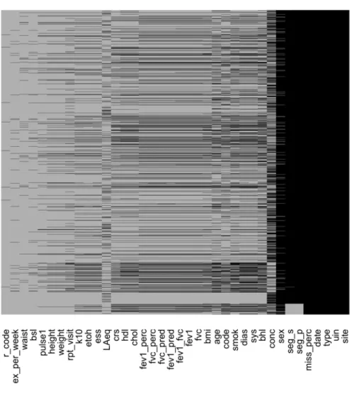
As noted earlier, the case study contained a very large amount of missing data. The overall proportion missing was 0.63. The missingness map (from the R package ‘Amelia’ [19] shown in Figure 1 displays whether data is missing (grey) or present (black), for each case.
Figure 1. Missingness map showing the amount of missing data in the case study. The horizontal axis indicates the variables in the dataset, and each
individual in the study is a row in the y-axis. Black indicates present data, grey indicates absent data.
RESULTS
As an exploratory assessment to determine whether there was sufficient missingness to warrant an investigation, t-tests and chi-squared tests were used to assess whether the presence or absence of BMI, FEV1, FVC, FEV1/FVC, and concentration, influenced either the mean values of other variables (via a t-test) or the expected count of a particular factor (via a chi-squared test). Results indicated that consistent sets of variables were affected, suggesting a potential pattern or structure of missingness. Those variables affected are listed in Table 1. These variables, and their mean values or expected counts, were reported to the industry collaborator to help explore the causes of missing data and consider down-weighting them in other analyses.
Presence/Absence of Variables affected:
BMI Date, Age, SYS, DIAS, HDL, CRS, BHL, Missing%, FEV1/FVC, FEV1%, Site, Type, SEG (P), Code, SEG (S), Rpt Visit, Smoking, Sex
FEV1, FVC, FEV1/FVC
Date, Age, SYS, DIAS, HDL, CRS, BHL, Missing%, FEV1/FVC, FEV1%, Site, Type, SEG (P), Code, SEG (S), Rpt Visit, Smoking, Sex, Ex/week
Concentration UIN, Date, Missing%, Site, Type, SEG (P), SEG (S)
Table 1. Variables affected by presence/absence of BMI, FEV1, FVC, FEV1/FVC and concentration. Date = date of examination; Age = Age at time of examination; Sys = Systolic Blood Pressure; Dias = Diastolic Blood Pressure; HDL = High Density Lipoprotein (HDL) Cholesterol; CRS = Cardiac Risk Score; BHL = Binaural Hearing Loss (%) ; Missing % = the percent of missing data in that row; FEV1% = Forced Expiratory Volume in 1 second; FEV1 / FVC = ratio of FEV1% to FVC% (FVC = Forced Vital Capacity); Site = Site the data belongs to; Type = type of data (1 = medical, 2 = follow up medical, 3 = inhalable data; 4 = respirable data; 5 = silica exposure data; 6 = noise exposure data); SEG(P) = primary SEG; Code = Medical Code; SEG(S) is the secondary SEG; Rpt Visit = Number of medical Attendances; Smoking = Smoking status of employees – current, ex, or non-smoker; Sex = Gender; Ex/week = # planned exercise sessions per week; UIN = Unique Identifying Number for an employee.
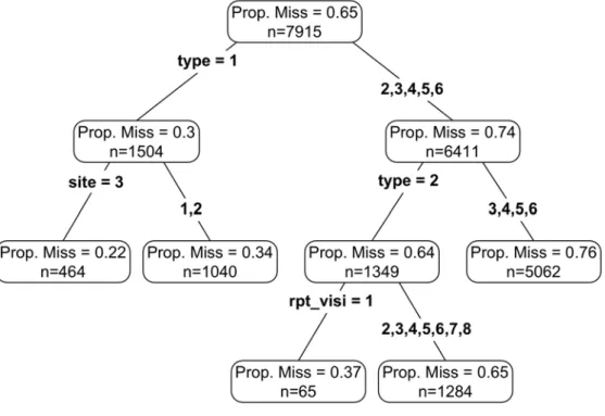
The CART and BRT models were run as described in the Method section. The CART model obtained from the analysis of the case study data is represented in Figure 2. The tree indicates that the Type of data best predicts the proportion of missing data in an individual's record. There are three main classes of data Type: medical (Type 1), follow up medical (Type 2), and hygiene or environmental exposure (Types 3-6). The missingness
proportion for each Type can be seen in the violin plot in supplementary Figure 1. The prediction from the CART model is such that when Type is 1 (medical data) there is a lower proportion of missing data (30%),
compared with the right split, when data are of Type = 2-6, (repeated medical and environmental exposure; 74% missing data). Another split occurs within Type 1, where data from site 3 has less missing data (22%) compared to sites 1 and 2 (34%). Another split occurs based on Type 2 (repeated medical data) compared to Types 3-6 (environmental exposure), where data of Type 2 has 64% missing data, and data of Type 3-6 has 76% missing data. Within Type 2 there is a split for repeated visit, such that for those with 1 visit, there is 37% missing data, and for all other visits (2-8) there is 65% missing data.
Figure 2. CART analysis of the case study data, indicating that Type of data and repeated visit (rpt-visit) are important predictors of the proportion of data missing. The three numbers in each oval indicate the expected proportion of missing data (Prop. Miss) per row of data (i.e. individual's record) and the number of rows (n). Definitions of variables used for splits are given in the captione of Table 1.
The analysis ably demonstrated the utility of this modelling
approach in identifying those variables and their values that are important for predicting missingness structure. From this model, we were able to confer with data collectors to determine that the 'Types' of data were originally separate datasets, which were then combined and represented as records for each individual (employee), resulting in many missing values per record. We were also able to identify that different variables were measured at sites 1 and 2 compared to site 3, and that repeated measures had less data as tests became more specific for subsequent visits.
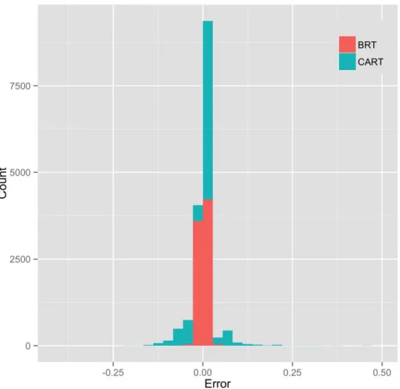
Figure 3 provides a graphical evaluation of model fit of the CART and BRT models. Figure 3a shows the predicted proportions of missing data per row based on the CART model, compared with the observed proportions. It is apparent that the model can accurately predict small and large proportions of missing data, but is less accurate at predicting
moderate proportions. This predictive resolution is a result of the trade-off between robustness, parsimony, and accuracy, reflected by the degree of pruning of the tree. Allowing more branches in the model on the right panel in Figure 3 provided a better fit to the observed data but may lead to overfitting. The predictive resolution was also a result of using a single tree rather than multiple trees [30], motivating the complementary use of
missing data from the BRT model in Figure 3b confirmed that this model provides improved goodness of fit. Figure 3c also shows that the CART and BRT models provided mostly very accurate model fits, with the BRT model having a comparatively tighter error distribution compared to the wider distribution of the CART model.
Figure 3. Comparison of observed (horizontal axis) and predicted (vertical axis) proportion of data missing per row, based on (a) the CART model (top left), and (b) the BRT model (top right). All points in these plots have a small jitter added to their position so that repeated points can be seen. The bottom panel (c) also shows the error distribution of the BRT and CART results, with both having good prediction (close to 0), and the CART model having a wider distribution.
Results from the BRT model also give the relative importance of variables in predicting the proportion of missing data; Figure 4. This analysis shows that obesity (measured by BMI) and lung function (measured by FEV1 and FVC) are the most important variables for prediction of missingness.
Figure 4. Relative Importance (RI) of variables in predicting the proportion of missing data per row based on a BRT analysis. Only variables with RI > 1 are the variables included, in order of importance (left to right) are BMI (25.57), FEV1(25.25), FEV1(Predicted) (14.22), FVC(11.34), FVC(Predicted)(6.266), Type(4.23), FEV1(Percent)(1.80), Smoking(1.66), Systolic Blood Pressure(1.58), Blood Sugar Level(1.02), K10 Depression score(1.00).
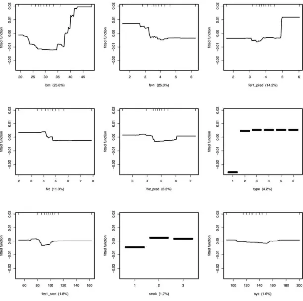
Figure 5 shows the observed proportions of missingness compared with the fitted function based on the BRT model, for the first nine variables indicated in Figure 4. The centre of the vertical axis indicates the model expected proportion of missingness. As might be anticipated, those
variables with more definite nonlinearity in the fitted function have more influence in the BRT analysis. For example, more missingness is
anticipated in individuals with higher BMI or lower lung function measurements.
Figure 5. Fitted function of variables based on the BRT model with the zero-point of the vertical axis indicating the model expected proportion of
missingness. Lines above 0.00 indicate more missingness than expected, and lines below indicate less missingness. Note that Type and smoking (smok) are
SIMULATION STUDY
Two experiments were created to explore the capability of decision tree models in elucidating the induced missingness structure.
Experiment One
In this first experiment, datasets were created where the variable instigating the missingness was either (i) not missing, or (ii) 50% MCAR. These new datasets contained five variables, two categorical and three continuous, with 1000 observations in each. The two categorical factors, F1 and F2, ranged uniformly across categories nominally labelled 7, and 1-10, respectively. The three continuous variables, C1, C2 and C3, were normally distributed with means and standard deviations of 50 and 10, 90 and 10, and 30 and 3, respectively.
These variables and values were chosen to represent specific variables in our dataset: C1: age, C2: lung function, C3: BMI, F1: SEGs, and F2: a score obtained from a measurement. The variable C1 determined whether C2, C3, F1, and F2 were missing such that when C1 was greater than 55 these variables went missing with probability 0.95. C1 was selected as the missingness instigator to mimic a scenario where someone aged 55 is not measured on a variety of variables.
The CART and BRT models were assessed on one hundred
simulated datasets for each of these two scenarios, where the outcome is the proportion of missing data in the variables C1, C2, C3, F1 and F2.
Model performance in the first experiment was evaluated based upon the criteria:
A) Did the model predict the variable, C1, as responsible for the missingness?
B) Did the model identify the threshold value of 55 for the variable C1 as the value causing the missingness?
If the models performed well in this first experiment we have confidence that the models identify structured missingness.
Experiment Two
The second experiment explored the performance of decision trees for use with MCAR data. For the second experiment the CART and BRT models were assessed on two datasets, MCAR 20%, or MCAR 50%, with one hundred simulated datasets created. In this experiment, the simulated datasets were the same as the first experiment with the addition of two variables, R1, and R2, drawn from a random uniform distribution. These last two variables were deliberately included as "noise" in the simulations
to assist in assessing whether the models are overfitting the data. In addition to the criteria used for experiment one, we assessed experiment two based upon the variance in the measures of variable importance, as we are interested in exploring whether there variables are consistently selected as important in an MCAR scenario. If this is the case, then we can assume the decision tree models are simply picking up on noise, rather than signal. These variables represent a small, simple, and realistic dataset that we would encounter at our industry site (except for variables R1 and R2 from experiment 2). The intention was to evaluate the missingness represented by our real dataset, MAR and MNAR, and compare it to data MCAR to evaluate model performance.
Variable importance was measured for each of the simulated datasets and was compared to the case study dataset. For both experiments in the simulation study, the BRT model had a smaller interaction depth of 2, rather than 5 that was used in the case study analysis, as the simulation study dataset had far fewer variables.
Simulation Study Results
In the first experiment, for both parts 1i (not missing) and 1ii (50% MCAR), the CART model identified that the variable C1 was responsible for instigating the missingness, satisfying criterion A. The CART model
also correctly identified the split for C1, such that when the threshold C1 > 55 there was an increased amount of missingness and this satisfied criterion B. All developed CART models selected C1 for the split and the value 55, meaning that all models were essentially identical. These models can be viewed in supplementary Figure 2.
Intriguingly, the BRT model was unable to identify C1 as the most important variable in predicting the proportion of missing data,
irrespective of whether C1 was not missing or 50% MCAR. Hence the BRT model did not satisfy criterion A. However, when inspecting model
predictions against variable values, the BRT model predicted a change in missingness as C1 reached 55. These fitted functions can be seen in supplementary Figure 3. This BRT model satisfied criterion B.
For the BRT model, there was variation around variable importance in this simulation study, such that when there was more missingness, there was greater variation in variable importance. An illustration of this is given in supplementary figure 4. The CART model always used C1, and the value 55 to split on, and so evaluating variable importance is somewhat
irrelevant.
For the second experiment, the data were either i) 20% MCAR, or ii) 50% MCAR. The CART model showed different levels of variable
importance over simulated datasets, and that the spurious random variables R1 and R2 were often identified as important. This can be seen in
supplementary figure 4.
The variation in variable importance was smaller in the resampled case study dataset, compared to experiment two. The BRT model, like the CART model, also chose variables R1 and R2 as relatively important in predicting missingness. Visual depictions of the variation in variable importance for the CART and BRT models over the experiment and case study data can be found in supplementary figures 6, 7, and 8.
The difference in variation of variable importance for simulated versus the resampled case study data provided evidence that data MCAR produces greater variation in variable importance. There was less variation in variable importance for simulated data compared to case study data, suggesting the case study data does have a missingness structure.
DISCUSSION
In this paper we proposed the use of decision tree models, notably CART and BRTs, for inspecting the structure of missingness in
observational data. To the authors’ knowledge this is the first time that these decision tree models have been proposed for this purpose. The
application of the models to a substantive case study involving occupational health data, specifically medical tests for employees, demonstrated the complementarity of the analyses. Whereas the CART model identified three variables: Type of medical; how many visits the employee had and site, the BRT model identified BMI and lung function as the most important factors predicting the proportion of missingness in the
employees’ health records. In addition, the BRT analysis also modelled the expected missingness for variable values.
The case study partners found that these results revealed important known and unknown structure in the data. An example of structure that was known to exist but not known to have such dominant influence, was that the dataset was a collection of smaller databases coming from different sources, denoted by the values of Type. That is, Types 1 and 2 are different kinds of medical data, and 3-6, environmental exposure data. The datasets were originally combined in this fashion so that data could be matched by ID number, allowing deidentified inspection of individual results. Where matching was not possible, group results could be observed. As a result of this concatenation of different data Types, large chunks of data were missing, as the sources collected different kinds of information and used different IDs, preventing data matching. Further exploration of the
missing data was missing for Types 3-6, compared to Types 1 and 2. This is demonstrated in the violin plot in supplementary Figure 1.
Another missing data structure revealed in our analyses was found by comparing results from the CART and BRT analyses. The focus of the CART analysis was on Type, site, and repeated visits. Compared to the CART model, the BRT analysis focused more deeply on the medical data, and highlighted that extreme values for variables such as BMI or Lung Function, had more missing data. Discussion with industry partners on these findings revealed that individuals with extreme values for
measurements such as BMI or Lung Function require follow up tests. As follow up tests are taken on a small specific set of variables relating to the particular health query or concern, they result in more missing data in the overall dataset. Discovering these missing data structures has resulted in future research being conducted on subsets of data with selection based upon these missing data structures. This allows for more representative, reliable, and valid results. It may also motivate different and more informed methods of data analysis and modelling.
In our analysis we used the proportion of missing data in a row as our response. This has the advantage of accommodating correlation between variables and providing a single, easily understood, summary
statistic for missingness. Alternative measures of missingness of the dataset could be used, such as missingness in individual variables or an index based on a factor analysis, or similar dimension reduction method. These could then be used to predict other structural features of the data, such as multiple individual variable's missingness in a multivariate analysis, or clusters of missingness, and would tell us different things about the missingness structures in the dataset.
The analysis of missing data described in this paper is not limited to decision trees and could be extended to other analyses such as neural networks, random forests, and Bayesian Learning Networks. Moreover, decision trees themselves can be implemented using different varaible selection methods, although recursive partitioning is the standard choice [24,27], As illustrated in this paper, decision trees using recursive
partitioning were desirable for ease of implementation, handling non-parametric data, and automatic handling of missing data.
It was mentioned in the introduction that knowing the structure of the missing data may not give a clear indication of the mechanism (in terms of MCAR, MAR, MNAR). However, understanding the missingness
structure can help lead the researcher to create better imputation models or use alternative methods of addressing missing data, as well as improve
future data collection or conduct their own further investigations into missingness structure, [3].
Our simulation analysis performed the decision tree analysis on MCAR and MAR scenarios to evaluate model performance using a simple, known example of missingness. In the case study, however, although MAR and MCAR variables are present, the dominant form of missingness is MNAR, due to the nature of the medical examinations. Thus the methods suggested in this paper have been demonstrated to be effective for all three types of missingness. However, as indicated in the introduction, MNAR scenarios could be envisaged whereby the data exploring the missinginess are not observed structurally. This motivates further research on this issue.
CONCLUSION
R1 C5
The use CART and BRT models have allowed us to develop our understanding of missingness structure in the data. The authors’
experience in using these models was that they motivated the appropriate questions to explore the missing data structure, leading to a better
improve both data collection and the handling of missing data in future analyses.
The results of the simulation study were surprising. Despite the a priori expectation, based on published literature, that the BRT model would be more robust and accurate than the CART model, this was not borne out in the analysis. The BRT model accurately predicted whether or not there was substantial missing data, and the diagnostic charts provided a visual indication of how missingness behaves for variables. However, in the simulation study, BRT was unable to select the correct variable as the most important for predicting the (known, modelled) missingness structure in the data. In contrast, the CART model did this consistently.
Experiment two involved the evaluation of decision tree performance on data MCAR (20% or 50%) using the simulated datasets from the first experiment with the addition of two variables, R1, and R2, drawn from a random uniform distribution. R1 and R2 were included in these simulations to assist in exploring which variables were important for splitting in the CART and BRT models when there was no structure in the missingness. Results from experiment two demonstrated that both the CART and BRT models had greater variation in variable importance when more
missingness was introduced, although this seemed to relate to the degree that the dependent variable was missing.
Although this study has demonstrated the utility in using decision tree statistical methods to identify variables and values related to missing data in a dataset, it is noted that these methods do not address whether the data is MCAR, MAR, and MNAR, and they do not specifically outline the bias that is in the data due to missingness. Instead, these methods are helpful in determining why and how data are missing. It is still up to the researcher to understand the potential bias that this may or may not cause.
Acknowledgements
The authors thank Dr. Nicole White and Dr Jegar Pitchforth for assistance and helpful discussions. The authors also thank the reviewers for their constructive comments.
Author contributions
• Mr. Nicholas Tierney had the intial idea to explore missing data using decision trees, performed all analyses, and wrote the first draft.
• Professor Kerrie Mengersen provided guidance in selecting and interpreting analyses, designing the simulation study, and critical review of manuscript.
• Dr. Fiona Harden assisted in the acquisition of data, interpretation of results from an industry perspective, and critical review of manuscript. • Dr. Maurice Harden assisted in acquisition of data, interpretation of
results from an industry perspective, and critical review of manuscript. • All authors approved the version of the paper for publishing, and
agreed to respond to questions that may arise regarding integrity of the work.
Competing Interests
The authors declare no competing interests.
Funding
This research was funded by an Australian Postgraduate Award (APA), the Australian Technology Network Industrial Doctoral Training Centre (IDTC) and the Australian Research Council.
Data Sharing Statement
Technical appendix, statistical code, and dataset available from the
corresponding author at Dryad repository, who will provide a permanent, citable and open access home for the dataset. The case study data will not be provided due to confidentiality agreements with industry partners.
SUPPLEMENTARY FIGURES
Variable Detail
site Site of work
uin unique identifying number sex gender
type type of data
date date of examination
FVC Forced Vital Capacity
FVC% FVC Percent Predicted
FEV1 Forced Expiratory Volume in 1 second
FEV1% FEV1 percent predicted
seg_p Primary Similar Exposure Group
seg_s Secondary Exposure Group
Age Age at time of medical examination BMI Body Mass Index
Code Medical Code
sys Systolic blood pressure
dias Diastolic blood pressure
hdl High Density Lipoprotein Cholesterol
chol Total Cholesterol
CRS Cardiac Risk Score
smok Smoking Status
ess Epworth Sleeping Scale k10 K10 Depression Score
etoh Alcohol Audit Score
BHL Binaural Hearing Loss
rep_vis Number of medical Attendances
ex_per_week Number of exercise sessions a week
height Height
waist Waist Circumference
bsl Blood Sugar Level
pulse Pulse Rate (bpm)
conc concentration of dust
laeq Noise
Supplementary Table 1. A list of the variables used in the decision tree analysis, and their details.
Supplementary Figure 1. Proportion of missing data per row based on the different data Types.
Supplementary Figure 2. Illustrative CART model based on the simulated data in the simulation study. The three numbers in each oval indicate the expected
proportion of missing data (Prop. Miss) per row of data, the number of rows (n) and the percentage of total data (n%) in that node. All CART plots and summaries for conditions 1A and 1B can be extracted from the code provided in supplementary material.
Supplementary Figure 3. Fitted function corresponding to the five variables considered in the simulation study, with the zero-point of the vertical axis
indicating the model expected proportion of missingness, lines above 0.00 indicate more missingness than predicted, lines below indicate less missingness. In the top row (Part A) there is no missing data in variable C1, and in the bottom row (Part B) C1 is 50% MCAR.
Supplementary Figure 4., Depicting the BRT model variable importance over all simulated datasets, where the red dots indicate when C1 is present, and the teal indicates when C1 is 50% MCAR.
Supplementary Figure 5. Variable importance for the CART model in experiment 2, where the data is MCAR 20% (red) and MCAR 50% (blue).
Supplementary Figure 6. Variable importance for the CART model when data is 80% resampled (with replacement), points have 50% transparency to help display duplicate values.
Supplementary Figure 7. Variable Importance for the BRT model, for MCAR 20% and MCAR 50%, where the red points indicate MCAR 20%, and blue indicates MCAR 50% in experiment two.
Supplementary Figure 8. Variable Importance for the BRT model, when the data is resampled 80% (with replacement).
REFERENCES
1 Greenland S, Finkle WD. A critical look at methods for handling missing covariates in epidemiologic regression analyses. American journal of
epidemiology 1995;142:1255–64.
2 Sterne JA, White IR, Carlin JBet al. Multiple imputation for missing data in epidemiological and clinical research: Potential and pitfalls. Bmj
2009;338.
3 White IR, Carlin JB. Bias and efficiency of multiple imputation compared with complete-case analysis for missing covariate values. Statistics in
medicine 2010;29:2920–31.
4 Schafer JL, Graham JW. Missing data: Our view of the state of the art.
Psychological Methods 2002;7:147–77.
doi:10.1037//1082-989X.7.2.147
5 Simon GA, Simonoff JS. Diagnostic plots for missing data in least squares regression. Journal of the American Statistical Association 1986;81:501– 9.
6 Little RJ. A test of missing completely at random for multivariate data with missing values. Journal of the American Statistical Association
7 Rubin DB. Inference and missing data. Biometrika 1976;63:581–92. 8 Virtanen TE, Lerkkanen M-K, Poikkeus A-Met al. Student behavioral
engagement as a mediator between teacher, family, and peer support and school truancy. Learning and Individual Differences 2014;36:201– 6.
9 Mitchell KE, Johnson-Warrington V, Apps LDet al. A self-management programme for cOPD: A randomised controlled trial. European
Respiratory Journal Published Online First: 2014.
doi:10.1183/09031936.00047814
10 Jamshidian M, Jalal S, Jansen C. MissMech: An r package for testing homoscedasticity, multivariate normality, and missing completely at random (mCAR). Journal of Statistical Software 2014.
11 Janssen KJ, Donders ART, Jr. FEHet al. Missing covariate data in medical research: To impute is better than to ignore. Journal of
Clinical Epidemiology 2010;63:721–7.
doi:http://dx.doi.org/10.1016/j.jclinepi.2009.12.008
12 Karahalios A, Baglietto L, Carlin JBet al. A review of the reporting and handling of missing data in cohort studies with repeated assessment of exposure measures. BMC medical research methodology 2012;12:96.
13 Karahalios A, Baglietto L, Lee KJet al. The impact of missing data on analyses of a time-dependent exposure in a longitudinal cohort: A simulation study. Emerging themes in epidemiology 2013;10.
14 Graham JW. Missing data analysis: making it work in the real world.
Annual review of psychology 2009;60:549–76.
doi:10.1146/annurev.psych.58.110405.085530
15 Little RJ. Pattern-mixture models for multivariate incomplete data.
Journal of the American Statistical Association 1993;88:125–34.
16 Hedeker D, Gibbons RD. Application of random-effects pattern-mixture models for missing data in longitudinal studies. Psychological methods
1997;2:64.
17 Unwin A, Hawkins G, Hofmann Het al. Interactive graphics for data sets with missing values - mANET. Journal of Computational and
Graphical Statistics 1996;5:113–22.
18 Templ M, Alfons A, Kowarik Aet al. VIM: Visualization and imputation of missing values. R package version 2011;2.
19 Honaker J, King G, Blackwell M. Amelia iI: A program for missing data.
Journal of Statistical Software 2011;45:1–
20 Su Y-S, Yajima M, Gelman AEet al. Multiple imputation with
diagnostics (mi) in r: Opening windows into the black box. Journal of
Statistical Software 2011;45:1–31.
21 Cheng X, Cook D, Hofmann H. MissingDataGUI. 2014. http://cran.r-project.org/web/packages/MissingDataGUI/MissingDataGUI.pdf 22 Swayne DF, Buja A. Missing data in interactive high-dimensional data
visualization. Computational Statistics 1998;13:15–26.
23 James G, Witten D, Hastie Tet al. An introduction to statistical learning. Springer 2013. http://link.springer.com/content/pdf/10.1007/978-1-4614-7138-7.pdf
24 Breiman L, Friedman J, Stone CJet al.Classification and regression trees. CRC press 1984.
25 Hastie T, Tibshirani R, Friedman J. The elements of statistical learning. Springer 2009. http://link.springer.com/content/pdf/10.1007/978-0-387-84858-7.pdf
26 Elith J, Leathwick JR, Hastie T. A working guide to boosted regression trees. Journal of Animal Ecology 2008;77:802–13. doi:10.1111/j.1365-2656.2008.01390.x
27 Therneau TM, Atkinson EJ. An introduction to recursive partitioning using the RPART routines. 1997.
28 Sutton CD. Classification and regression trees, bagging, and boosting.
Handbook of Statistics 2005;24:303–29.
29 Friedman JH, Meulman JJ. Multiple additive regression trees with application in epidemiology. Statistics in medicine 2003;22:1365–81. doi:10.1002/sim.1501
30 Breiman L. Statistical modeling: The two cultures (with comments and a rejoinder by the author). Statistical Science 2001;16:199–231.
31 R Core Team. R: A Language and Environment for Statistical Computing. Vienna, Austria: R Foundation for Statistical Computing 2014. http://www.R-project.org/
32 RStudio. RStudio. Boston, MA, USA: RStudio 2014. http://www.rstudio.org/
33 Ridgeway G. Gbm: Generalized boosted regression models. 2013. http://CRAN.R-project.org/package=gbm