Adaptive Head-to-Tail: Active Queue Management based on implicit congestion signals

Adaptive Head-to-Tail: Active Queue Management

based on implicit congestion signals

Stylianos Dimitriou, Vassilis Tsaoussidis

Department of Electrical and Computer Engineering Democritus University of Thrace

Xanthi, Greece {sdimitr, vtsaousi}@ee.duth.gr

Abstract— Active Queue Management is a convenient way to administer the network load without increasing the complexity of end-user protocols. Current AQM techniques work in two ways; the router either drops some of its packets with a given probability or creates different queues with corresponding priorities. Head-to-Tail introduces a novel AQM approach: the packet rearrange scheme. Instead of dropping, HtT rearranges packets, moving them from the head of the queue to its tail. The additional queuing delay triggers a sending rate decrease and congestion events can be avoided. The HtT scheme avoids explicit packet drops and extensive retransmission delays. In this work, we detail the HtT algorithm and demonstrate when and how it outperforms current AQM implementations. We also approach analytically its impact on packet delay and conduct extensive simulations. Our experiments show that HtT achieves better results than Droptail and RED methods in terms of retransmitted packets and Goodput.

Keywords-QoS, AQM. Packet rearrangement 1. INTRODUCTION

TCP congestion control works on the basis of exhausting the available bandwidth. In order to detect the level of available bandwidth, TCP increases gradually its sending rate, until a packet loss occurs. This way, TCP detects the maximum bandwidth allowed and retreats. As a result, congestion events occur. However, as flows enter and leave the network, the bandwidth that corresponds to each flow changes and TCP is forced to repeatedly detect the available bandwidth (i.e. its fair share). TCP versions that rely on the AIMD algorithm, such as Tahoe, Reno, and Newreno [7], detect congestion by packet losses. Unlike traditional TCP, more sophisticated variations use additional metrics beside packet loss to detect congestion. Measurement-based TCP, such as Vegas [1], Westwood [21] and Real [22] base their congestion control on passive or active measurements.

Some of the most common and easily deployable metrics are RTT, on the sender’s side, and interarrival gap, on the receiver’s side if we refer to packets and on the sender’s side if we refer to ACKs [13]. It is, thus, apparent that transport layer protocols are able to respond both to explicit (multiple DACKs and expirations of the RTO interval) and implicit (fluctuations of RTT, variable jitter etc.) congestion signals.

However, network layer mechanisms do not have the same level of sophistication. Whilst the majority of existing AQM techniques are capable to generate explicit congestion signals via packet dropping, they are unable to generate implicit congestion signals. Apart from the pure dropping-based AQM, many schemes use packet drops to set priorities among packets or flows; for example they drop lower priority packets with higher probability. Occasionally, their main objective is not to avoid a congestion event but, rather, to favor higher priority packets. Thus current AQM techniques lack mechanisms to generate implicit congestion signals, hindering transport protocols to reach their full potential.

In order to bridge the gap among highly responsive transport protocols and traditional network layer mechanisms, we introduce Head-to-Tail, an AQM technique that introduces implicit congestion signals via packet rearrangement. HtT has four main characteristics: packet rearrangement, adaptive behavior, in-order delivery and no proactive dropping. Based on a probability, Head-to-Tail moves all the packets of a specific flow from the head of the queue to its tail and as a result it increases their queuing delay and “generates” an implicit congestion signal. As more flows content for resources and more packets occupy the queue, packet rearrangement has greater impact, and the additional queuing delay inflicted becomes more perceptible. The rearrange probability is adaptive and aims at minimizing packet losses due to overflow. In order to eliminate the probability of out-of-order delivery and generation of DACKS, HtT rearranges all the packets of one flow. HtT also avoids proactive packet dropping due to its unpleasant

effects. Apart from degradation of real-time applications quality, blind packet dropping might result in loss of certain types of packets (SYN, ACK, ICMP packets) and extend significantly the connection time of short-lived flows. Instead, HtT informs indirectly the end-user on the levels of contention in the buffers.

During our work we faced four major challenges: 1. Overcome TCP heterogeneity. The heterogeneity of TCP versions reflects a corresponding heterogeneity on their levels of sophistication. Traditional TCP measures RTT only to adjust the RTO interval and detect packet losses, while more advanced approaches, based on measurements, are able to detect the level of contention with better precision. Moreover, each TCP version relies on different metrics to form its strategy: it may measure RTT values, one-way delays or interpacket gaps. Some versions are conservative (Tahoe has no fast recovery phase) while other are more aggressive (Vegas retransmits a packet after only one DACK). HtT should be able to broadly accommodate such conflicting protocol requirements, with emphasis on measurement-based protocols.

2. Reach a level of granularity that incorporates the scale of delay increments. We should be able to regulate the delay increase inflicted by HtT in order to have the desirable behavior; causing congestion window decrease without causing timeout. Namely, the additional delay should be big enough to be captured from TCP as an irregularity on measured RTT values and small enough to be below the RTO interval. This objective becomes more intricate as the sample RTT, frequently, tends to fluctuate, rendering the delay increase obsolete.

3. Balance the delay decrease caused by HtT. Since HtT rearranges the order of the packets in the queue, some packets will be favored in the final ranking and the corresponding flows will perceive a diminished queuing delay. If the perceived RTT is much smaller than expected, the flows will probe for more bandwidth and increase their rates. HtT has to incorporate a technique to regulate this delay decrease to desirable levels.

4. Surmount the “no-proactive-dropping strategy” limitations. No packet dropping may have negative effects, concerning the limited buffer capacity. Current AQM techniques use packet dropping not only to warn end-users for an upcoming congestion event, but also to alleviate the buffer load. Although HtT lacks such a packet dropping mechanism, it adapts its strategy on the amount of dropped packets due to overflow in a period of time, and specifically on the dropped to enqueued packets ratio. While this ratio is high, HtT is offensive, rearranging many packets. As this ratio decreases, HtT decreases its rearrangements.

The AIMD mechanism, that regulates the congestion window of traditional TCP, results in varying congestion window, which has, in turn, the

undesirable effect of fluctuating queue length at the router. In these cases, as we will prove later, HtT may have harmful results to end-users, resulting in multiple timeouts and retransmissions. However, since the research interest moves to sophisticated transport protocols that result in constant sending rates and stable queue lengths, more protocols will take advantage of HtT capabilities eventually. Further analysis indicates that the implementation of a transport protocol that cooperates closely with HtT is possible. Such a protocol, will be able to capture a very good approximation of the link state and respond accordingly.

The rest of the paper is organized as follows: Section 2 presents the work that has been done on the AQM schemes field. In Section 3 we outline the requirements that HtT needs to satisfy and in Section 4 we describe in detail the HtT algorithm and its various mechanisms. In Section 5 we quantify the rearrangement delay invoked by TCP, by analyzing its various components and in Section 6 we analyze the effect of TCP on queue length and relate it with TCP’s capability to detect delay variations. Section 7 includes the simulation topologies and results and in Section 8 we conclude and set the framework for future work.

2.RELATED WORK

Since 1993 when RED [8] was first proposed, researchers have investigated a plethora of mechanisms that are either dropping-based or priority-based.

Random Early Detection introduced proactive dropping so as to inform the flows that a congestion event was imminent and at the same time lower the size of the queue. The initial RED utilized two thresholds, a maximum and a minimum, which corresponded to average queue length. Every packet that arrived at the queue whose length was greater than the maximum threshold would be discarded. Considering that many packets that could otherwise be accommodated by the queue would be unnecessarily dropped, the gentle RED [17] modification extended maximum threshold to twice its value. However, although we may exploit fully the buffer space this way, packet drops do not have always desirable effects. Some applications that generate a small amount of critical data, such as Telnet, do not exit from slow start and may delay by packet drops. In [15] the authors propose for the first time ECN (Explicit Congestion Notification). In ECN packets are not dropped; instead they are marked by the router, and their marking will have the same effect on senders as packet loss. One issue with RED gateways is the lack of adaptability on different traffic levels. Adaptive RED [4], [6] avoids link underutilization by maintaining the average queue length among the two thresholds by adjusting pmax.

Another approach, Exponential-RED (E-RED) [10] sets the packet marking probability to be an exponential function of the length of a virtual queue whose capacity is slightly smaller than the link

capacity. As we see, RED and many of its variants use queue size in order to determine the level of contention. Contrary to this approach, BLUE [5] manages dropping, based on packet loss and link idle events; if the queue drops packets due to buffer overflows, BLUE increases the dropping probability, whereas if the queue becomes empty or idle, BLUE decreases the dropping probability. Loss Ratio based RED (LRED) [20] follows a similar way by measuring the latest packet loss ratio, and using it as a complement to queue length so as to dynamically adjust packet drop probability and decrease response time.

Besides AQM techniques that drop packets blindly, more sophisticated algorithms aim to penalize high-bandwidth or unresponsive flows while other offer service differentiation by treating packets according to their type. Weighted RED (WRED) [2] is designed to serve Differentiated Services based on IP precedence. Packets with a higher IP precedence are less likely to be dropped, thus high priority traffic will be delivered with higher probability than low priority. Flow RED (FRED) [9] uses per-active-flow accounting to impose on each flow a loss rate that depends on the flow’s buffer use. Unfortunately, extended memory and processor power is required for a big number of flows. On the other hand RED-PD (Preferential Dropping) [11] maintains a state only for the high-bandwidth flows.

Stochastic Fair BLUE (SFB) [5] uses mechanisms similar to BLUE and aims to identify and rate limit unresponsive flows based on accounting tables. Similar to SFB, ERUF [16] uses source quench to have undeliverable packets dropped at the edge routers. The CHOKe mechanism [14] matches every incoming packet against a random packet in the queue. If they belong to the same flow, both packets are dropped. Otherwise, the incoming packet is admitted with a certain probability. Last, NCQ [12] distinguishes data into congestive and non-congestive queuing (minimal-size) packets and favors non-congestive packets over non-congestive during scheduling.

Although HtT cannot be categorized as neither dropping-based nor priority-based AQM technique, it has some similarities with the former group of algorithms. HtT implicitly indicates congestion status to the end-nodes, not by packet loss but by packet delay. HtT can thus be considered as a new category of Active Queue Management mechanisms.

3.BASIC REQUIREMENTS

Prior to presenting the HtT implementation, it is essential to list the basic requirements which need to be satisfied. In general, HtT is oriented towards performance and, on this stage of development, does not incorporate solution for real-time traffic.

1. HtT should aim towards the decrease of unnecessary packet retransmissions. Apart from link underutilization, packet retransmissions have harmful effects on battery-powered devices, like laptops and sensors. They increase the time the

network card has to be in sending mode and they expand the total connection time. Moreover, most real-time applications are less tolerant in packet losses (since the UDP, that is usually utilized by real-time applications, does not incorporate packet retransmission mechanisms) and would accept a small delay rather than not to receive the packet at all.

2. The rearrangement algorithm should not result in out-of-order delivery. Out-of-order delivery, depending on the TCP version, usually results in packet retransmission. Let’s consider the situation in Fig. 1, where we decide to rearrange only the first packet of the queue, and move it from the head to the tail (packets a and b belong to the same connection). If these two packets belong to a TCP Vegas flow, when the packet ‘b’ arrives at the receiver it will trigger the generation of a DACK for packet ‘a’. TCP Vegas will respond to this DACK with an immediate packet retransmission, even though no loss has occurred. Typically, 3 DACKs are required.

3. HtT needs to associate its strategy with the level of contention, namely adjust its rearrangement probability as flows enter and leave the network. Unlike RED and some of its variants that take into account the queue length, HtT’s mechanism is self-adjustable. The significance of rearrangement depends strictly by the number of packets presently in the queue; no extra action has to be taken.

Figure 1. Rearranging the first packet of the queue.

4.BASIC HTTSCHEME

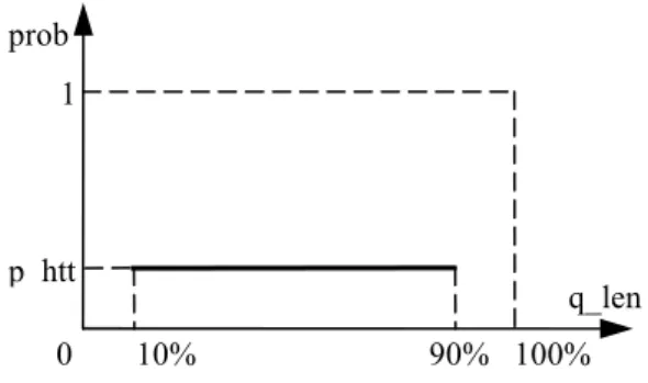
HtT’s main component is a Rearrange Probability Function (RPF), which is a function of the actual queue length (Fig. 2). As we notice, the RPF is a pulse function and defines that rearrangements may happen only when the queue is 10%-90% full. This can be explained intuitively and shows off the need to avoid too small or too big additional queuing delays. Nevertheless, the choice of a pulse function may be questionable. One might expect that an increasing function would be more appropriate, since, as the queue size is increased the function should be able to notify more flows. However, the rearrangement function does not carry a binary congestion signal as the dropping function; that is, many rearrangements

a b

a

do not have similar effect as many drops. Besides, although we will analyze extensively this remark later, we note for now that there is a hidden increase as more packets arrive at the queue. Though, instead of notifying more flows, we notify the same number of flows more explicitly. It is obvious from Fig. 1 that as the queue size increases, the additional queuing delay is also increased and the effect for the end-nodes is more significant. A first approach on the packet rearrangement scheme is in [3]. In the same paper there is an experimental justification of the choice of the pulse RPF. The p_htt variable defines the probability that some packets will be rearranged and varies depending on the router state (the initial value is 0.1).

Figure 2. The Rearrange Probability Function.

HtT’s operation is rather simple. For every packet that is ready to be served the router generates a random number between 0 and 1. If this number is smaller than p_htt then the router rearranges the head and some other packets (more details in Subsection 4.1), otherwise it routes the head and moves to the next packet.

Besides the basic scheme, HtT performs many functions that need to be discussed in detail separately, namely the rearrange function, the marking function and the adaptation function.

4.1 Rearrange function

As we mentioned in the introduction, each rearrangement consists of moving all the packets of a specific flow from their position in the queue to the tail. HtT examines the transport and network layer headers of the head and extracts the ‘addressing information’ of the packet, i.e. the (IP address, port number) pair. These fields indicate the connection/flow the packet belongs, that is the unique connection between two communicating end-nodes. Although this operation has some processing cost, the router does not keep a state; it only uses this information once. After rearranging the head, HtT scans all the packet of the queue starting from the head towards the tail and reads their flow. If they belong to the same flow as the head, then they are moved to the tail. We show the pseudo-code of the algorithm below. We use the following functions;

flow(pkt): returns the flow that pkt belongs rearrange(pkt): moves the pkt from its current position to the tail of the queue

packet(n): returns the packet that belongs on the n-ith place on the queue, where n=0 is the head no_pkts(): returns the total number of packets currently populating the queue

n=0 hf=flow(packet(n)) rearrange(packet(n)) do { n=n+1 pf=flow(packet(n)) if (hf==pf) then rearrange(packet(n)) } while(n<no_pkts())

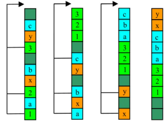
Figure 3. Rearranging packets with HtT.

Fig. 3 depicts how the rearrangement scheme works. Packets 1, 2 and 3 all belong to the same flow. HtT picks the head, reads the flow that it belongs and moves the packet to the tail. Then it scans the entire queue from the beginning to the end, searching for packets that belong to the same flow as the head. If it finds one, it moves it to the tail and repeats until it reaches to the end of the queue.

An actual implementation of the algorithm would have to face a lot of practical problems. The first is the difficulty to characterize accurately a flow and detect which packets belong to this flow. Due to Network Address Translation (NAT) [18], which is frequent in IPv4 networks, the pair of sender/receiver IP addresses is not enough to characterize a single connection. In order to identify exactly a connection we also need the pair of sender/receiver ports, as well as the transport protocol used. However, extracting more information for the packet renders the algorithm complicated and thus time-consuming. None the less, HtT is based on packet delay, so a time-consuming algorithm would contribute to the total increase of queuing delay, as long as we do not have outgoing link underutilization. If the algorithm is proved to be very heavy, we could implement it in a way that the router sends packet while scanning the queue. The implementation details of such a solution are beyond the scope of this work. An other apparent solution is to this problem is to assume that the pair of IP addresses can characterize a single connection, an assumption which will be more valid in the future as IPv6 users are increased. Even though on edge-routers

1 2 3 1 2 3 1 2 3 2 3 1 0 prob 1 100% p_htt 10% 90% q_len

such an approach is unrealistic, for example, many computers behind a company’s router that uses NAT may communicate with the same server, the worst case scenario is the router rearranging all the incoming packets, thus adding only a little processing delay for each packet.

We should note that, this way, rearranging the packets of a single connection, HtT will add different amount of queuing delay for different packets of the same flow and will eliminate any interpacket gap that might have occurred by the router’s multiplexing algorithm. Different transport protocols (or versions of well known transport protocols, such as TCP) might interpret differently the measured delays of the packets. A given transport protocol might consider that zero interpacket gap means little traffic and increase the congestion window, without taking into account that the average queuing delay has increased.

4.2 Adaptation Function

Using the same rearrange probability might work well in cases with a constant number of users, but as flows enter and leave the network, we should follow a more dynamic strategy. Our aim is not to limit the queue size to a threshold, but to minimize the packet drops caused by congestion events and specifically the portion of dropped-to-enqueued packets. We measure the number of packets arrived in the queue and the number of packets dropped due to overflow for one second. If the dropped-to-enqueued ratio measured recently is greater than the previous one, then the rearrange probability is multiplicatively increased, otherwise decreased. If the two ratios are the same, then this almost always means that there are not dropped packets in neither case, so we decrease the rearrange probability. To describe in pseudo-code the algorithm, we use the following variables and functions;

p_htt: indicates the rearrange probability of HtT enqueued: is increased whenever a packet is successfully enqueued by the queue

dropped: is increased whenever a packet is dropped by the queue due to overflow

now(): returns the current time in seconds

if(now()-last==1) { new_ratio=dropped/enqueued if(new_ratio>old_ratio) then p_htt=p_htt*1.1 else p_htt=p_htt/1.1 old_ratio=new_ratio last=now() enqueued=0 dropped=0 }

One critical difference of dropping-based AQM schemes against HtT is that as more packets are dropped, more flows are notified by the increasing contention signal. However, with HtT, after a specific

point, the impact of increased queuing delay diminishes as more and more packets are being rearranged. In Fig. 4 we have 3 flows, which have packets (1,2,3), (a,b,c) and (x,y).

Figure 4. The resulting queue with too many rearrangements.

If we do not limit the rearrange probability to a maximum value, in case of a gradually increasing contention, the probability will take big values like 0.7 or 0.8. In such a case there will be little effect on the packets and the router might not be able to return to the previous state. In order to avoid such a reaction, we will limit the maximum rearrange probability deterministically to 0.2, based on sample measurements.

4.3 Marking function

Rearranging a packet on the queue has double effect. The first is that the queuing delay of this packet is increased significantly, depending by its position in the queue. The second is that all the other packets have their queuing delay slightly decreased since now their waiting time in the router is smaller (we will cover this aspect later). In order to avoid an excessive delay for a packet that may result in expiration of the retransmission timeout, we should limit the maximum number of times a packet could be rearranged. HtT defines that a packet can be rearranged, at the very most, only once per router. In order for the router to keep track of the packets that have been rearranged, it should have a way to ‘remember’ which packets it has rearranged, i.e. implement a marking function. This marking has no relation to the marking function implemented by ECN; it refers to marking a packet while it is in the router and unmarking it when it departs. Thus the packet remains the same from hop to hop. Marking in HtT can be implemented in two ways.

1. Mark each packet separately. Using this approach, the router marks the rearranged packet in the header, usually by altering one unused bit in the Options field. When this packet becomes again the head of the queue, the router knows that this packet has been rearranged once and hence should not be rearranged again. Before the packet departs from the queue, the router alters the same bit and sends the packet to the next router. The advantages are that the router doesn’t need to keep track in a separate data structure the packets rearranged, and

2 3 a b y x c 1 1 b 1 x c 2 y 3 a y a 3 2 b 1 c x y a 3 x 1 2 b c

that it doesn’t need to alter the Header checksum of the field, since the packet returns to the previous state before moving to the next router. 2. Maintain separate data structure. This way we

have an array or a list where we record the connections whose packets have been rearranged and the number of packets for each connection; any other information, e.g. sequence number, is unnecessary. When a packet leaves the queue, the router just needs to examine the flow it belongs and either decrease by one the total number of packets, or erase the record if this is the last packet of the flow. The packets are not affected and the process of identifying the already rearranged packets is faster. Unfortunately, a memory consuming data structure should be created. Both these approaches are semi-stateless, in the sense that we don’t have to maintain a large reference table for all the flows in the network. Only the flows whose packets currently occupy the router are recorded for a small period time. During our evaluation of the technique we followed the first approach.

5.ANALYSIS OF REARRANGEMENT DELAY

In Section 4 we saw that the effect of HtT on packets is twofold; some packets gain additional delay, while the rest take higher priority in the queue.

We will continue by analyzing the effect on the additional queuing delay on a per hop perspective. At the end of the analysis we end-up with a sum (dHtT++dHtT-), which indicates the delay factor inflicted

by HtT to a packet. If this factor is positive it should be big enough to be perceived as an indication of increased contention. On the other hand, if it is negative, it should be so small that would not be perceived as an indication of small contention levels; otherwise the sender might increase its rate.

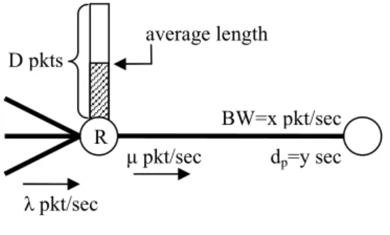
We consider a link (Fig. 5). We summarize our definitions in Table 1. We also consider λ>µ (in this case the service rate equals to the bandwidth of the link) and we assume that all packets have fixed length. We deliberately omit processing delay from our analysis. Processing delay can be an important part of the total delay since the router has to examine the network and transport layer header for every packet to decide if it will rearrange it, and then, if it decides to rearrange it, it has to examine the headers of every other packet in the queue.

TABLE 1. LINK CHARACTERISTICS Link characteristics

x packets/sec Channel bandwidth

y sec Propagation delay

D packets Router storage capacity λ packets/sec Average arrival rate µ packets/sec Average service rate

leni Average queue length

Figure 5. Channel characteristics.

On a per hop perspective, the total delay of a packet consists of four delays:

dp: propagation delay

dt: transmission delay

dq: queuing delay

dpr: processing delay

We will ignore processing delay for now. On HtT gateways, we have two more delay components:

dHtT+: the additional delay inflicted by HtT

dHtT-: denotes the decrease of the queuing delay

caused by the rearrangement of other packets. We consider an arriving packet at the queue. If leni

is the length of the queue the time the packet arrives, we have:

sec

d

=

y

1 pkt

1

=

sec

pkt/sec

d

x

x

=

sec

avg

d

len d

x

=

⋅

=

In HtT gateways, we have two possibilities; either a packet is rearranged or not. If the packet is rearranged, it will gain an additional queuing delay, dHtT+. Regardless of the packet’s rearrangement, other

packets might be rearranged in the queue as well. In case other packets are rearranged, for each packet rearrangement, the waiting time of the packet will be diminished by a delay equal to the transmission delay of one packet. The total decrease of the queuing delay in that case is the dHtT- factor. In reality, things are

more complex since each rearranged packet has different dHtT+ and the effect on the entire congestion

window is cumulative; however, at present, we emphasize on the delay impact of HtT on a single packet.

We considered earlier a packet that arrives at a router with queue length equal to leni. After a time

equal to the queuing delay dq, all the previous packets

have been routed and the packet is the first to be served. During this time, more packets have arrived at the router. Thus the current length of the queue is:

R BW=x pkt/sec dp=y sec λ pkt/sec µ pkt/sec average length D pkts

(

)

pkts

length i

q

=

len

+ ⋅

x

λ µ

−

If, at this point, the router decides to rearrange that packet, the queuing delay will increase by the expected delay of the packet. If A+ is a variable that

corresponds to the combined probability of rearrangement and the present position of the packet in the queue, this additional delay equals to:

(

)

1

sec

sec

d

A

len

x

x

len

d

A

x

λ µ

λ µ





=

⋅



+ ⋅

−



⋅

⇔





=

⋅



+ −







Most of the times, a rearranged packet is the head of the queue, however sometimes it may be rearranged from the ‘body’ of the queue. For our current analysis we consider that the rearranged packet is the head.

At the same time, the packet might be favored by a waiting time equal to several transmissions delays. If A- is a factor that includes both the probability and the

number of rearrangements of other packets, the sum of these delays is:

1

sec

d

A

x

= −

⋅

The total delay for a packet now becomes:

total p t q pr HtT HtT

d

=

d

+

d

+

d

+

d

+

d

+

d

x

A

x

len

A

x

len

x

y

d

1

1

⋅

−













+

−

⋅

+

+

+

=

λ

µ

Eq. (8) describes generally the total delay for a packet. If A+=0 then the delay increase due to HtT is

zero, that is the packet is not rearranged in this hop. If both A+ and A- are zero, then during the time period

that the packet is in the queue, the router rearranges no packet, thus causes neither delay increase nor decrease for no packet. The last two elements of Eq. (8) also indicate the required level of granularity of the transport protocol in order to capture the extra queuing delay caused by HtT. The sum (dHtT++ dHtT-)

should be significant enough to signal increased contention. In cases of smaller contention, it should approach zero.

Moreover, the aforementioned expression of packet delay, which is an equation of x, y and leni,

indicates the conditions under which HtT has its optimal performance, that is the conditions under which current TCP implementations can capture the variations of queuing delay. Topologies with small propagation delays or big buffer spaces are ideal for HtT operation. Leni corresponds to the expected

average length of the queue, in this way we would expect bigger leni for routers with greater buffer

capacity.

6. AVERAGE QUEUE LENGTH

In Eq. (8), leni indicates the length of the queue

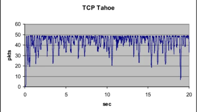
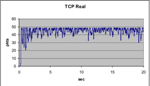
the moment a random packet arrives. None the less, the queue length is mostly determined by the number of flows and the underlying transport protocol. AIMD-based TCP variations tend to create queues whose length fluctuates whereas more sophisticated TCP variations maintain stable queue lengths. Using a dumbbell topology with 20 flows, we observed the length of the queue of the bottleneck link for 20 seconds. TCP Tahoe 0 10 20 30 40 50 60 0 5 10 15 20 sec p k ts

Figure 6. Queue length with TCP Tahoe flows.

TCP Newreno 0 10 20 30 40 50 60 0 5 10 15 20 sec p k ts

Figure 7. Queue length with TCP Newreno flows.

TCP Vegas 0 10 20 30 40 50 60 0 5 10 15 20 sec p k ts

TCP Real 0 10 20 30 40 50 60 0 5 10 15 20 sec p k ts

Figure 9. Queue length with TCP Real flows.

As we observe in Figs. 6-9, depending on the congestion control implemented, the queue may heavily fluctuate - in case of AIMD-based TCP - or may have a more stable behavior - in case of more sophisticated TCP versions.

The queue length corresponds to queuing delay. Stable queue length results to stable queuing delay. Flows that base their strategy on RTT measurements measure values with small deviation and thus they tend not to modify significantly the sending rate. In these cases the delay caused by HtT can be easily captured by TCP as an unexpected additional delay. On the other hand, fluctuating queue lengths have the disadvantage that instant small values of RTT, combined with a decrease of the queuing delay dHtT-,

might trick the protocol to think that there is link underutilization and lead to a congestion window increase and inevitably to a congestion event. This uncertainty on the expected packet delay for the AIMD-based TCP, combined to the fact that it bases its operation, almost exclusively, to packet losses, renders HtT mechanism obsolete if not damaging to this category of protocols. In most extreme cases, a randomly high packet delay with HtT delay may lead to an expiration of RTO and unnecessary retransmissions.

7.SIMULATIONS

In this section, we present performance evaluation based on simulations. HtT has been implemented in ns-2 and is compared to Droptail and RED. HtT is tested with two measurement-based TCP variations; one sender-oriented - TCP Vegas - and one receiver-oriented - TCP Real. Although none of these protocols can cooperate perfectly with HtT, their functionality allows them to take advantage of the extra delay. We will review briefly their algorithms.

Contrary to TCP Reno, Vegas has differentiated congestion avoidance and recovery mechanisms. TCP Vegas introduces baseRTT which is the smallest measured RTT during one connection and represents the packet delay without queuing delay. It then computes two throughputs, the Actual, which is the actual throughput of the sending process, and the Expected, which is an ideal throughput with no queuing delay and equals to windowSize/baseRTT (windowSize is almost always the congestion

window). The difference diff=Expected-Actual indicates the extra, in-fly data of the flow. We consider two thresholds α and β where α<β. If diff is less than α then the flow increases its sending rate. If diff is less than β then it decreases its sending rate and if it falls between these two thresholds then it keeps the same sending rate. Vegas also favors less out of order delivery because it resends a packet immediately after just one DACK, instead of three.

TCP Real is a receiver-oriented protocol, using the notion of wave, introduced in [19]. The wave is the congestion window with three more characteristics; its size is constant during an RTT, it is advertised to both the sender and the receiver and it is determined by the pace of arriving packets at the receiver, not by the pace of ACKs at the sender. The less the contention in the channel, the greater is the level of the wave. In this wave, TCP has not only a binary knowledge of the link state, but also knows the exact level of contention. Apart from the above, TCP Real has also improved recovery mechanisms and can detect the nature of packet losses (congestion, transient errors, handoffs) and respond accordingly.

During the simulations we omitted AIMD-based TCP, such as Tahoe, Reno or Newreno. The reason is that these variations only measure RTT in order to adjust their RTO interval and not to adjust their transmission strategy. However, although Vegas and Real do not comply exactly with HtT specifications, they give us a good idea of the protocol’s performance. One last remark is that while we are mostly interested on retransmitted packets, which is the main quantity we wish to decrease, we present also results on received packets (Goodput) as well as fairness. Although the differences are marginal, we emphasize that HtT in many cases can increase performance while maintain high Fairness.

7.1 Simulation metrics

In order to evaluate HtT, we use three criteria: Received packets, Retransmitted packets and Fairness. Received packets are the packets successfully received by the receivers and retransmitted packets are the packets that were dropped by the network layer mechanisms and were retransmitted again. The reason we use packets instead of Goodput or Throughput, is that we consider that the users are active during the span of the simulation, which is 50 s. In this way, packets and rate indicate the same thing. The Fairness index we used is the Jain’s index. Since our current study does not involve real-time applications, we do not include metrics as jitter or interpacket gap.

7.2 Dumbbell simulations

The first simulation topology is a dumbbell topology with 100 flows (Fig. 10). During three sets of simulations we vary the propagation delay and the bandwidth of the bottleneck link, as well as the buffer capacity of the router.

Figure 10. Dumbbell topology. 7.2.1 Varying propagation delay

In this first set of simulations we consider a 100 Mbps bottleneck link and a router with 100 packets capacity. We then vary the propagation delay from 1 ms to 30 ms. Figs. 11 and 12 depict the results on retransmitted packets, 13 and 14 on received packets and 15, 16 on Fairness. TCP Ve gas 0 10000 20000 30000 40000 50000 1 5 10 15 20 25 30 msec R e tP a c k s DT RED HtT

Figure 11. Retransmitted packets with varying propagation delay and TCP Vegas flows.

TCP Re al 0 5000 10000 15000 20000 25000 30000 1 5 10 15 20 25 30 msec R e tP a c k s DT RED HtT

Figure 12. Retransmitted packets with varying propagation delay and TCP Real flows.

TCP Ve gas 590000 595000 600000 605000 610000 615000 620000 625000 1 5 10 15 20 25 30 ms R e c P a c k s DT RED HtT

Figure 13. Received packets with varying propagation delay and TCP Vegas flows. TCP Real 580000 590000 600000 610000 620000 630000 1 5 10 15 20 25 30 ms R e c P a c k s DT RED HtT

Figure 14. Received packets with varying propagation delay and TCP Real flows. TCP Vegas 0 0.2 0.4 0.6 0.8 1 1.2 1 5 10 15 20 25 30 ms F a ir n e s s DT RED HtT

Figure 15. Fairness with varying propagation delay and TCP Vegas flows. TCP Real 0 0.2 0.4 0.6 0.8 1 1.2 1 5 10 15 20 25 30 ms F a ir n e s s DT RED HtT

Figure 16. Fairness with varying propagation delay and TCP Real flows.

The simulation results can be partly explained by the Eq. (8). As we increase the propagation delay, the delay caused by rearrangement becomes less and less significant and the decrease on retransmitted packets is very small for big values of propagation delay.

7.2.2 Varying bandwidth

In this second set, we consider a bottleneck link with 30 ms propagation delay (the worst case from the previous scenario) and 100 packets buffer capacity.

TCP Ve gas 0 5000 10000 15000 20000 25000 20 40 60 80 100 Mbps R e tP a c k s DT RED HtT

Figure 17. Retransmitted packets with varying bandwidth and TCP Vegas flows. TCP Re al 0 2000 4000 6000 8000 10000 12000 14000 20 40 60 80 100 Mbps R e tP a c k s DT RED HtT

Figure 18. Retransmitted packets with varying bandwidth and TCP Real flows. TCP Vegas 0 100000 200000 300000 400000 500000 600000 700000 20 40 60 80 100 Mbps R e c P a c k s DT RED HtT

Figure 19. Received packets with varying bandwidth and TCP Vegas flows. TCP Real 0 100000 200000 300000 400000 500000 600000 700000 20 40 60 80 100 Mbps R e c P a c k s DT RED HtT

Figure 20. Received packets with varying bandwidth and TCP Real flows. TCP Vegas 0 0.2 0.4 0.6 0.8 1 1.2 20 40 60 80 100 Mbps F a ir n e s s DT RED HtT

Figure 21. Fairness with varying bandwidth and TCP Vegas flows.

TCP Real 0 0.2 0.4 0.6 0.8 1 1.2 20 40 60 80 100 Mbps F a ir n e s s DT RED HtT

Figure 22. Fairness with varying bandwidth and TCP Real flows.

Eq. (8) indicates that as the bandwidth of the link increases, the delay caused by HtT becomes inconsiderable. If we consider λ≈x, A+=1, leni=80 and

100 Mbps bandwidth we have dHtT+=6.4 ms and if

bandwidth equals to 20 Mbps than dHtT+=32 ms. We

can see thus that even for a 100 Mbps bandwidth link, dHtT+ is important. In the first case, the one-way delay

without HtT is 36.48 ms, the RTT is almost 72.96 ms and HtT adds an 8.7% to the total delay. In the last case, HtT adds a 25.7% to the total delay.

7.2.3 Varying buffer capacity

In the third set of simulations we vary buffer size. As expected, bigger buffers have better results in decreasing the number of retransmitted packets.

TCP Ve gas 0 5000 10000 15000 20000 25000 100 150 200 250 300 packs R e tP a c k s DT RED HtT

Figure 23. Retransmitted packets with varying buffer capacity and TCP Vegas flows.

TCP Re al 0 2000 4000 6000 8000 10000 12000 14000 100 150 200 250 300 packs R e tP a c k s DT RED HtT

Figure 24. Retransmitted packets with varying buffer capacity and TCP Real flows. TCP Vegas 618000 619000 620000 621000 622000 623000 100 150 200 250 300 packs R e c P a c k s DT RED HtT

Figure 25. Received packets with varying buffer capacity and TCP Vegas flows. TCP Real 550000 560000 570000 580000 590000 600000 610000 620000 630000 100 150 200 250 300 packs R e c P a c k s DT RED HtT

Figure 26. Received packets with varying buffer capacity and TCP Real flows. TCP Vegas 0 0.2 0.4 0.6 0.8 1 1.2 100 150 200 250 300 packs F a ir n e s s DT RED HtT

Figure 27. Fairness with varying buffer capacity and TCP Vegas flows. TCP Real 0 0.2 0.4 0.6 0.8 1 1.2 100 150 200 250 300 packs F a ir n e s s DT RED HtT

Figure 28. Fairness with varying buffer capacity and TCP Real flows.

During the last years there is a debate about the optimal size of router buffers and their effect on network utilization. We do not ignore this debate; but instead we note that (i) the buffer size depends also on the network size and DxB product and therefore, buffers can occasionally grow large even when the design is conservative; (ii) we explicitly state that the bigger the buffer, the more noticeable the delay is.

7.3 Cross-traffic simulations

Now we will make some simulations with a cross traffic topology (Fig. 29). We have 3 groups of senders, S1x, S2x and S3x and 3 groups of corresponding receivers, R1x, R2x and R3x.

Figure 29. Cross-traffic topology.

We increase the number of users from 50 for each group to 100. In this case we do not depict the results of simulations with RED because its performance is poor in the specific topology.

TCP Ve gas 0 5000 10000 15000 20000 25000 30000 150 180 210 240 270 300 flows R e tP a c k s DT HtT

TCP Re al 0 5000 10000 15000 20000 25000 150 180 210 240 270 300 flows R e tP a c k s DT HtT

Figure 31. Retransmitted packets with TCP Real flows.

TCP Ve gas 928000 929000 930000 931000 932000 933000 934000 150 180 210 240 270 300 flows R e c P a c k s DT HtT

Figure 32. Received packets with TCP Vegas flows.

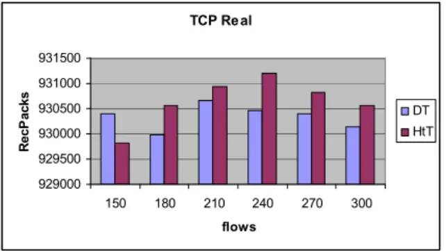
TCP Re al 929000 929500 930000 930500 931000 931500 150 180 210 240 270 300 flows R e c P a c k s DT HtT

Figure 33. Received packets with TCP Real flows.

Fairne ss 0 0.2 0.4 0.6 0.8 1 1.2 150 180 210 240 270 300 flows F a ir n e s s DT HtT

Figure 34. Fairness with TCP Vegas flows.

Fairness 0 0.2 0.4 0.6 0.8 1 1.2 150 180 210 240 270 300 flows F a ir n e s s DT HtT

Figure 35. Fairness with TCP Real flows.

As the number of users increases Goodput increases and unnecessary data transmission is avoided. This leads us to the conclusion that HtT works better under heavy contention conditions.

7.4 TCP Vegas vs TCP Real

Both TCP Vegas and Real can get significant improvements from HtT’s delay mechanisms. However, while Real has a smooth behaviour, Vegas is unpredictable as network conditions change (Figs. 23 and 24). This is due to the fact that Vegas is parameter sensitive; it depends heavily on the values of α and β, which define the thresholds between which the sending rate is allowed to fluctuate. For this reason, there are some “optimal” topologies which allow Vegas algorithm to operate with its full potential, while other topologies with slight differences may cause dysfunctions. On the other hand, TCP Real does not have such dependencies and does not rely strongly to the underlying topology. Thus, it is more scalable and can exploit better the network resources.

Moreover, Vegas and Real have different results because they measure different things. Vegas measures the RTT while Real measures the one-way delay. Thus the positive and negative effects of HtT are captured more easily by Real. TCP Real then informs the sender from the exact level of the contention, which if A+=0 and A-≠0 (Eq. (8)) will

seem to be lower than usual and will trigger the increase mechanism of the sender. Contrary to Real, Vegas not only captures less easily the additional delay but also is tolerant for relatively small decreases of the RTT.

8.CONCLUSION AND FUTURE WORK

In this paper, we reviewed and revised the HtT technique. We analyzed its operation and evaluated its performance. We demonstrated with simulations how HtT can decrease the burden of retransmitted packets in the network. In many cases, HtT can induce additional delay to packets, transport protocols can detect it and react accordingly.

Continuing our theoretic work, we study the effect of the algorithm when used on different levels on the network. Is it preferable to use HtT only on the core routers where delays are greater, or should we use it

only on edge routers where packet flow is lower? Furthermore, what are the effects on fairness when we rearrange both UDP and TCP flows? An interesting point to examine is the level of service differentiation we can achieve if we rearrange only TCP flows, and not UDP. Moreover, we work on the creation of a transport layer protocol, probably a TCP variant that will have the appropriate level of sophistication to cooperate with HtT. Having defined the granularity of the transport protocol in order to achieve maximum performance, we can get a rough idea of the protocols structure.

The next obvious step is the implementation of the algorithm in an actual network. Since processing delay is a factor that may affect seriously the performance of HtT, it is vital to move along to an actual implementation of the code to verify the correspondence of simulation data to actual results, as well as to examine any complexities that might arise. Is processing delay significant enough to eliminate the problem of delay decrease we studied earlier? If it is bigger than expected, are there ways to abate it, for example with more sophisticated scheduling? The implementation is also crucial for testing HtT with real-time applications whose performance depends mainly on the user-perceived quality and not on transmission metrics.

REFERENCES

[1] Brakmo et al, TCP Vegas: New Techniques for Congestion Detection and Avoidance, Proceedings of ACM SIGCOMM, London, UK, August 1994.

[2] Technical Specification from Cisco, Distributed Weighted Random Early Detection, URL: http://www.cisco.com/ univercd/cc/td/doc/product/software/ios111/cc111/wred.pdf. [3] S. Dimitriou, V. Tsaoussidis, Head-to-Tail: Managing

Network Load through Random Delay Increase, Proceedings of IEEE ISCC, Aveiro, Portugal, July 2007.

[4] W.C. Feng, D. Kandlur, D. Saha, K. Shin, A Self-Configuring RED Gateway, Proceedings of IEEE Infocom, New York, Usa, March 1999.

[5] W. Feng, D. Kandlur, D. Saha, K. Shin, Blue: A New Class of Active Queue Management Algorithms, U. Michigan CSE-TR-387-99, April 1999.

[6] S. Floyd, R. Gummadi, S. Shenker, Adaptive RED: An Algorithm for Increasing the Robustness of RED’s Active Queue Management, August 2001.

[7] S. Floyd, T. Henderson, A. Gurtov, The NewReno modification to TCP’s fast recovery algorithm, RFC 3782, April 2004.

[8] S. Floyd, V. Jacobson, Random Early Detection Gateways for Congestion Avoidance, IEEE/ACM Transactions on Networking, 1(4):397-413, August 1993.

[9] D. Lin, R. Morris, Dynamics of Random Early Detection, Proceedings of ACM SIGCOMM, Cannes, France, September 1997.

[10]S. Liu, T. Basar, R. Srikant, Exponential-RED: A Stabilizing AQM Scheme for Low- and High-Speed TCP Protocols, IEEE/ACM Transactions on Networking, Volume 13, Issue 5, October. 2005.

[11]R. Mahajan, S. Floyd, “Controlling High Bandwidth Flows at the Congested Router”, Proceedings of ICNP, California, USA, November 2001.

[12]L. Mamatas, V. Tsaoussidis, A new approach to Service Differentiation: Non-Congestive Queuing, Proceedings of CONWIN, Budapest, Hungary, July 2005.

[13]L. Mamatas, V. Tsaoussidis, C. Zhang, BOTTLENECK-QUEUE BEHAVIOR: How much can TCP know about it?, Proceedings of INC, Samos, Greece, July 2005.

[14]R. Pan, B. Prabhakar, K. Psounis, CHOKe: a stateless AQM scheme for approximating fair bandwidth allocation, Proceedings of IEEE Infocom, Tel Aviv, Israel, March 2000. [15]K. Ramakrishnan, and S. Floyd, A Proposal to Add Explicit

Congestion Notification (ECN) to IP, RFC 2481, January 1999.

[16]A. Rangarajan, A. Acharya, ERUF: Early Regulation of Unresponsive Best-Effort Traffic, Proceedings of ICNP, Toronto, Canada, October 1999.

[17]V. Rosolen, O. Bonaventure, G. Leduc, A RED discard strategy for ATM networks and its performance evaluation with TCP/IP traffic, ACM Computer Communication Review, July 1999.

[18]P. Srisuresh, M. Holdrege, IP Network Address Translator (NAT) Terminology and Considerations, RFC 2663, August 1999.

[19]V. Tsaoussidis, H. Badr, R. Verma, Wave and Wait Protocol: An energy-saving Transport Protocol for Mobile IP-Devices, Proceedings of ICNP, Toronto, Canada, October 1999. [20]C. Wang, B. Li, Y. Hou, K. Sohraby, Y. Lin, LRED: A

Robust Active Queue Management Scheme Based on Packet Loss Ratio, Proceedings of IEEE Infocom, Hong Kong, March 2004.

[21]A. Zanella, G. Procissi, M. Gerla, M. Y. Sanadidi, TCP Westwood: Analytic Model and Performance Evaluation, Proceedings of IEEE Globecom, Texas, USA, December 2001.

[22]C. Zhang, V. Tsaoussidis, TCP-Real: Improving Real-time Capabilities of TCP over Heterogeneous Networks, Proceedings of NOSSDAV, New York, USA, June 2001.