Toward autonomous underwater mapping in partially structured 3D environments

(1)

The author hereby grants to MIT and WHOI permission to reproduce and to distribute publicly paper and electronic copies of this thesis document in whole or

in part in any medium now known or hereafter created.

Mark VanMiddlesworth 2014. All rights reserved.

(2)

(3)

Toward autonomous underwater mapping in partially

structured 3D environments

by

Mark VanMiddlesworth

Submitted to the Department of Electrical Engineering and Computer Science on January 31, 2014, in partial fulfillment of the

requirements for the degree of Master of Science

Abstract

Motivated by inspection of complex underwater environments, we have developed a system for multi-sensor SLAM utilizing both structured and unstructured environ-mental features. We present a system for deriving planar constraints from sonar data, and jointly optimizing the vehicle and plane positions as nodes in a factor graph. We also present a system for outlier rejection and smoothing of 3D sonar data, and for generating loop closure constraints based on the alignment of smoothed submaps. Our factor graph SLAM backend combines loop closure constraints from sonar data with detections of visual fiducial markers from camera imagery, and produces an on-line estimate of the full vehicle trajectory and landmark positions. We evaluate our technique on an inspection of a decomissioned aircraft carrier, as well as synthetic data and controlled indoor experiments, demonstrating improved trajectory estimates and reduced reprojection error in the final 3D map.

Thesis Supervisor: John Leonard

(4)

(5)

Acknowledgments

They say “it takes a village...,” and sometimes I wonder what it would be like if my academic support network were an actual village. I like to think of it as a pre-Columbian settlement in, say, the Andes, which I imagine to be climatologically indistinguishable from Boston.

My research supervisor, John Leonard, has provided invaluable advice, mentoring, and access to an overwhelming array of research projects and other opportunities. He would be the village wise man or chief, in constant contact with everyone, always available for advice both personal and professional, identifying problems to be over-come in our hunting and gathering activities, and coordinating trade with nearby villages to ensure we had adequate supplies for the winter.

To my advisor Dana Yoerger, whose contagious energy sparked a passion for ma-rine robotics, whose battle-tested wisdom guided me at land and at sea, I owe my entire career at MIT. I see him as the village shaman, dispensing sage advice while magically solving any problem with his beyond-mortal mastery of arcane technical systems.

Michael Kaess has been absolutely essential to my academic progress, and I imag-ine him as the village’s technical wizard. He would be master of emerging technologies like metal tools and mechanical advantage, and would share his knowledge generously to ensure the success of the entire community.

Franz Hover, the chief of the village next door, has provided both long-term opportunities and day-to-day mentoring and advice. I am immensely grateful for his help, and have very much enjoyed our collaboration on both research and operations. My family is always close to my heart, and their support would be crucial to surviving the harsh alpine environment (although the closeness might be su↵ocating if we were holed up in a tiny yurt made of animal skins all winter, with only a sooty fire for warmth and the village passtime of pebble-tossing for entertainment). My mother Diane would certainly stay up all night helping me study the various edible roots and practice animal-skinning technique for my rite of passage into manhood, a

(6)

twelve-day journey into the icy mountains with nothing but a flint knife and alpaca-skin blanket. Over meals of small game, my father Rex and I would discuss the finer points of glacier navigation, and occasionally get into heated debates about village politics and optimal public policy. My younger brother Paul, whom I look up to in both stature and spirit, would push me to travel farther and climb higher on our hunting expeditions. We would undoubtedly get ourselves into all sorts of trouble climbing the avalanche-prone slopes and crevasse-ridden glaciers, but Rex and Diane would ensure that we were competent and well-equipped enough to get ourselves out. My girlfriend Natalie, a native of the colder climate, would turn out to be a strong, competent mountaineer (despite her claims to the contrary) and would help me acclimate with hot herbal tea and reminders to avoid frostbite.

My friends, my band, and my labmates would provide necessary psychological relief from the tedium of the long, dark winter months. Their advice and encourage-ment would motivate me to work hard each morning, and their laughter and high spirits would provide something to look forward at the end of long days.

I couldn’t have done it without y’all. If you ever want to go to Peru, I think we’d make a pretty good village.

(7)

List of Figures

1-1 Propeller of the USS Churchill in drydock (U.S. Navy DNSD0409218) 13

1-2 Inspection for corrosion on a steel pile (USDOT) . . . 15

1-3 Bridge collapse due to piling failure . . . 16

1-4 Hallway environment represented as planes . . . 18

2-1 Bluefin HAUV . . . 31

3-1 Architecture of visual-acoustic SLAM with planar constraints . . . . 40

3-2 Coordinate system of the HAUV . . . 42

4-1 DIDSON multipath and sidelobe artifacts . . . 52

4-2 Sonar ping showing “combing” artifact due to vehicle motion . . . 54

4-3 Artifact from dual-path reflection . . . 55

4-4 Multibeam sonar geometry . . . 59

4-5 Submap smoothing . . . 62

4-6 Result of aligning two submaps . . . 63

4-7 Running gear of USS Saratoga, outboard port side. . . 65

4-8 Planned path for inspecting the propeller of the USS Saratoga. . . 66

4-9 AprilTag on USS Saratoga . . . 67

4-10 Results of propeller inspection . . . 68

4-11 Reprojection error from dead reckoning and SLAM trajectories . . . . 69

4-12 Reprojected of synthetic data . . . 70

4-13 Average per-pose error, synthetic data . . . 71

(10)

5-2 AprilTag on SS Curtiss . . . 80

5-3 HAUV imaging AprilTags in MIT Alumni Pool . . . 83

5-4 Reprojection of pool experiment . . . 84

(11)

Chapter 1 Introduction

The world is not an arbitrary arrangement of points floating aimlessly in Euclidean space. Environments are structured, be it by natural or human forces; they contain repetitive patterns and geometric regularities. The perceptive circuits of the human brain handle this unconsciously: if we see a wall that is partially occluded by a tree, even the most hardened existentialist skeptic would be unlikely to insist that the wall has a tree-shaped hole in it.

Computer perception has made significant progress up to this point, considering its comparative naivete. Robots are able to autonomously map and explore the world with few, if any, implicit assumptions about their surroundings. In the case of occlusion, this means that most approaches avoid “filling in” the wall area occluded by the tree. This elimination of all but the minimum assumptions is mathematically and philosophically appealing, but may not represent the best adaptation to real-world conditions: the human visual cortex was not carved by Occam’s razor. Like humans, robots should leverage environmental structure to improve their perceptive abilities.

This thesis addresses the problem of mappingpartially structuredenvironments. A partially structured environment contains bothunstructuredandstructuredelements. An unstructured element is an arbitrary shape that does not lend itself to a higher-level geometric representation. Examples include rocky seafloors, marine growth, and other complex shapes. A structured element, on the other hand, can easily be

(12)

simplified to a parametric equation such as a plane or cylinder. Concrete pilings, pipelines, and walls could all be considered structured elements.

It is important to note that what is commonly referred to as “structure” is as much a property of the perception and representation system as it is of the environment. A wall could be represented as a structured element, by the equationax+by+cz d= 0, or it could be represented as an unstructured element, by a collection of points pi = (x, y, z). The term “structured environment,” as it is used here and in related

research, more precisely refers to a structured representation of an environment. In our case, a partially structured environment is an environment represented as a mix of unorganized point clouds and parametric equations. We present a system for Simultaneous Localization and Mapping (SLAM) using visual targets and 3D sonar data, improving upon prior work by using parametric surface approximations of noisy point clouds and explicitly tracking planar features in our optimization framework.

Our application scenario is underwater inspection, which exhibits many desirable features for developing a partially structured SLAM system: navigation by dead reckoning is difficult, the environment contains both structured and unstructured elements, and multiple sensing modalities (visual and acoustic) are necessary for complete inspection.

1.1 Underwater inspection

An increasing amount of infrastructure is being installed underwater for scientific research, aquaculture, energy, and defense applications. These installations, as with ships, are subject to bio-fouling and corrosion. Currently, shallow water inspection tasks (ship hulls, floating platforms, hydroelectric) are time consuming, expensive, and sometimes dangerous tasks performed manually by divers. Infrastructure too deep for human divers, such as oil wellheads or ocean science instrumentation, is often inspected by a tethered Remotely Operated Vehicle (ROV). This generally requires ship time, which is expensive, and is tedious for the human operator (considering that the vast majority of inspection tasks should never find anything out of the ordinary).

(13)

Figure 1-1: Propeller of the USS Churchill in drydock (U.S. Navy DNSD0409218) Automating these tasks with an Autonomous Underwater Vehicle (AUV) could provide benefits in cost, safety, and e↵ectiveness. They require little if any support infrastructure (e.g. ship time for an ROV) and fewer personnel. They can operate in dangerous scenarios without risking human life, and because they aren’t tethered to a ship, are much more practical in crowded harbors. AUVs are able to operate for hours or, if docking is available, weeks or months without human intervention, providing an unprecedented of level of persistent monitoring.

1.1.1 Inspection targets

Underwater infrastructure is subject to environmental forces such as corrosion, biolog-ical growth, and abrasion by suspended particles, which greatly decreases its service life compared to land-based installations. During this service life they must be con-tinually monitored to ensure that levels of fouling, loss of thickness, and deformation are within design parameters.

Ship hulls are exposed to biofouling, corrosion, and abrasion throughout the service life of the vessel. In addition, minor collisions or groundings can damage or deform the outer hull and running gear. These events are routine and generally do not render the ship inoperable; however, damaged areas must be carefully

(14)

monitored. The American Bureau of Shipping (ABS) recommends that ship hulls and flooded ballast tanks be inspected a minimum of once a year and requires a full dry-dock inspection every 24 to 36 months [4]. Dry docking is time consuming and expensive, and it can require a lengthy commute from the vessel’s port of operation to a specialized dry dock facility. The goal of these inspections is to detect and monitor hull deformation, thinning due to corrosion, and the condition of the ship’s anti-fouling coating [14].

O↵shore platforms Deep water drilling and oil extraction are sensitive, high-tech operations performed in difficult and unpredictable environments. The envi-ronmental impact of a failed valve or collapsed sca↵olding could be disastrous. Stationary infrastructure experiences bio-fouling at a much high rate than op-erational ship hulls, which dislodge some growth during transit. Additionally, anchored structures must withstand the force of waves and wind on the above-water elements, and of ocean currents on the submerged elements. Debris from the superstructure are commonly dislodged and fall to the seafloor [71], po-tentially damaging submerged elements in the process. Potential failure points such as seafloor anchors, structural sca↵olding, and welds are common targets of inspection. In addition, submerged metals commonly require require cathodic protection in the form of “sacrificial” galvanic anodes, which slow corrosion of structural elements. The anode material is consumed in the electrochemical reaction and must therefore be inspected and replaced regularly.

Submerged pipelines are not subject to the physical stresses of platforms, but must withstand erosion of supporting sand or rock as well as gradual motion of the seafloor. A typical inspection program designed by the United States De-partment of the Interior Minerals Management Service requires full sonar-based evaluation of burial and spanning conditions, structural integrity, protrusions, and damage from external impacts at minimum once every 2 years [56].

Harbors are high-traffic areas with specialized infrastructure for loading and ship-ping, and there is a strong economic incentive to ensure efficient operation.

(15)

Figure 1-2: Inspection for corrosion on a steel pile (USDOT)

Harbor infrastructure is often made of wood, which softens and rots due to microbial action, and concrete, which cracks due to loading stress and tempera-ture changes. Semi-submerged “dolphins” for mooring and berthing, structural pilings for piers and loading docks, and lock gates must all be monitored regu-larly [2].

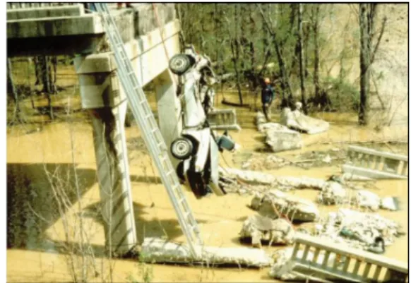
Bridges are perhaps the most critical targets of underwater inspection from a safety standpoint. According to the U.S. Department of Transportation, 83% of the 600,000 bridges in the United States span waterways. Many of these bridges have support structures underwater, which wear quickly due to scouring by abrasive suspended particles carried by the currents or “prop wash” from pass-ing ships. Floodpass-ing carries debris which pile up against bridge supports, and washes away supporting soil beneath bridge anchors. Due to their proximity to motor vehicles and other human infrastructure, bridges are often submerged in chemical-laden polluted water, increasing the rate of corrosion [13]. Given these factors, it may come as no surprise that most bridge collapses are due to failure of submerged elements [1]. A string of high-profile bridge collapses in the mid

(16)

(a) Schoharie Creek bridge collapse, Fort Hunter, NY, 1987 (USGS)

(b) US51 bridge collapse, Hatchie River, TN, 1989 (USDOT)

Figure 1-3: The Schoharie Creek bridge (a) and the Hatchie River bridge (b) both collapsed due to excessive scour of the support pier foundations, leading the U.S. Department of Transportation to develop improved guidelines for regular bridge in-spection.

1980s led the U.S. Department of Transportation to create a set of standards for bridge inspection, including the planning, executing, and documenting the inspection of underwater inspection tasks [13].

1.1.2 Types of inspection

Which, if any, of these inspections could be performed by an AUV? Some, like ul-trasound hull thickness measurements, require specialized tools. Others, like flooded member testing, can be done from the surface. AUVs would be most suited for tasks that can be done with standard underwater cameras and sonars. Within these tasks, there are widely varying requirements for coverage and precision. Inspecting welds or microfractures requires close-up imagery with millimeter-scale resolution, but detect-ing fallen debris, bent support beams, or unwanted attachments (bio, mines) could feasibly be done with centimeter or decimeter scale sonar.

The USDOT Federal Highway Administration defines the following types of in-spection for bridges [13]:

Type I The visual, tactile inspection, also called a “swim-by” inspection, should be detailed enough to detect “obvious damage or deterioration.” The target should

(17)

be examined visually or, if visibility is poor, by touch. Generally every element of the structure receives a full level I inspection.

Type II Thedetailed inspection with partial cleaningconsists of removing biofouling in small patches to obtain detailed estimates of corrosion and deformation. Generally, a randomized representative subset of structural elements will receive a level II inspection.

Type III If the type II inspection reveals structural issues, it is followed up with a highly detailed inspection, usually involving non-destructive or partially-destructive testing.

These inspection tiers have been also adopted for harbors [43] and open water oil platforms [71].

We hope to automate level 1 surveys using a two-stage inspection process. First, the vehicle performs a long-range sonar inspection, or “safe distance survey,” to con-struct a rough map of the inspection target. The safe distance survey consists of a simple lawnmower pattern at sufficient distance to avoid collision with the object, generally between 5 and 10 meters. Using the model created from the safe distance survey, the vehicle plans a trajectory for a detailed inspection at 1 to 5 meter range. The detailed inspection can be designed to use a camera, sonar, or both.

1.2 Partially structured environments

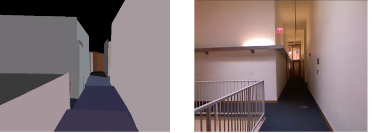
In general, robots tend to operate near humans and human-created infrastructure. As a result, most environments that a robot must map and navigate will exhibit some sort of regular structure. Using prior knowledge of the environments structure can greatly simplify the tasks of mapping and navigation. The most basic example of this is 2D laser mapping by indoor wheeled robots [85], which operates under the assumption that floors are horizontal and walls are vertical. This assumption reduces the complexity of mapping from 3D/6DOF to 2D/3DOF. Work in planar mapping attempts to detect flat surfaces in point cloud data, and use the extracted planes to

(18)

Figure 1-4: Human-occupied environments have predictable features, such as walls and floors, which can be used to improve localization and mapping. The higher-level representation is generally more compact, and produces more accurate map estimates for a given amount of sensor data. (Source: Hordur Johannsson [37], used with permission).

generate constraints on vehicle position (see Section 5.1.1 for examples and analysis of some of these techniques). At a higher level, 3D objects can serve as landmarks for mapping. Salas-Moreno et al. present a system for mapping based on object detection in 3D point clouds [82].

There are several advantages to mapping based on higher-level landmarks. First, these high level features can produce fuller maps from limited sensor data, or data with less overlap. They require only enough data to detect the object, such as one view of a chair, to reconstruct the full object in the final map. Second, in addition to operating on a lower quantity of data, these techniques may be able to operate on lower quality data. While a wall scanned with a noisy sensor will require the averaging of many measurements to produce a smooth result, a smooth plane could be extracted from the noisy data. Third, they can produce a more compact repre-sentation of the environment, by reducing redundancy (e.g. tracking chair locations rather than full point clouds for each chair) or replacing dense point cloud data with parametric surfaces. Finally, these techniques may produce more “meaningful” maps if the features are well-matched to the usage of the final map. For example, a map used for ray-tracing will be more useful if closed surfaces are explicitly represented, instead of being interpolated from an unorganized point cloud.

(19)

However, it is not immediately apparent what structure can be leveraged in an un-derwater environment. They are not occupied by humans, so we can’t track features based on their human a↵ordances, such as walls or chairs. However, we can make some assumptions based on what the infrastructure is used for. First, because these structures are submerged, they are generally composed of smooth surfaces. Many un-derwater structures are designed to be hydrodynamic, and therefore exhibit relatively slow changes in gradient. Even structures for which hydrodynamics is not a consid-eration are usually built with smooth, solid faces unless the functionality requires otherwise. Second, most of these structures are watertight, for the somewhat obvious reason that they are specifically designed to be a barrier against water. Third, we can make general assumptions based on human design patterns: anthropogenic structures are often built using straight lines and flat faces, unless the application specifically requires otherwise (such as a dam curved inward to increase strength).

In addition to geometric structure, underwater infrastructure may exhibit dis-tinctive visual features. Components in o↵shore infrastructure must be labeled for inspection and maintenance, for example with a serial number, part ID, or bar code [3]. Many currently deployed tags are high-contrast corrosion-resistant labels (e.g. http://www.aquasign.com), which could be recognized by a camera and used as a high accuracy zero-drift waypoint for navigation and mapping. Additionally, the cost of installing robot-specific markers, such as visual fiducial markers, is small compared to the cost of regular manual inspection .

We want to design a system to take advantage of both geometric and visual regularity in the environment.

1.3 Requirements

Full coverageof the target structure is a requirement of most level I inspection tasks. This entails requirements for both planning and navigation. We use existing tech-niques from coverage planning to generate a trajectory that covers the full structure. In many situations, it is sufficient for the vehicle to have an accurate estimate of its

(20)

current position only. In this case, filtering solutions such as EKF or particle filtering, which can run efficiently in real time, are good solutions. However, inspection tasks require that we have an accurate estimate of the entire vehicle trajectory, not just the current pose. This allows us to verify that the entire inspection target has been covered.

We also requires that the robot be able to localize itself to accurately follow the trajectory. Because it is important that the vehicle follow the inspection path as closely as possible, we require these trajectory estimates online, rather than in post-processing, as is common with many autonomous underwater operations. Therefore, our system must be designed and implemented for computational efficiency, to be able to provide real-time position estimates on the low-power computers typical of AUVs.

Because many inspection tasks are in water with poor visibility, we require that the vehicle be able to use multiple sensors. Vehicles are commonly equipped with a camera and sonar, and it is desirable to have the ability to generate loop closures from either sensor.

1.4 Contributions

We have developed an algorithm for underwater SLAM in partially structured envi-ronments, using sonar and camera data. Our main contributions are:

1. A denoising and parametric surface modeling technique for improved alignment of sonar submaps.

2. A technique for tracking sonar submaps and generating pose-relative constraints based on submap alignment.

3. A framework for visual and acoustic SLAM using factor graphs.

4. Experiments with localization and mapping using sonar and camera data in a swimming pool and on the hull of a decommissioned aircraft carrier.

(21)

The remainder of this thesis is structured as follows:

Chapter 2 introduces the vehicle and the specifics of our underwater inspection task.

Chapter 3 introduces our framework for planning inspection tasks, integrating sen-sor data, and constructing and optimizing a factor graph to estimate vehicle trajectory.

Chapter 4 describes our technique for generating loop closures from submap align-ment, including the creation, smoothing, and alignment of submaps from noisy sonar data, and presents evaluation from an inspection task on theUSS Saratoga, a decomissioned aircraft carrier.

Chapter 5 describes out technique for generating loop closures from structured ele-ments, including detection of visual fiducial markers from camera imagery and extraction of planar segments from sonar submaps, and presents experimental results from an indoor structured environment.

(22)

(23)

Chapter 2 Inspection of Partially Structured

Underwater Environments

This chapter presents the challenges in underwater inspection and existing solutions that have informed this work.

2.1 Challenges in underwater navigation

A fundamental challenge of underwater operations is the lack of global positioning information, because water quickly blocks electromagnetic radiation, from visible light through the frequencies used by satellite-based GPS. As a result, many underwater navigation techniques are based on highly accurate dead reckoning. Reduced visibility, strong currents, and the relative lack of distinctive visual or topographical features further complicate underwater localization. However, sound travels rapidly and with low attenuation due to water’s relatively high ratio of sti↵ness (bulk modulus) to density. As a result, acoustic sensors provide some of the best tools for underwater localization.

The sensors commonly used in underwater operations are:

Control inputs The simplest form of navigation is to simply assume an ideal vehicle model that moves exactly as commanded. For land robots with wheel encoders, this can be a fairly accurate solution if there is no wheel slip. For underwater

(24)

applications, modeling the relationship between control inputs (such as propeller RPMs) and vehicle motion is more complicated, due to highly nonlinear thruster response and hydrodynamic forces such as drag.

Magnetic compass One of the oldest navigation sensors is still one of the most useful for underwater navigation. Compasses provide an absolute heading ref-erence, which can be combined with an estimate of vehicle velocity or distance traveled to produce a position estimate. A typical compass used in underwater operations provides heading estimates at 1-2Hz with an accuracy of 1 10 [97]. Unfortunately, magnetic compasses are subject to magnetic interference near large metal structures, making them unsuitable for close inspection of most marine infrastructure.

Pressure sensor A depth gauge is used almost universally in underwater applica-tions. Because water density changes with temperature and salinity, the most accurate systems combine a reading from a pressure sensor with a measured or predetermined profile of temperature and salinity in the water column [19]. A properly calibrated pressure sensor produces zero-drift measurements at 1Hz with accuracy on the order of .01% [97].

Gyroscope A gyroscope provides an orientation estimate by measuring rotation using the conservation of angular momentum. The simplest form is a rotat-ing weighted disc, which resists rotation in any direction other than the spin axis. Combining measurements from multiple orthogonal gyroscopes allows full 3DOF orientation estimate. The most common gyroscope in modern applica-tions is a Micro Electro-Mechanical System (MEMS) gyroscope, which uses a the vibration of a mechanical element to measure angular velocity. MEMS gy-roscopes are small enough to fit onto an integrated circuit, and are commonly found in cell phones and other consumer electronics. In aerospace, defense, and underwater applications, more expensive and accurate units are used, based on acceleration-induced phase di↵erence between two light beams traveling in opposite directions around a loop. The two most common implementations

(25)

are fiber optic gyroscopes (FOG) and ring laser gyroscopes (RLG). These gyro-scopes are accurate enough to detect the rotation of the earth, and can therefore be used for absolute heading reference using gyrocompassing. Gyrocompassing has the added benefit of finding true north, rather than magnetic north. Gyroscopes tend to exhibit low “jitter” but high drift. A MEMS gyrocompass exhibits precision of under one degree and drift on the order of 10 /hr [97], whereas a high quality RLG has precision of hundredths of a degree and drift of less than.5 /hr [96].

Accelerometer Accelerometers measure linear acceleration, which can be integrated once to find linear velocity, or twice to find position. An array of three or-thogonal accelerometers is commonly used to produce 3D position and velocity estimates. Because position is calculated as a double integral, small amounts of noise in the initial acceleration measurement will be amplified and cause large amounts of drift in the position estimate. An uncalibrated stationary ac-celerometer will measure an acceleration of 9.8 m/s2 in the direction opposite earth’s gravity. Measurement of earth-relative position therefore requires ac-curate estimates of the direction and magnitude of earth’s gravity, which are subtracted out of the estimated acceleration.

Accelerometers are commonly combined with gyroscopes in anInertial Measure-ment Unit, or IMU. The full system of estimating position and heading using an IMU is called an Inertial Navigation System (INS) or Attitude and Heading Reference System (AHRS). The heading estimate produced by an AHRS/INS has been shown to be roughly twice as accurate as the estimate produced by an uncorrected gyrocompass [28]. However, the position estimate of these units exhibits drift on the order of several kilometers per hour [52].

Doppler Velocity Log A Doppler Velocity Log, or DVL, uses Doppler shift in acoustic backscatter to measure the relative velocity of the water column or seafloor. DVL units commonly have four highly directional beams measuring the intensity and Doppler shift along a series of range bins. AUV applications

(26)

typically use a high frequency (1200 kHz) unit with a range of 30m [97], mounted on the bottom of the vehicle and pointed at the seafloor. For each beam, the bin with the highest amplitude can be used to estimate the distance to the seafloor, and the Doppler shift of this bin can be used to find the component of seafloor-relative sensor velocity along the vector of the beam. Combining the velocity components from at least three beams gives an estimate of the full 3DOF sensor velocity relative to the seafloor; four beams are typically used. A DVL measuring only the water velocity is called an Acoustic Doppler Current Profiler, or ADCP, and is commonly used to estimate currents for scientific research. The current-measuring ability of the DVL/ADCP has also been been used on an AUV to estimate water current and vehicle position during the vehicle’s descent phase, before bottom lock is acquired [84].

A typical navigation-grade 1200 kHz DVL has zero-mean noise with a standard deviation of .2% of measured velocity [97]. Position estimates generated by integrating velocity will therefore drift in a random walk, with the magnitude of position error dependent on vehicle velocity and attitude. Because each beam provides a range to the seafloor, the DVL can also be used as a zero-drift acoustic altimeter.

Acoustic Ranging It is often desirable to find the global position of the vehicle, commonly accomplished by acoustic ranging to objects at known positions. One such system is Long Baseline (LBL) acoustic positioning, in which a network of transponders is deployed around the vehicle’s operating area. The vehicle can triangulate its position using ranges from three transponders; additional transponders are generally deployed to increase redundancy and accuracy [29]. To provide absolute position reference, the geo-referenced position of each bea-con must be accurately calibrated. In many applications, local position is suf-ficient, which requires only the relative positions of the transponders. Once installed, the transponder array can operate for long periods of time and pro-vide zero-drift navigation for multiple vehicles in the work area. Therefore, LBL

(27)

is commonly used as sites of long term research and monitoring.

A typical long-range LBL unit operates at 12kHz, has a range of up to 10km, and zero-mean range-dependent position error up to 10m [34]. For short ranges, a 300kHz LBL array can provide centimeter-precision positioning accuracy up to about 100m [97]. LBL error is heavily dependent on the calibration error of the beacon positions. Additionally, generating accurate range information from round trip time requires knowledge of the sound speed profile of the water, which is primarily governed by temperature and salinity. In shallow areas, particularly the first tens of meters of the ocean water column, temperature and salinity change rapidly with depth, and may also vary over short time periods due to wave action. LBL is also susceptible to multipath interference due to reflections, and is therefore less accurate in shallow environments, near the surface, or under ice [52].

When it is impractical to install an LBL array, a ship-mounted system, combined with the ship’s GPS, can provide accurate globally referenced position. Short Baseline (SBL) localization uses a transponder array mounted along the length of the ship, or hung over the sides. Position is then triangulated as in an LBL system. More commonly used is Ultrashort Baseline, or USBL, in which multiple transducers are mounted in a single transceiver unit. Rather than triangulation used in LBL and SBL systems, USBL measures range and bearing from the transceiver. Range is detected using round trip time from the ship mounted transceiver, as with a single LBL beacon. Bearing is calculated using the phase di↵erence between the transducers.

Ship-mounted systems are more quickly deployed than LBL units, and can provide a similar level of accuracy when the target vehicle is in a narrow working window below the ship. USBL error is dominated by error in the measured bearing, which, although typically under 1 , leads to increasingxyz localization error with increasing distance [83] [89]. Because they require a ship to follow the vehicle, they can be inconvenient for long term deployments. As with all

(28)

acoustic ranging systems, USBL is susceptible to errors in the estimated sound speed profile.

Other environmental sensors Other sensors commonly mounted on AUVs in-clude cameras and sonar units. These can provide relative position estimation by tracking objects between subsequent frames, and estimating vehicle motion using an assumption of stationary objects. This visual odometry requires the ability to extract accurate features from camera or sonar images. SIFT [55] [54] are similar gradient-based features are commonly used in camera imagery. The Normal Distribution Transform has been used to align frames from an imaging sonar to aid in AUV navigation [44].

However, as with other incremental measurements, visual and acoustic odom-etry do not correct for long term navigation drift. When a prior map is avail-able, features from the map can be used to provide zero-drift global position estimates.

These odometry and localization techniques are not limited to cameras and sonar. Other environmental sensors mounted that have been used on AUVs include sheet lasers [75], fluorometers [15], mass spectrometers [36], optical backscatter sensors [100], and magnetometers [88]. If a prior map of sufficient resolution is available, these environmental sensors can be used to navigate within the map.

2.2 Approaches to underwater navigation

The sensors described above are rarely used in isolation; more commonly, they are combined in a multi-sensor estimation framework to provide an improved position estimate. This is particularly beneficial when the sensors have di↵erent noise char-acteristics. A comprehensive overview of AUV navigation techniques can be found in [52]; a short summary is below.

(29)

us-ing local measurements projected from a known global position. Any of the relative sensors described above – command inputs, accelerometer, gyroscope, visual odometry – could be considered a dead reckoning solution when used in isolation. In general, combining multiple sensors with uncorrelated noise provides greater accuracy than any individual sensor. In underwater appli-cations, the most common dead reckoning configuration is a DVL and IMU supplemented by a compass and depth sensor. These sensor measurements are generally combined in a filtering framework based on the Kalman filter [42]. Dead reckoning may also be used with other relative position measurements, such as visual odometry or acoustic scan-matching. A well-tuned system using scan-matching from an imaging sonar has been shown to have accuracy on the order of .02% of distance traveled [66].

By definition, dead reckoning lacks an absolute position reference to correct ac-cumulated error. Therefore, the error in dead reckoning estimates will inevitably tend to increase over time.

Acoustic Beacons + Dead Reckoning To correct accumulated error in the dead reckoning position estimate, it is common to combine the DVL+IMU system with a zero-drift acoustic positioning system such as LBL or USBL. This lever-ages the complementary noise characteristics of dead reckoning, which has low jitter and high drift, and LBL/USBL, which has high jitter and low drift, to produce a significantly improved position estimate. For real time operation, the time-of-flight measurements can be added directly to the filtering framework, with the low-jitter dead reckoning estimate used for outlier rejection on the acoustic position estimates [91]. If navigation is corrected in post-processing, the time domain error characteristics of each sensor can be removed in the frequency domain, and the sensors combined with a complementary filter [97].

Prior Map When a prior map is available, it is possible to localize within this map using available sensors. Gravitational [52], magnetic [28], and bathymetric [38] data have all been used for underwater localization. The localization accuracy

(30)

is limited by the spatial resolution of the signal. For example, bathymetric localization will be inaccurate on a flat, featureless bottom. This technique also requires creating a prior map of sufficient resolution, and updating the map to reflect changes in the environment.

SLAM When a prior map is not available, it is possible to navigate relative to natural landmarks using SLAM. See Section 2.4.1 for an overview of prior work in this area.

Of these techniques, only SLAM meets our requirements for high-accuracy posi-tioning near underwater infrastructure. SLAM is well-suited for underwater inspec-tions because it is more accurate than dead reckoning and requires less infrastructure than global acoustic positioning. Additionally, many inspection environments are ill-suited to LBL/USBL acoustic positioning due to multipath interference and the difficulty of installing and maintaining infrastructure in a crowded harbor environ-ment.

2.3 Inspection with the HAUV

The MIT-Bluefin Hovering AUV (HAUV) is designed for shallow-water inspection tasks in complex environments. These inspections are generally performed by divers or ROVs, and would be difficult if not impossible to accomplish with most current-generating AUVs. To create an AUV for complex inspection posed challenges in vehicle design, visual-acoustic mapping, and coverage planning. Prior work of our collaborators in each of these areas is presented below.

2.3.1 Vehicle design

The physical design of most current-generation AUVs is designed primarily for effi-cient bathymetric mapping and photo surveys, which have vastly di↵erent require-ments than the inspection of underwater infrastructure. In particular, complex

(31)

in-Figure 2-1: Bluefin Hovering Autonomous Underwater Vehicle with Soundmetrics DIDSON sonar.

spection requires greater maneuverability and sensor coverage than provided by the current generation of AUVs.

Maneuverability Most AUVs designed for long-range or deep water operations have a torpedo shape to reduce hydrodynamic drag, thereby reducing the volume and weight of the propulsion and battery systems. Cornering is accomplished using actuated fins, or by changing the angle of the main rear thruster. Vertical motion is primarily accomplished with buoyancy control, with small changes possible through steering. As a result, tight cornering and arbitrary depth changes are difficult with this form factor. Additionally, the torpedo shape is relatively unstable in the roll direction. Roll stability is particularly important for multibeam mapping operations, where small roll errors translate into large bathymetry errors on the outer edges of the sonar swath. “Sail” shape and dual-hull AUVs increase roll stability by increasing the distance between center of buoyancy and center of mass. The use of di↵erential drive allows for tighter cornering, which allows a tighter spacing between track lines in a bathymetric survey.

On the other end of the spectrum, the common “box” form factor of ROVs increases maneuverability and stability at the expense of increased power and thrust requirements due to hydrodynamic drag. These almost universally

(32)

em-ploy di↵erential drive, with thrusters positioned to allow full control of position and heading.

The HAUV was built with the maneuverability of an ROV, with five thrusters allowing arbitrary motion in x, y, z, and heading. The negatively buoyant bat-tery and pressure housing are low in the vehicle, and the flotation is high, providing passive pitch and roll stabilization. Additionally, the placement of the two vertical thrusters allows active correction of vehicle pitch to maintain a level platform for mapping.

Sensor Coverage AUVs designed for mapping typically have downward-facing bathy-metric mapping sonars, forward-looking imaging sonars, or sidescan sonars mounted on the underside of the vehicle. Some vehicles have been modified or designed with upward-facing sonar and DVL units for mapping the under-side of sea ice [48] [12].

The HAUV carries a DIDSON multibeam sonar, detailed in Section 4.1.1, as well as two underwater cameras and a blue-green LED lighting array. The DIDSON can be used as either a narrow-beam mapping sonar or a wide-beam imaging sonar.

Complex inspection requires the ability to look up, down, or forward, often over the course of a single inspection. To this end, the HAUV was designed with a rotating instrument basket to hold the DVL, sonar, and camera. This allows the DVL to be aimed downward in the traditional bottom lock configuration for seafloor-relative positioning, or to be aimed at the inspection target for target-relative positioning.

The sonar is mounted on a 90 tilt mount within the front basket. It can be held at a fixed position or it can be swept in an arc independent of the DVL. The fixed position is generally used for imaging sonar or standard lawnmower surveys with profiling sonar, while the sweep is used for close-range inspection with profiling sonar.

(33)

For navigation, the HAUV is equipped with the standard sensor package of DVL, IMU, and pressure sensor. The IMU is a Honeywell HG1700 Ring Laser Gyro, which gives heading estimates with a bias of 2 /hr, and zero-drift pitch and roll measure-ments with an accuracy of 0.1 /hr. The DVL is a RDI Workhorse operating at 1200 kHz, with an accuracy of .2% of vehicle velocity. The pressure sensor has an accuracy of .01% with zero bias. [94] A compass is not used because the vehicle is expected to operate near large metal structures such as ship hulls, which create magnetic inter-ference.

The vehicle’s main processor performs sensor fusion, status monitoring, and waypoint-based position control in the dead reckoning frame. The estimated position, along the sensor data, is passed o↵ to a second computer through a backseat driver inter-face. The backseat computer can either be onboard or remotely attached over the fiber-optic tether.

2.3.2 Non-complex area SLAM

Our collaborators have created a SLAM system for surveying the non-complex areas of the hull, which can be covered with a standard lawnmower survey. For the non-complex areas, the sonar, DVL, and underwater camera are continually aimed at the hull using the rotating front basket. The DIDSON is operated in imaging mode, with a low grazing angle, aimed laterally across the hull. At each time step, the vehicle’s uncertainty is compared to the cost of reducing uncertainty by revisiting a previous location for a loop closure in sonar or camera data. If the gain of returning for a loop closure is greater than the cost, the vehicle pauses its survey and returns to the previous location; this is a variant of active SLAM which the authors refer to as Perception Driven Navigation [46] [45]. The expected information gain from a visual loop closure is estimated using visual saliency [47], which roughly corresponds to the “distinctiveness” of an area, and therefore the probability of generating a reliable loop closure from visual features. Using a piecewise planar assumption, they track features in the imaging sonar, and align them using the Normal Distribution Transform. They optimize the vehicle trajectory and plane locations in real-time using an incremental

(34)

factor graph solver [65].

2.3.3 Coverage planning

The remainder of the hull, including the propellers, driveshafts, and rudders, we refer to as the complex area. The non-complex areas can be completely surveyed using a standard trackline survey, assuming navigation drift is accounted for. This can be done either by following a preplanned survey and correcting navigation through SLAM, or by adaptively replanning based on updated position estimates [70]. How-ever, fully surveying the complex areas is non-trivial even in the case of perfect navi-gation. The survey pattern must inspect each surface, taking into account occlusion, and must follow a collision-free path to do so. The problem of generating a trajectory that ensures full coverage of the structure is known as coverage planning, and con-sists of multiple sub-problems, primarily generating subsets of viewpoints that cover the entire structure, selecting the best subset, and planning a collision-free trajectory between the selected waypoints. The optimal solution can only be found through ex-haustive search, which is computationally infeasible. Our colleagues have developed a sampling-based coverage planning algorithm [20] [21] using redundant roadmaps to efficiently generate multiple full-coverage waypoint sets and select the lowest-cost subset of waypoints that guarantees full coverage. They have also developed an iter-ative smoothing technique [22] to improve the resultant trajectories without loss of coverage.

This prior work has assumed perfect localization of the vehicle. These algorithms could potentially be modified to tolerate bounded navigation error in both collision avoidance, e.g. by inflating the vehicle size by the amount of expected position error, and sensor coverage, e.g. by reducing the field-of-view of the simulated sensor during the coverage planning waypoint generation. However, even a small amount of heading error can quickly lead to position error much larger than the vehicle, or even the sonar field of view, meaning that these ad-hoc solutions would quickly become intractable. Full-coverage surveys of complex area require a navigation solution to correct accumulated drift in the dead reckoning estimate. In non-complex areas, this is

(35)

provided by a SLAM system assuming local planarity, however this assumption does not hold for complex areas. There is a large body of relevant prior work in underwater mapping, 3D SLAM, and surface modeling, however, we did not find a system that met our specific requirements for close-range complex-area inspection. We therefore created a SLAM system for mapping these complex areas that is: 1.) efficient enough for online operation, 2.) able to utilize both visual and acoustic loop closures, 3.) capable of using environmental structure in the form of planes extracted from sonar point clouds, 4.) robust to sonar error.

2.4 Existing Solutions

This paper builds upon a large body of prior research in underwater simultaneous localization and mapping (SLAM), 3D mapping, and dense point cloud alignment.

2.4.1 SLAM

The goal of SLAM is to correct for drift in the vehicle’s dead reckoning by using repeated observations of static landmarks in the environment. There are two broad families of approaches: filtering and smoothing. Both approaches generally assume Gaussian process and measurement error models.

Filtering approaches track the robot’s current pose by incrementally adding dead reckoning and loop closure constraints. Because constraints are added incrementally, this approach is naturally suited to real-time operation. The extended information filter (EIF) [87], in which the normal distribution is parameterized in terms of its information vector and information matrix rather than its mean and covariance, has a sparse structure which enables efficient computation.

Barkby et al. [7] used a particle filter along with a bathymetric sonar to produce a 2.5D map of the seafloor in real time. The extended Kalman filter (EKF) has been applied to imaging sonar data [74], and forward-looking sonar [26] collected by AUVs. Walter et al. [93] used a filtering approach to survey an underwater structure using features manually extracted from an imaging sonar.

(36)

A disadvantage of filtering approaches is that they estimate only the current ve-hicle pose. Because information from loop closure constraints is not back-propagated to correct previous pose estimates, these approaches do not provide an accurate es-timate of the entire vehicle trajectory. This is particularly problematic when adding constraints from large loop closures, which produces discontinuities in the estimated vehicle path.

Smoothing approaches also include all past poses into the optimization. Exploiting the fact that the information matrix is exactly sparse in view-based SLAM, Eustice et al. [23] applied the information filtering approach to camera data from the RMS Titanic, producing a 6-DOF trajectory estimate. Dellaert and Kaess [17] formulate the SLAM problem as a bipartite factor graph, and provide an efficient solution by smoothing and mapping (SAM). Incremental smoothing and mapping (iSAM) [41] incrementalizes the matrix factorization to efficiently integrate new constraints without refactoring the information matrix.

In the underwater domain, pose graphs have been shown to produce more consis-tent maps due to their ability to correct prior navigation error and relinearize around the corrected trajectory. Beall et al. [8] used an o✏ine pose-graph based smoothing approach to estimate a full 6-DOF trajectory in a large-scale underwater photo sur-vey. Kunz and Singh [49] applied o✏ine pose graph optimization to visual and sonar data. Pose graphs have been used for real-time mapping of a locally planar complex structures such as ship hulls [32].

In bathymetric and photomosaicing applications, a 2.5-dimensional representation of the environment (depth map) is sufficient, but complex environments require a full 3D representation. Fairfield et al. [24] use evidence grids inside a particle filter to perform real-time 3D mapping of a sinkhole with an imaging sonar.

2.4.2 Submap SLAM

Submap alignment requires generation of loop closure constraints, which, in visual SLAM, are commonly derived using viewpoint-invariant visual features such as SIFT. However, bathymetric and profiling sonars generally do not produce easily

(37)

iden-tifiable viewpoint-invariant features. If the vehicle dead reckoning is accurate over short time periods, as is the case with most IMU and DVL based systems, the sonar data can be aggregated into “submaps” for improved matching.

For terrestrial mapping, point cloud-based approaches [63] [11], which use iterative closest point (ICP) to align submaps, have been applied to depth camera and scanning laser data.

In the underwater domain, McVicker et al. [57] created 2D maps of flooded archae-ological sites using a small ROV equipped with a 360-degree scanning sonar. Because the ROV does not have an inertial sensor to produce dead reckoning estimates, sonar data was collected while the vehicle was stationary. The authors note that standard scan-matching techniques developed for laser data perform poorly when applied to noisy sonar data. They instead develop a denoising and alignment pipeline based on particle filter localization [86].

Roman and Singh have used submap alignment for bathymetric (2.5D) mapping with an AUV and multibeam sonar. They use cross-correlation [77] and ICP [76] to provide constraints for EKF SLAM. These are perhaps the most closely related to the work presented here. However, their filtering approach does not optimize the full vehicle trajectory, and is susceptible to linearization errors when initial position estimates deviate from ground truth.

(38)

(39)

Chapter 3 A Framework for Visual-Acoustic

Factor Graph SLAM

This chapter describes our framework for autonomous ship hull inspection using fac-tor graph SLAM. The core of our mapping framework is iSAM [41], which allows efficient online optimization for factor graph SLAM. Our system runs in real time during field operations, and at approximately 4x speedup on a standard consumer laptop. The system consists of various modules for pre-processing sensor data, storing and aligning submaps, and constructing and optimizing the factor graph. The sen-sor front-end modules are decoupled from the mapping back-end using Lightweight Communications and Marshalling (LCM) [33], a low-overhead publish-and-subscribe architecture for network communications. This decoupling enforces a standard inter-face and allows us to easily substitute or add new sensors.

3.1 Problem formulation

We formulate poses and constraints into a factor graph, a bipartite graph in which nodes represent vehicle and landmark poses, and factors represent constraints on vehicle and landmark poses. Our factor graph will have three types of nodes: vehicle poses X, landmark posesL, and planes E.

(40)

Dead Reckoning Camera Image Rectification AprilTag Detection Sonar iSAM Submap Formation Plane Catalog Plane Alignment Submap Catalog Submap Alignment ˆ x_t ppol_t,₀_..₉₆ st st Proposal ˆ xi,ei$ˆxj,ej Proposal ˆ xi,si$ˆxj,sj Observation zk,⌃k Observation (ei, j),⌃i Constraint cij,⌃ij ˆ xt ,⌃t ˆ x

Figure 3-1: Architecture of visual-acoustic SLAM with planar constraints

coordinates as xt = [x, y, z, ,✓, ], using standard Euler angles for yaw, pitch, and roll. 1 _{The choice of origin does not a↵ect our position estimates, although due to} Euler angle singularities it is more convenient to choose a coordinate system that avoids high pitch and roll angles. We initialize x, y, z,and heading to 0 at the first robot pose, with pitch ✓ and roll initialized relative to gravity using the estimate produced by the IMU.

We refer to the estimated vehicle poses as ˆxt to distinguish them from ground-truth poses xt.

We model the vehicle and landmark positions as a joint probability distribution P(X, C, Z, L, E, F, U), where:

1_{Although we use Euler angles in formulating poses and constraints, they are represented}

(41)

X represents vehicle positions.

C represents constraints between nonconsecutive vehicle poses. Z represents 6DOF landmark positions.

L represents constraints between vehicle positions and 6DOF landmark positions. D represents planar landmark positions.

E represents constraints between vehicle poses and planar landmark positions. U represents constraints between consecutive vehicle poses from dead reckoning

es-timates.

We can directly write the joint probability as:

We find the maximum a posteriori(MAP) estimate using the standard technique of minimizing the negative log probability:

ˆ X,Z,ˆ Dˆ = arg max X,Z,D P(C, L, E, U|X, Z, D)P(X, Z, D) = arg max X,Z,D P(X, C, Z, L, D, E, U) = arg min X,Z,D logP(X, C, Z, L, D, E, U) (3.2)

(42)

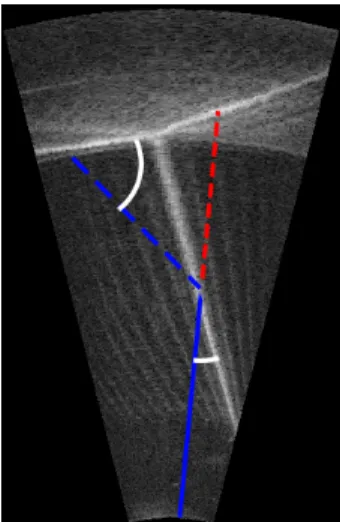
Figure 3-2: Coordinate system of the HAUV [37]

3.2 SLAM server

The role of the SLAM server is to asynchronously collect constraints from various sensors, combine them into a factor graph, and provide updated pose, landmark, and uncertainty estimates to other vehicle services. We use iSAM [41] to formulate and solve the factor graph.

Constraints come from a variety of sensors with varying time delays due to data transmission and post-processing. Full-resolution camera images are large, and may arrive several seconds late due to network congestion. Constraints from camera data may be further delayed due to image processing. Constraints based on submap align-ment may arrive late due to the time required to denoise and smooth the sonar data. Our system adds target observations and pose to pose loop closures as they arrive, creating a new node and initializing it with the dead reckoning estimate.

3.2.1 Types of constraints

In general, constraints in factor graph SLAM take three forms: absolute, pose to pose, and pose to landmark. Absolute constraints are unary– they operate on a single node. Pose to pose constraints and post to landmark constraints are binary, representing a relative transformation between two nodes. Our particular implementation uses multiple types of absolute and relative constraints, described below.

(43)

Absolute constraints Absolute constraints are constraints on a single pose relative to the world coordinate frame. We initialize our robot position with a weak absolute constraint at the origin. We also use absolute constraints for the depth, pitch, and roll portions of the robot position. See Section 3.2.2 for details.

“Odometry” We refer to constraints between consecutive vehicle poses as odometry constraints, borrowing terminology from wheeled robot mapping. We use x_t

to refer to the ground truth vehicle motion between timet 1 and time t, such that xt = xt 1 xt . We use ˆxt to refer to the dead reckoning estimate of x_t produced by the IMU. Our dead reckoning constraints between consecutive poses are thereforexˆt=ˆxt 1 ˆxt .

Pose to pose loop closures These are loop closures formulated as constraints be-tween two non-consecutive poses, generated from submap alignment. In our implementation, pose to pose constraints from submap alignment arecij, which

represent the relative transform between anchor posesxiandxj . See Section 4.6 for details.

6DOF landmark observations Another form of loop closure is observation of a previously observed landmark. We denote the set of landmarks L={lj}, with j ₂0. . . N, where lj = [x, y, z, ,✓, ] is the position of landmarkj. Landmark observations are Z = {zk} With 6DOF constraints zk = [x, y, z, ,✓, ] rep-resenting the relative position of the landmark from the robot pose . We use 6DOF landmark constraints for observations of our visual fiducial markers; see Section 5.2 for details.

Planar landmark observations Loop closures can also be generated by observa-tion of a previously observed plane. We formulate planar constraintsE in terms of the plane equation (unit normal and distance to origin) in the local vehicle frame. See sec 5.1 for details.

(44)

3.2.2 Dead reckoning and partial constraints

Dead reckoning loosely refers to vehicle-relative motion estimates from a moving platform. “Odometry” is often used to refer to dead reckoning solutions, e.g. visual odometry, and as a result, the words are often used interchangeably. The canonical example is wheel odometry, either measuring the rotation of the wheels using a rotary encoder, or, in the case of the Soviet Lunokhod rovers, an extra wheel acting as a dedicated odometer.

However, many dead reckoning systems combine absolute and relative measure-ments into the dead reckoning estimate (see Sec. 2.2 for examples of common ap-proaches in the underwater domain). In our case, constraints on depth z come from a pressure sensor, which provides an absolute measurement of vehicle depth. Con-straints on pitch and roll come from the IMU’s accelerometers, which provide and absolute measurement of the vehicle’s orientated with respect to gravity. x, y, and heading are relative constraints, computed by combining IMU and DVL estimates, and are formulated as binary partial factors between consecutive poses. In a factor graph, dead reckoning combining relative and absolute measurements can be formu-lated as two or more partial constraints. Partial constraints represent measurements with fewer degrees of freedom than the full robot state. In our case, depth, pitch, and roll are formulated as absolute partial constraints, unary factors applied only to those components of the robot state. The other state variables estimated by the IMU and DVL are x, y, and heading, which are formulated as relative partial constraints, binary factors constraining the remaining degrees of freedom between poses.

Note that the degrees of freedom in a partial constraint do not necessarily corre-spond directly to the constrained node’s state variables. A classic example of partial constraints is measurement of a point feature, such as SIFT, in a 2D camera image. A SIFT feature is a point in R3_{. Using knowledge of the camera’s focal length and} principal point, the feature’s bearing (azimuth and altitude angles) can be recovered from its position in the 2D image, but its range cannot. If we wish to formulate the relative partial constraint between the camera and the feature in Cartesian

(45)

co-ordinates, we cannot do so by simply removing some state variables as in odometry estimates. Instead, we would have to define a factor in terms of azimuth and eleva-tion, and evaluate the cost of a proposed feature location (x, y, z) by computing its azimuth and and elevation relative to the camera. Another example of partial con-straints using the full state variables can be seen in the planar concon-straints described in Section 5.1.

If we tried to optimize the least-squares problem representing the position of this landmark, we would find that it does not have a unique solution. Therefore, unless special provisions are made to handle non-unique solutions within the least squares solver (e.g. choosing an arbitrary point in the unconstrained dimensions), we must always ensure that the robot and landmark poses are fully constrained; that is, that there is a unique solution when all factors are considered. We therefore add our absolute and relative constraints simultaneously, without performing an incremental update between them.

(46)

(47)

Chapter 4 Sonar smoothing and submap

alignment

Unlike laser scanners used in terrestrial mapping, sonars are very noisy. Terrestrial laser scanners typically exhibit error in the sub-millimeter range; even high-quality sonar data generally exhibits error on the order of centimeters. Beyond ensuring that the sonar unit itself is properly serviced and calibrated, there are two primary ways to reduce sonar noise for mapping applications. The first is to remove noise from the range image during the extraction of ranges for each beam. The second is to remove noise from the 3D point cloud after range extraction, during construction of the mesh. “Noise” in a point cloud refers to both points that deviate slightly from their ground-truth position and entirely spurious points that must be removed.

The goal of our noise removal algorithm is twofold. First, we want to remove sonar artifacts to present the most accurate possible final map. Second, we want to condition our submaps for alignment. Part of conditioning is just making the submaps accurate, but we also want to make sure they have roughly uniform density and accurate surface normal estimates.

We use a point cloud to represent submaps. Point clouds are frequently used with range sensors such as LiDAR and RGB-D cameras in terrestrial mapping. There exist a variety of techniques [16] [30] for creating watertight meshes from dense, hi-resolution point clouds produced by a laser scanner. In the case of incomplete data,

(48)

algorithms have been developed for hole-filling, smoothing, and denoising. See [95] for a more thorough survey.

Alternatives to point clouds include “implicit surface” representations, where the surface is modeled directly as a function of the input data. Two common imple-mentations are the truncated signed distance function (TSDF) [16], implemented in real-time with an RGB-D camera in KinectFusion [35] [62]. These have the advan-tage of reducing small measurement errors automatically as more data is accumulated. Recent advances in Gaussian Process Implicit Surfaces [98] provide a nonparametric surface representation that appears to be robust to varying data density and outliers. GPIS has been used for terrain data [92] and 3D modeling [27], but is presently far too computationally expensive to run in real time.

Another alternative to a point cloud representation is volumetric modeling. Elfes introduced the occupancy grid [18], which discretizes the environment into a grid of cells, and tracks occupancy of each cell. Efficient implementations employ a tree structure like OctoMap [99], and can easily be run in real time. Occupancy grids can also be used to track probability of occupancy, and have been employed in underwater cave mapping [24]. By tracking all observations of each cell, probabilistic volumetric techniques will naturally tend to remove spurious observations as more data is added to the model.

We chose to use point clouds attached to anchor poses because this approach is more flexible than volumetric or implicit surface techniques. Point clouds have very fast insert, delete, and merge operations, which allow easy modification of the point cloud to correct for navigation error. Volumetric and implicit surface techniques, on the other hand, make it very difficult to remove or modify sensor data that has already been integrated into the model. It might be interesting to explore volumetric techniques for individual submaps, although the benefit of probabilistically tracking sonar returns would be reduced by not having much overlap. A better application of these techniques would be to apply them outside of our core mapping framework as a “sidechain,” to produce an estimate using the corrected trajectory estimate.

(49)

4.1 Multi-beam sonar

Sonars can be as simple as setting o↵ a loud sound source, like an explosion on the surface, and listening to the response. The amplitude of the response over time gives an indication of the reflectivity of materials at di↵erent depths.

The simplest form of sonar used for mapping is a sidescan sonar. Sidescan sonar consists of two directional beams aimed perpendicular to the vehicle path. The return intensity along each beam indicates the reflectivity of the area below the vehicle, with high-intensity areas corresponding to reflective objects and surfaces sloped towards the vehicle, low intensity area corresponding to surfaces that are level or sloped away from the vehicle [39]. Objects that occlude the area behind them will produce a “shadow” in which no return is received. This shadow is often the most reliable method of finding a target, as it is more easily visible in the return intensity, and provides an indication of the targets height. Using the sonar geometry and vehicle altitude, and assuming a flat seafloor, sidescan intensity can be reprojected to create a reflectivity map of the area below the vehicle.

A more recent design is the multibeam sonar, which provides return intensity along an fan-shaped array of beams. These beams can be either highly directional transducers, or can be “virtual beams” created by digital beam-forming. The return intensity along each beam is discretized into “bins.” Each ping of the sonar provides a two-dimensional array of return intensity, with a value representing the return strength for each bin of each beam. This array is called the range image.

There are two general types of multibeam sonar: imaging sonar and mapping sonar. Imaging sonars have a wide vertical field of view, akin to a sidescan sonar. Each ping provides an image of the reflectivity of the target area, similar to the map created by reprojecting sidescan data. As with sidescan sonar, imaging sonars are generally operated at a low grazing angle. Because of the large vertical field of view, the physical location of a target located in the range image (in beam-bin coordinates) is ambiguous. Target locations can be estimated using a flat bottom assumption.

(50)

(a) DIDSON Frame (b) DIDSON Sonar

vertical field of view, and is analogous to a 2D laser scanner commonly found on wheeled robots. Contrary to an imaging sonar, mapping sonars work best when striking a target perpendicularly, as this provides the most distinct return in the range image. Because of the narrow field of view, a particular beam-bin location can be converted to a 3D Cartesian location using the sonar geometry. Due to the narrow field of view, each beam generally reflects o↵ of only one target area, and return intensity along each beam is usually concentrated in a small number of contiguous bins at the target range. In practice, this range is taken to be the distance from sonar to object, and the amplitude information for other bins is discarded. Because this “range extraction” is dependent on the geometry and noise characteristics of a particular sonar unit, it’s usually performed by software bundled with the sonar unit.

4.1.1 DIDSON

The sonar used for this work is the SoundMetrics Dual-Frequency Identification Sonar (DIDSON) [9], used in “identification mode” at 1.8 MHz. At this frequency, the window is comprised of 512 bins per beam, covering a range of 1.25 to 10m. The range can be extended by increasing the window start distance (the distance of the first reported return) from .42m to 26.1m in half-meter increments. We generally use

Toward autonomous underwater mapping in partially structured 3D environments

Mark VanMiddlesworth 2014. All rights reserved.

Toward autonomous underwater mapping in partially

structured 3D environments

by

Mark VanMiddlesworth

Abstract

Acknowledgments

Contents

List of Figures

Chapter 1

Introduction

1.1

Underwater inspection

1.1.1

Inspection targets

1.1.2

Types of inspection

1.2

Partially structured environments

1.3

Requirements

1.4

Contributions

Chapter 2

Inspection of Partially Structured

Underwater Environments

2.1

Challenges in underwater navigation

2.2

Approaches to underwater navigation

2.3

Inspection with the HAUV

2.3.1

Vehicle design

2.3.2

Non-complex area SLAM

2.3.3

Coverage planning

2.4

Existing Solutions

2.4.1

SLAM

2.4.2

Submap SLAM

Chapter 3

A Framework for Visual-Acoustic

Factor Graph SLAM

3.1

Problem formulation

3.2

SLAM server

3.2.1

Types of constraints

3.2.2

Dead reckoning and partial constraints

Chapter 4

Sonar smoothing and submap

alignment

4.1

Multi-beam sonar

4.1.1

DIDSON