Spatial Big Data Analytics: Classification Techniques for Earth Observation Imagery

(1)

Spatial Big Data Analytics: Classification Techniques for

Earth Observation Imagery

A THESIS

SUBMITTED TO THE FACULTY OF THE GRADUATE SCHOOL OF THE UNIVERSITY OF MINNESOTA

BY

Zhe Jiang

IN PARTIAL FULFILLMENT OF THE REQUIREMENTS FOR THE DEGREE OF

Doctor of Philosophy

SHASHI SHEKHAR, advisor

(2)

c

Zhe Jiang 2016

(3)

Acknowledgements

There are many people that have earned my gratitude for their contribution to my life in graduate school. First, I would like to thank my advisor Prof. Shashi Shekhar for opening the door of interdisciplinary research to me, and helping me develop various scientific skills from identifying societally important problems to effectively communi-cating results to different audiences. I still remember the night six years ago when I was sitting in my dormitory at USTC, and receiving an email reply from Prof. Shekhar about an official offer letter. Without his trust, support, guidance, encouragement, and patience, this dissertation would not have been possible and I could not have grown into a research scholar from a bashful fresh Ph.D. student. I would also thank my com-mittee members and collaborators including Prof. Joseph Knight, Prof. Vipin Kumar, Prof. Arindam Banerjee, Prof. Snigdhansu Chatterjee, Prof. Ce Yang, Dr. Michael Steinbach, Dr. Jennifer Corcoran, and Dr. Lian Rampi. Particularly, I want to thank Prof. Knight for helping me learn the background knowledge on remote sensing and wetland mapping, and providing an enjoyable and rewarding collaborative experience. Moreover, I would like to thank my mentor and friend, Prof. Hui Xiong, for his guid-ance. Without him, I would not have the opportunity to connect to Prof. Shekhar and join the spatial computing group.

I want to thank my lovely teammates and friends in the spatial computing research group, including Reem Ali, Emre Eftelioglu, Michael Evans, Viswanath Gunturi, Yan Li, Pradeep Mohan, Dev Oliver, Xun Tang, Yiqun Xie, Kwangsoo Yang, and Xun Zhou. You really make my Ph.D. life much easier and much more enjoyable. Also, I would like to thank my friends in the department including Jie Bao, Xi Chen, Yanhua Li, Huanan Zhang, Wei Zhang, Jaya Kawale, Anuj Karpatne, and Gowtham Atluri for their help.

Finally, I want to thank my father Zhenchen Jiang and my mother Minghong Che,

(4)

life learner.

(5)

Dedication

To my parents Zhenchen Jiang and Minghong Che.

(6)

Spatial Big Data (SBD), e.g., earth observation imagery, GPS trajectories, tempo-rally detailed road networks, etc., refers to geo-referenced data whose volume, velocity, and variety exceed the capability of current spatial computing platforms. SBD has the potential to transform our society. Vehicle GPS trajectories together with engine measurement data provide a new way to recommend environmentally friendly routes. Satellite and airborne earth observation imagery plays a crucial role in hurricane track-ing, crop yield prediction, and global water management. The potential value of earth observation data is so significant that the White House recently declared that full utiliza-tion of this data is one of the nautiliza-tion’s highest priorities. However, SBD poses significant challenges to current big data analytics. In addition to its huge dataset size (NASA col-lects petabytes of earth images every year), SBD exhibits four unique properties related to the nature of spatial data that must be accounted for in any data analysis. First, SBD exhibits spatial autocorrelation effects. In other words, we cannot assume that nearby samples are statistically independent. Current analytics techniques that ignore spatial autocorrelation often perform poorly such as low prediction accuracy and salt-and-pepper noise (i.e., pixels predicted as different from neighbors by mistake). Second, spatial interactions are not isotropic and vary across directions. Third, spatial depen-dency exists in multiple spatial scales. Finally, spatial big data exhibits heterogeneity, i.e., identical feature values may correspond to distinct class labels in different regions. Thus, learned predictive models may perform poorly in many local regions.

My thesis investigates novel SBD analytics techniques to address some of these chal-lenges. To date, I have been mostly focusing on the challenges of spatial autocorrelation and anisotropy via developing novel spatial classification models such as spatial decision trees for raster SBD (e.g., earth observation imagery). To scale up the proposed mod-els, I developed efficient learning algorithms via computational pruning. The proposed techniques have been applied to real world remote sensing imagery for wetland mapping. I also had developed spatial ensemble learning framework to address the challenge of spatial heterogeneity, particularly the class ambiguity issues in geographical classifica-tion, i.e., samples with the same feature values belong to different classes in different

(7)

proposed spatial ensemble learning outperforms current approaches such as bagging, boosting, and mixture of experts when class ambiguity exists.

(8)

List of Tables

2.1 Taxonomy of Spatial and Spatiotemporal Data Models. . . 9

2.2 Relationships on Spatiotemporal Data. . . 10

2.3 Taxonomy of Spatial and Spatiotemporal Statistics. . . 12

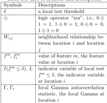
3.1 List of symbols and descriptions . . . 41

3.2 Simplified cost model with different numbers of distinct feature values (Nd) 57 3.3 Classification performance of LTDT, FTSDT-fixed, FTSDT-adaptive . . 59

3.4 Kˆ statistics of confusion matrices . . . 59

3.5 Significance test on difference of confusion matrices . . . 60

3.6 Description of datasets . . . 60

4.1 Comparison of classification performance on Chanhassen Data . . . 83

4.2 Comparison of classification performance on Swan Lake Data . . . 84

4.3 Comparison of classification performance on Big Stone Data . . . 84

(12)

List of Figures

1.1 The process of spatial big data analytics. . . 2

3.1 Real world problem example . . . 36

3.2 Related work classification . . . 37

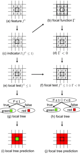
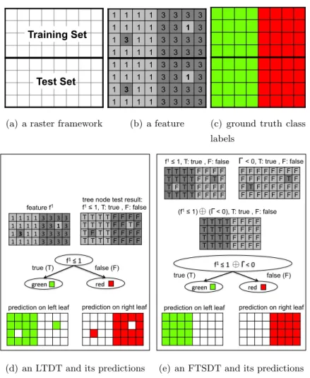
3.3 Example of a spatial raster framework and a neighborhood relationship 39 3.4 Comparison of a local test v.s. a focal test, a local-test-based decision tree v.s. a focal-test-based spatial decision tree. (“T” is “true”, “F” is “false”) . . . 40

3.5 An illustrative problem example (best viewed in color). . . 43

3.6 Comparison of focal tests with fixed and adaptive neighborhoods,s= 2 (i.e., 5 by 5 window). . . 49

3.7 Computational bottleneck analysis in training algorithms . . . 51

3.8 Illustrative example of redundant focal Γ computation. . . 52

3.9 Experiment Design . . . 59

3.10 Case study dataset and prediction results of LTDT and FTSDT. . . 62

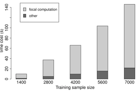
3.11 Computational performance comparison between basic and refined algo-rithms . . . 64

3.12 Computational performance comparison on different image sizes . . . 66

4.1 Real world example of geographical classification with class ambiguity: class ambiguity exists in two white circles of (a) (best viewed in color) . 69 4.2 Related work summary . . . 71

4.3 Illustrative example of problem inputs and outputs . . . 72

4.4 Interpretation of class ambiguity for binary class . . . 73

4.5 Illustrative examples of related work approaches (best viewed in color) . 75 4.6 Illustrative example of patch generation . . . 77

(13)

footprint 1, patches in bold solid line belong to footprint 2 (best viewed

in color) . . . 80

4.8 Experiment Setup . . . 82

4.9 Effect of the number of training samples . . . 85

4.10 Effect of the base classifier type . . . 86

4.11 Sensitivity to number of patches in preprocessing . . . 87

4.12 Comparison with related work adding spatial coordinate features in de-cision tree, random forests, and mixture of experts (black and blue are errors, best viewed in color) . . . 88

4.13 Real world case study in Chanhassen (best viewed in color) . . . 89

4.14 Real world case study in Swan Lake (best viewed in color) . . . 92

4.15 Real world case study in Big Stone (best viewed in color) . . . 93

(14)

Chapter 1

Introduction

1.1 Spatial Big Data Analytics

Spatial big data (SBD) is geo-referenced data whose volume, velocity, and variety ex-ceed the capability of current common spatial computing platforms. Examples of SBD include GPS trajectories (1013_{records per year), earth observation imagery (10}15_bytes per year by NASA only), and check-in location history (106 _{per day). Spatial big data} analytic is the process of discovering interesting, previously unknown, but potentially useful patterns from SBD. Figure 1.1 shows the entire knowledge discovery process. The core component is spatial big data analytic algorithms, which take input spatial big data and produce desired output pattern families, including spatial or spatiotemporal outliers, associations and tele-connections, predictive models, partitions and summa-rization, hotspots, as well as change patterns. For example, spatial prediction can be used to classify earth observation images into different land cover types. Spatial colo-cation patterns can identify crime event types that frequently occur together. These algorithms have statistical foundations and integrate scalable computational techniques and platforms. The type of input data and the choice of output patterns often determine which kind of algorithms are appropriate to use.

(15)

Input Spatial Big Data

Preprocessing, Exploratory

Space-Time Analysis _{Analytic Algorithm}Spatial Big Data Patterns Output Post-processing

Interpretation by Domain Experts

Spatial Statistics Computational platforms and techniques

Figure 1.1: The process of spatial big data analytics.

1.2 Societal Applications

Spatial big data analytics are crucial to organizations which make decisions based on large spatial and spatiotemporal datasets, including NASA, the National Geospatial-Intelligence Agency, the National Cancer Institute, the US Department of Transporta-tion, and the National Institute of Justice. These organizations are spread across many application domains. In ecology and environmental management, researchers need tools to classify remote sensing images to map forest coverage. In public safety, crime analysts are interested in discovering hotspot patterns from crime event maps so as to effectively allocate police resources. In transportation, researchers analyze historical taxi GPS tra-jectories to recommend fast routes from places to places. Epidemiologists use spatial big data techniques to detect disease outbreak. There are also other application domains such as earth science, climatology, precision agriculture, and Internet of Things.

The interdisciplinary nature of spatial big data analytics means that techniques must be developed with awareness of the underlying physics or theories in their application domains [41]. For example, climate science studies find that observable predictors for climate phenomena discovered by data driven techniques can be misleading if they do not take into account climate models, locations, and seasons [42]. In this case, statis-tical significance testing is cristatis-tically important in order to further validate or discard relationship patterns mined from data.

1.3 Challenges

Spatial big data analytics pose unique statistical and computational challenges. In addition to its huge volume, SBD has the following unique characteristics that challenge

(16)

current big data analytic techniques.

1.3.1 Spatial Autocorrelation

According to Tobler’s first law of geography, “Everything is related to everything else, but near things are more related than distant things.” For example, people with sim-ilar characteristics, occupation and background tend to cluster together in the same neighborhood. In spatial statistics, such spatial dependence is called the spatial au-tocorrelation effect. Ignoring auau-tocorrelation and assuming an identical and indepen-dent distribution (i.i.d.) when analyzing data with spatial characteristics may produce hypotheses or models that are inaccurate or inconsistent with the data set [2] (e.g., salt-and-pepper noise in remote sensing image classification). Similarly, due to the fact that spatial big data is embedded in continuous space, many classical data mining tech-niques assuming discrete data (e.g., transactions in association rule mining) may not be effective (e.g., breaking neighboring locations into different transactions).

1.3.2 Spatial Anisotropy

Another challenge is that the degree of spatial dependency also varies across different directions (also called spatial anisotropy) due to irregular geographical terrains, topolog-ical relationships, etc. For example, biogeographtopolog-ical patterns on river networks are often constrained by the network topological structure and flow directions. Many current spa-tial statistics assume isotropy and use spaspa-tial neighborhoods with regular shapes (e.g., square window) to model spatial dependency. This may result in inaccurate models and predictions.

1.3.3 Multi-scale Effect

Modifiable area unit problem (MAUP) or multi-scale effect is another challenge since results of spatial analysis depends on the choice of an appropriate spatial scale (e.g., local, regional, global). For example, spatial autocorrelation values at local level may be significantly different from values at global level, especially when spatial outliers exist. As another instance of example, patterns of spatial interactions between two types of events may be significant in one region of the study area, but insignificant in other areas.

(17)

1.3.4 Spatial Heterogeneity

The last challenge is the spatial heterogeneity, i.e., spatial data samples do not follow an identical distribution across the entire space. One type of spatial heterogeneity is that samples with the same explanatory features may belong to different class labels in different zones. For example, upland forest looks very similar to wetland forest in spectral values on remote sensing images, but they are from different land cover classes due to different geographical terrains. Another types of spatial heterogeneity is different trends between explanatory variables and response variable in different locations. For instance, in economic studies, it may be possible that old houses are with high price in rural areas, but with low price in urban areas. Though house age is not an effective coefficient for house price when the entire study area is considered, it is an effective coefficient in each local areas (rural or urban).

One way to deal with implicit spatial relationships is to materialize the relation-ships into traditional data input columns and then apply classical big data analytic techniques. However, the materialization can result in loss of information [2]. Another issue is the existence of a semantic gap between traditional big data algorithms and spatial and spatiotemporal data. For example, Ring-shaped hotspot pattern is very important in environmental criminology but is hard to characterize in the matrix space as in traditional data mining. Finally, many traditional data mining methods are not spatial or spatiotemporal statistical aware and thus prone to produce spurious spatial patterns. A more preferable way to capture implicit spatial and temporal relationships is to develop statistics and techniques to incorporate spatial and temporal information into the data analytic process.

1.4 Contributions

In this thesis, we overview current spatial data analytic techniques, and introduce two novel spatial big data classification approaches, i.e., spatial decision tree, and spatial ensemble learning, which address some of the above challenges.

(18)

• Chapter 2 surveys current techniques in spatial and spatiotemporal data min-ing. Spatial and spatiotemporal (SST) data mining studies the process of discov-ering interesting, previously unknown, but potentially useful patterns from large SST databases. It has broad application domains including ecology, environmen-tal management, public safety, etc. The complexity of input data and intrinsic spatial and spatiotemporal relationships limits the usefulness of conventional data mining methods. We review recent computational techniques in SST data mining. Compared with other surveys, this chapter emphasizes the statistical foundation and proposes a taxonomy of major pattern families to categorize recent research.

• Chapter 3 discusses a novel spatial classification technique called spatial deci-sion tree to address the challenge of spatial autocorrelation and anisotropy. Given learning samples from a raster dataset, spatial decision tree learning aims to find a decision tree classifier that minimizes classification errors as well as salt-and-pepper noise. The problem has important societal applications such as land cover classification for natural resource management. However, the problem is challeng-ing due to the fact that learnchalleng-ing samples show spatial autocorrelation in class labels, instead of being independently identically distributed. Related work relies on local tests (i.e., testing feature information of a location) and cannot adequately model the spatial autocorrelation effect, resulting in salt-and-pepper noise. In con-trast, we recently proposed a focal-test-based spatial decision tree (FTSDT), in which the tree traversal direction of a sample is based on both local and focal (neighborhood) information. Preliminary results showed that FTSDT reduces classification errors and salt-and-pepper noise. We also extend our recent work by introducing a new focal test approach with anisotropic spatial neighborhoods that avoids over-smoothing in wedge-shaped areas. We also conduct computational refinement on the FTSDT training algorithm by reusing focal values across can-didate thresholds. Theoretical analysis shows that the refined training algorithm is correct and more scalable. Experiment results on real world datasets show that new FTSDT with adaptive neighborhoods improves classification accuracy, and that our computational refinement significantly reduces training time.

(19)

• Chapter 4discusses a novel ensemble learning framework called spatial ensemble to address the challenge of spatial heterogeneity. Given geographical data with class ambiguity, i.e., samples with similar features belonging to different classes in different zones, the spatial ensemble learning (SEL) problem aims to find a decomposition of the geographical area into disjoint zones minimizing class am-biguity and to learn a local classifier in each zone. Class amam-biguity is a common issue in many geographical classification applications. For example, in remote sensing image classification, pixels with the same spectral signatures may corre-spond to different land cover classes in different locations due to heterogeneous geographical terrains. A global classifier may mistakenly classify those ambigu-ous pixels into one land cover class. However, SEL problem is challenging due to class ambiguity issue, unknown and arbitrary shapes of zonal footprints, and high computational cost due to the potential exponential number of candidate zonal partitions. Related work in ensemble learning either assumes an identical and independent distribution of input data (e.g., bagging, boosting) or decomposes multi-modular input data in the feature vector space (e.g., mixture of experts), and thus cannot effectively decompose the input data in geographical space to reduce class ambiguity. In contrast, we propose a spatial ensemble learning frame-work that explicitly partition input data in geographical space: first, the input data is preprocessed into homogeneous “patches” via constrained hierarchical spa-tial clustering; second, patches are grouped into several footprints via greedy seed growing and spatial adjustments. Experimental evaluation on three real world re-mote sensing datasets show that the proposed approach outperforms related work in classification accuracy.

(20)

Chapter 2

Spatial and Spatiotemporal Data

Mining Overview

This chapter overviews the state of the art spatial and spatial temporal data mining techniques. Current overview tutorials and surveys in spatial and spatiotemporal data mining can be categorized into two groups: early papers in the 1990s without a focus on spatial and spatiotemopral statistical foundations, and recent papers with a focus on statistical foundation. Two early survey papers [43, 44] review spatial data mining from a database approach. Recent papers include brief tutorials on current spatial [45] and spatiotemporal data mining [46] techniques. There are also other relevant book chapters [47, 48, 2], as well as survey papers on specific spatial or spatiotemporal data mining tasks such as spatiotemporal clustering [49], spatial outlier detection [50], and spatial and spatiotemporal change footprint detection [51].

This chapter makes the following contributions: (1) we provide a categorization of input spatial and spatiotemporal data types; (2) we provide a summary of spatial and spatiotemporal statistical foundations categorized by different data types; (3) we create a taxonomy of six major output pattern families, including spatial and spatiotemporal outliers, associations and tele-connections, predictive models, partitioning (clustering) and summarization, hotspots and changes. Within each pattern family, common compu-tational approaches are categorized by the input data types; (4) we analyze the research trends and future research needs.

(21)

Organization of the chapter: This chapter starts with a summary of input spa-tial and spatiotemporal data (Section 2.1) and an overview of statistical foundation (Section 2.2). It then describes in detail six main output pattern families including spa-tial and spatiotemporal outliers, associations and tele-connections, predictive models, partitioning (clustering) and summarization, hotspots, and changes (Section 2.3). An examination of research trend and future research needs is in Section 2.4. Section 2.5 summarizes the chapter.

2.1 Input: Spatial and Spatiotemporal Data

2.1.1 Types of Spatial and Spatiotemporal Data

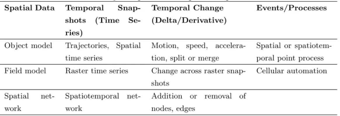
The data inputs of spatial and spatiotemporal data mining tasks are more complex than the inputs of classical data mining tasks because they include discrete representations of continuous space and time. Table 2.1 gives a taxonomy of different spatial and spatiotemporal data types (or models). Spatial data can be categorized into three models, i.e., the object model, the field model, and the spatial network model [40, 52]. Spatiotemporal data, based on how temporal information is additionally modeled, can be categorized into three types, i.e., temporal snapshot model, temporal change model, and event or process model [53, 54, 55]. In the temporal snapshot model, spatial layers of the same theme are time-stamped. For instance, if the spatial layers are points or multi-points, their temporal snapshots are trajectories of points or spatial time series (i.e., variables observed at different times on fixed locations). Similarly, snapshots can represent trajectories of lines and polygons, raster time series, and spatiotemporal networks such as time expanded graphs (TEGs) and time aggregate graphs (TEGs) [56, 57]. The temporal change model represents spatiotemporal data with a spatial layer at a given start time together with incremental changes occurring afterward. For instance, it can represent motion (e.g., Brownian motion, random walk [5]) as well as speed and acceleration on spatial points, as well as rotation and deformation on lines and polygons. Event and process models represent temporal information in terms ofevents

(22)

whose properties are possessed timelessly and therefore are not subject to change over time, whereas processes are entities that are subject to change over time (e.g., a process may be said to be accelerating or slowing down) [58].

Table 2.1: Taxonomy of Spatial and Spatiotemporal Data Models.

Spatial Data Temporal Snap-shots (Time Se-ries)

Temporal Change (Delta/Derivative)

Events/Processes

Object model Trajectories, Spatial time series

Motion, speed, accelera-tion, split or merge

Spatial or spatiotem-poral point process Field model Raster time series Change across raster

snap-shots Cellular automation Spatial net-work Spatiotemporal net-work Addition or removal of nodes, edges

2.1.2 Data Attributes and Relationships

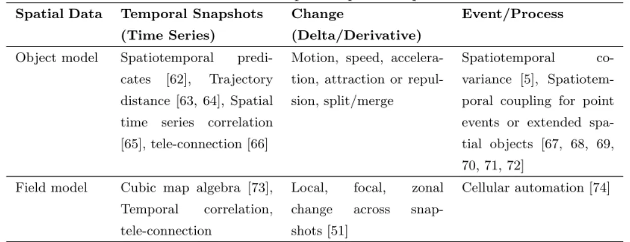
There are three distinct types of data attributes for spatiotemporal data, including non-spatiotemporal attributes, spatial attributes, and temporal attributes. Non spa-tiotemporal attributes are used to characterize non-contextual features of objects, such as name, population, and unemployment rate for a city. They are the same as the attributes used in the data inputs of classical data mining [59]. Spatial attributes are used to define the spatial location (e.g., longitude and latitude), spatial extent (e.g., area, perimeter) [60, 61], shape, as well as elevation defined in a spatial reference frame. Temporal attributes include the timestamp of a spatial object, a raster layer, or a spa-tial network snapshot, as well as the duration of a process. Relationships on non-spaspa-tial attributes are often explicit, including arithmetic, ordering, and subclass, etc. Relation-ships on spatial attributes, in contrast, are often implicit, including those in topological space (e.g., meet, within, overlap), set space (e.g., union, intersection), metric space (e.g., distance) and directions. Relationships on spatiotemporal attributes are more sophisticated, as summarized in Table 2.2.

(23)

Table 2.2: Relationships on Spatiotemporal Data.

Spatial Data Temporal Snapshots (Time Series)

Change

(Delta/Derivative)

Event/Process

Object model Spatiotemporal predi-cates [62], Trajectory distance [63, 64], Spatial time series correlation [65], tele-connection [66]

Motion, speed, accelera-tion, attraction or repul-sion, split/merge

Spatiotemporal co-variance [5], Spatiotem-poral coupling for point events or extended spa-tial objects [67, 68, 69, 70, 71, 72]

Field model Cubic map algebra [73], Temporal correlation, tele-connection

Local, focal, zonal change across snap-shots [51]

Cellular automation [74]

One way to deal with implicit spatiotemporal relationships is to materialize the re-lationships into traditional data input columns and then apply classical data mining techniques [75, 76, 77, 78, 79]. However, the materialization can result in loss of in-formation [2]. The spatial and temporal vagueness which naturally exists in data and relationships usually creates further modeling and processing difficulty in spatial and spatiotemporal data mining. A more preferable way to capture implicit spatial and spa-tiotemporal relationships is to develop statistics and techniques to incorporate spatial and temporal information into the data mining process. These statistics and techniques are the main focus the survey.

2.2 Statistical Foundations

2.2.1 Spatial Statistics for Different Types of Spatial Data

Spatial statistics [3, 4, 5, 6] is a branch of statistics concerned with the analysis and modeling of spatial data. The main difference between spatial statistics and classical statistics is that spatial data often fails to meet the assumption of an identical and independent distribution (i.i.d.). As summarized in Table 2.3, spatial statistics can be categorized according to their underlying spatial data type: Geostatistics for point

(24)

referenced data, lattice statistics for areal data, and spatial point process for spatial point patterns.

Geostatistics: Geostatistics [6] deal with the analysis of the properties of point

reference data, including spatial continuity (i.e., dependence across locations), weak stationarity (i.e., first and second moments do not vary with respect to locations) and isotropy (i.e., uniformity in all directions). For example, under the assumption of weak stationarity (or more specifically intrinsic stationarity), variance of the difference of non-spatial attribute values at two point locations is a function of point location difference regardless of specific point locations. This function is called a variogram [29]. If the variogram only depends on distance between two locations (not varying with respect to directions), it is further called isotropic. Under the assumptions of these properties, Geostatistics also provides a set of statistical tools such as Kriging [29], which can be used to interpolate non-spatial attribute values at unsampled locations. Finally, real world spatial data may not always satisfy the stationarity assumption. For example, different jurisdictions tend to produce different laws (e.g., speed limit differences between Minnesota and Wisconsin). This effect is called spatial heterogeneity or non-stationarity. Special models (e.g., geographically weighted regression, or GWR [37]) can be further used to model the varying co-efficients at different locations.

Lattice statistics: Lattice statistics studies statistics for spatial data in the field (or

areal) model. Here a lattice refers to a countable collection of regular or irregular cells in a spatial framework. The range of spatial dependency among cells is reflected by a neighborhood relationship, which can be represented by a contiguity matrix called a W-matrix. A spatial neighborhood relationship can be defined based on spatial ad-jacency (e.g., rook or queen neighborhoods) or Euclidean distance, or in more general models, cliques and hypergraphs [9]. Based on a W-matrix, spatial autocorrelation statistics can be defined to measure the correlation of a non-spatial attribute across neighboring locations. Common spatial autocorrelation statistics include Moran’s I, Getis-Ord Gi∗, Geary’s C, Gamma index Γ [7], etc., as well as their local versions called local indicators of spatial association (LISA) [10]. Several spatial statistical mod-els, including the spatial autoregressive model (SAR), conditional autoregressive model (CAR), Markov random fields (MRF), as well as other Bayesian hierarchical models [3], can be used to model lattice data. Another important issue is the modifiable areal unit

(25)

problem (MAUP) (also called the multi-scale effect) [11], an effect in spatial analysis that results for the same analysis method will change on different aggregation scales. For example, analysis using data aggregated by states will differ from analysis using data at individual family level.

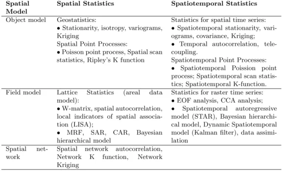
Table 2.3: Taxonomy of Spatial and Spatiotemporal Statistics.

Spatial Model

Spatial Statistics Spatiotemporal Statistics

Object model Geostatistics:

•Stationarity, isotropy, variograms, Kriging

Spatial Point Processes:

•Poisson point process, Spatial scan statistics, Ripley’s K function

Statistics for spatial time series: •Spatiotemporal stationarity, vari-ograms, covariance, Kriging; • Temporal autocorrelation, tele-coupling.

Spatiotemporal Point Processes: • Spatiotemporal Poission point process; Spatiotemporal scan statis-tics; Spatiotemporal K-function. Field model Lattice Statistics (areal data

model):

•W-matrix, spatial autocorrelation, local indicators of spatial associa-tion (LISA);

• MRF, SAR, CAR, Bayesian hierarchical model

Statistics for raster time series: •EOF analysis, CCA analysis; • Spatiotemporal autoregressive model (STAR), Bayesian hierarchi-cal model, Dynamic Spatiotemporal model (Kalman filter), data assimi-lation

Spatial net-work

Spatial network autocorrelation, Network K function, Network Kriging

Spatial point processes: A spatial point process is a model for the spatial distribution

of the points in a point pattern. It differs from point reference data in that the random variables are locations. Examples include positions of trees in a forest and locations of bird habitats in a wetland. One basic type of point process is a homogeneous spa-tial Poisson point process (also called complete spaspa-tial randomness, or CSR) [5], where point locations are mutually independent with the same intensity over space. However, real world spatial point processes often show either spatial aggregation (clustering) or spatial inhibition instead of complete spatial independence as in CSR. Spatial statistics such as Ripley’s K function [12, 13], i.e., the average number of points within a certain distance of a given point normalized by the average intensity, can be used to test spatial aggregation of a point pattern against CSR. Moreover, real world spatial point processes

(26)

such as crime events often contain hotspot areas instead of following homogeneous in-tensity across space. A spatial scan statistic [14] can be used to detect these hotspot patterns. It tests if the intensity of points inside a scanning window is significantly higher (or lower) than outside. Though both the K-function and spatial scan statistics have the same null hypothesis of CSR, their alternative hypotheses are quite different: the K-function tests if points exhibit spatial aggregation or inhibition instead of inde-pendence, while spatial scan statistics assume that points are independent and test if a local hotspot with much higher intensity than outside exists. Finally, there are other spatial point processes such as the Cox process, in which the intensity function itself is a random function over space, as well as a cluster process, which extends a basic point process with a small cluster centered on each original point [5]. For extended spatial objects such as lines and polygons, spatial point processes can be generalized to line processes and flat processes in stochastic geometry [15].

Spatial network statistics: Most spatial statistics research focuses on the Euclidean

space. Spatial statistics on the network space are much less studied. Spatial network space, e.g., river networks and street networks, is important in applications of environ-mental science and public safety analysis. However, it poses unique challenges including directionality and anisotropy of spatial dependency, connectivity, as well as high com-putational cost. Statistical properties of random fields on a network are summarized in [16]. Recently, several spatial statistics, such as spatial autocorrelation, K-function, and Kriging, have been generalized to spatial networks [17, 18, 19]. Little research has been done on spatiotemporal statistics on the network space.

2.2.2 Spatiotemporal Statistics

Spatiotemporal statistics [80, 5] combine spatial statistics with temporal statistics (time series analysis [81], dynamic models [80]). Table 2.3 summarizes common statistics for different spatiotemporal data types, including spatial time series, spatiotemporal point process, and time series of lattice (areal) data.

Spatial time series: Spatial statistics for point reference data have been generalized

for spatiotemporal data [82]. Examples include spatiotemporal stationarity, spatiotem-poral covariance, spatiotemspatiotem-poral variograms, and spatiotemspatiotem-poral Kriging [80, 5]. There is also temporal autocorrelation and tele-coupling (high correlation across spatial time

(27)

series at a long distance). Methods to model spatiotemporal process include physics inspired models (e.g., stochastically differential equations) [5] and hierarchical dynamic spatiotemporal models (e.g., Kalman filtering) for data assimilation [5].

Spatiotemporal point process: A spatiotemporal point process generalizes the spatial

point process by incorporating the factor of time. As with spatial point processes, there are spatiotemporal Poisson process, Cox process, and cluster process. There are also corresponding statistical tests including a spatiotemporal K function and spatiotemporal scan statistics [5].

Time series of lattice (areal) data: Similar to lattice statistics, there are spatial and

temporal autocorrelation, SpatioTemporal Autoregressive Regression (STAR) model [83], and Bayesian hierarchical models [3]. Other spatiotemporal statistics include empiri-cal orthogonal function (EOF) analysis (principle component analysis in geophysics), canonical-correlation analysis (CCA), and dynamic spatiotemporal models (Kalman fil-ter) for data assimilation [80].

2.3 Output Pattern Families

2.3.1 Spatial and Spatiotemporal Outlier Detection

This section reviews techniques for spatial and spatiotemporal outlier detection. The section begins with a definition of spatial or spatiotemporal outliers by comparison with global outliers. Spatial and spatiotemporal outlier detection techniques are summarized according to their input data types.

Problem definition: To understand the meaning of spatial and spatiotemporal

out-liers, it is useful first to consider global outliers. Global outliers [84, 85] have been informally defined as observations in a data set which appear to be inconsistent with the remainder of that set of data, or which deviate so much from other observations as to arouse suspicions that they were generated by a different mechanism. In contrast, a spa-tial outlier [86] is a spaspa-tially referenced object whose non-spaspa-tial attribute values differ significantly from those of other spatially referenced objects in its spatial neighborhood. Informally, a spatial outlier is a local instability or discontinuity. For example, a new house in an old neighborhood of a growing metropolitan area is a spatial outlier based on the non-spatial attribute house age. Similarly, a spatiotemporal outlier generalizes

(28)

spatial outliers with a spatiotemporal neighborhood instead of a spatial neighborhood.

Statistical foundation: The spatial statistics for spatial outlier detection are also

applicable to spatiotemporal outliers as long as spatiotemporal neighborhoods are well-defined. The literature provides two kinds of bi-partite multidimensional tests: graphical tests, including variogram clouds [87] and Moran scatterplots [10, 6], and quantitative tests, including scatterplot [88] and neighborhood spatial statistics [86].

Spatial outlier detection

Thevisualization approach plots spatial locations on a graph to identify spatial outliers.

The common methods are variogram clouds and Moran scatterplot as introduced earlier.

The neighborhood approach defines a spatial neighborhood, and a spatial statistic

is computed as the difference between the non-spatial attribute of the current location and that of the neighborhood aggregate [86]. Spatial neighborhoods can be identified by distance on spatial attributes (e.g., K nearest neighbors), or by graph connectivity (e.g., locations on road networks). This work has been extended in a number of ways to allow for multiple non-spatial attributes [89], average and median attribute value [90], weighted spatial outliers [91], categorical spatial outlier [92], local spatial outliers [93], and fast detection algorithms [94].

Spatiotemporal Outlier Detection

The intuition behind spatiotemporal outlier detection is that they reflect “discontinuity” on non-spatiotemporal attributes within a spatiotemporal neighborhood. Approaches can be summarized according to the input data types.

Outliers in spatial time series: For spatial time series (on point reference data,

raster data, as well as graph data), basic spatial outlier detection methods, such as visualization based approaches and neighborhood based approaches, can be generalized with a definition of spatiotemporal neighborhoods.

Flow Anomalies: Given a set of observations across multiple spatial locations on a

spatial network flow, flow anomaly discovery aims to identify dominant time intervals where the fraction of time instants of significantly mis-matched sensor readings exceeds the given percentage-threshold. Flow anomaly discovery can be considered as detecting

(29)

discontinuities orinconsistencies of a non-spatiotemporal attribute within a neighbor-hood defined by the flow between nodes, and such discontinuities are persistent over a period of time. A time-scalable technique called SWEET (Smart Window Enumer-ation and EvaluEnumer-ation of persistent-Thresholds) was proposed [95] that utilizes several algebraic properties in the flow anomaly problem to discover these patterns efficiently.

2.3.2 Spatial and Spatiotemporal Associations, Tele-connections

This section reviews techniques for identifying spatial and spatiotemporal association as well as tele-connections. The section starts with the basic spatial association (or location) pattern, and moves on to spatiotemporal association (i.e., spatiotemporal co-occurrence, cascade, and sequential patterns) as well as spatiotemporal tele-connection.

Pattern definition: Spatial association, also known as spatial co-location patterns [96],

represent subsets of spatial event types whose instances are often located in close geographic proximity. Real-world examples include symbiotic species, e.g., the Nile Crocodile and Egyptian Plover in ecology. Similarly, spatiotemporal association pat-terns represent spatiotemporal object types whose instances often occur in close geo-graphic and temporal proximity. Spatiotemporal coupling patterns can be categorized according to whether there exists temporal ordering of object types: spatiotemporal (mixed drove) co-occurrences [97] are used for unordered patterns, spatiotemporal cas-cades [69] for partially ordered patterns, and spatiotemporal sequential patterns [71] for totally ordered patterns. Spatiotemporal tele-connection [65] represents patterns of significantly positive or negative temporal correlation between a pair of spatial time series.

Challenges: Mining patterns of spatial and spatiotemporal association is challenging

due to the following reasons: first, there is no explicit transaction in continuous space and time; second, there is potential for over-counting; third, the number of candidate patterns is exponential, and a trade-off between statistical rigor of output patterns and computational efficiency has to be made.

Statistical foundation: The underlying statistic for spatiotemporal coupling patterns

is the cross K function, which generalizes the basic Ripley’s K function (introduced in Section 2.2) for multiple event types.

(30)

approaches for discovering spatial and spatiotemporal couplings by different input data types.

Spatial colocation: Mining colocation patterns can be done via statistical approaches

including cross-K function with Monte Carlo simulation [6], mean nearest-neighbor dis-tance, and spatial regression model [98], but these methods are often computation-ally very expensive due to the exponential number of candidate patterns. In contrast, data mining approaches aim to identify colocation patterns like association rule min-ing. Within this category, there are transaction based approaches and distance based approaches. A transaction based approach defines transactions over space (e.g., around instances of a reference feature) and then uses an Apriori-like algorithm [99]. A distance based approach defines a distance-based pattern called k-neighboring class sets [100] or using an event centric model [96] based on a definition of participation index, which is an upper bound of cross-K function statistic and has an anti-monotone property. Recently, approaches have been proposed to identify colocations for extended spatial objects [101] or rare events [102], regional colocation patterns [103, 104] (i.e., pattern is significant only in a sub-region), statistically significant colocation [105], as well as design fast algorithms [106].

Spatiotemporal events associations represent subsets of two or more event-types

whose instances are often located in close spatial and temporal proximity. Spatiotem-proal event associations can be categorized into spatiotemporal co-occurrences,

spa-tiotemporal cascades, and spatiotemporal sequential patterns for temporally unordered

events, partially ordered events, and totally ordered events respectively. To discover spa-tiotemporal co-occurrences, a monotonic composite interest measure and novel mining algorithms are presented in [97]. A filter-and-refine approach has also been proposed to identify spatiotemporal co-occurrences on extended spatial objects [68]. A spatiotem-poral sequential pattern represents a “chain reaction” from different event types. A measure of sequence index, which can be interpreted by K-function statistic, was pro-posed in [71], together with computationally efficient algorithms. For spatiotemporal cascade patterns, a statistically meaningful metric was proposed to quantify interest-ingness and pruning strategies were proposed to improve computational efficiency [69].

Spatiotemporal association from moving objects trajectories: Mining spatiotemporal

(31)

data due to the existence of temporal duration, different moving directions, and impre-cise locations. There are a variety of ways to define spatiotemporal association patterns from moving object trajectories. One way is to generalize the definition from spatiotem-poral event data. For example, a pattern called spatiotemspatiotem-poral colocation episodes is defined to identify frequent sequences of colocation patterns that share a common event (object) type [107]. As another example, a spatiotemporal sequential pattern is defined based on decomposition of trajectories into line segments and identification of frequent region sequences around the segments [108]. Another way is to define spatiotemporal association as group of objects that frequently move together, either focusing on the footprints of subpaths (region sequences) that are commonly traversed [109] or subsets of objects that frequently move together (also called travel companion) [110].

Spatial time series oscillation and tele-connection: Given a collection of spatial time

series at different locations, tele-connection discovery aims to identify pairs of spatial time series whose correlation is above a given threshold. Tele-connection patterns are important in understanding oscillations in climate science. Computational challenges arise from the large number of candidate pairs and the length of time series. An efficient index structure, called a cone-tree, as well as a filter and refine approach [65] have been proposed which utilize spatial autocorrelation of nearby spatial time series to filter out redundant pair-wise correlation computation. Another challenge is the existence of spu-rious ‘high correlation’ patterns that happen by chance. Recently, statistical significant tests have been proposed to identify statistically significant tele-connection patterns called dipoles from climate data [66]. The approach uses a “wild bootstrap” to capture the spatio-temporal dependencies, and takes account of the spatial autocorrelation, the seasonality and the trend in the time series over a period of time.

2.3.3 Spatial and Spatiotemporal Prediction

Problem definition: Given training samples with features and a target variable as well

as a spatial neighborhood relationship among samples, the problem of spatial prediction

aims to learn a model that can predict the target variable based on features. What distinguishes spatial prediction from traditional prediction problem in data mining is that data items are embedded in space, and often violate the common assumption of an identical and independent distribution (i.i.d.). Spatial prediction problems can

(32)

be further categorized into spatial classification for nominal (i.e., categorical) target variables and spatial regression for numeric target variables.

Challenges: The unique challenges of spatial and spatiotemporal prediction come

from the special characteristics of spatial and spatiotemporal data, which include spa-tial and temporal autocorrelation, spaspa-tial heterogeneity and temporal non-stationarity, as well as the multi-scale effect. These unique characteristics violate the common as-sumption in many traditional prediction techniques that samples follow an identical and independent distribution (i.i.d.). Simply applying traditional prediction techniques without incorporating these unique characteristics may produce hypotheses or models that are inaccurate or inconsistent with the data set.

Statistical foundations: Spatial and spatiotemporal prediction techniques are

de-veloped based on spatial and spatiotemporal statistics, including spatial and temporal autocorrelation, spatial heterogeneity, temporal non-stationarity, and multiple areal unit problems (MAUP) (see Section 2.2).

Computational approaches: The following subsections summarize common spatial

and spatiotemporal prediction approaches for different data types. We further catego-rize these approaches according to the challenges that they address, including spatial and spatiotemporal autocorrelation, spatial heterogeneity, spatial multi-scale effect, and temporal non-stationarity, and introduce each category separately below.

Spatial Autocorrelation or Dependency

According to Tobler’s first law of geography [20], “everything is related to everything else, but near things are more related than distant things.” The spatial autocorrelation effect tells us that spatial samples are not statistically independent, and nearby samples tend to resemble each other. There are different ways to incorporate the effect of spatial autocorrelation or dependency into predictive models, including spatial feature creation, explicit model structure modification, and spatial regularization in objective functions.

Spatial feature creation: The main idea is to create new features that incorporate

spatial contextual (neighborhood) information. Spatial features can be generated di-rectly from spatial aggregation [21], indidi-rectly from multi-relationship (or spatial as-sociation) rules between spatial entities [22, 23, 24], or from spatial transformation of raw features [25]. After spatial features are generated, they can be fed into a general

(33)

prediction model. One advantage of this approach is that it could utilize many existing predictive models without significant modification. However, spatial feature creation in preprocessing phase is often application specific and time consuming.

Spatial interpolation: Given observations of a variable at a set of locations (point

ref-erence data), spatial interpolation aims to measure the variable value at an unsampled location [26]. These techniques are broadly classified into three categories: geostatis-tical, non-geosatistical and some combined approaches. Among the non-geostatistical approaches, the nearest neighbors, inverse distance weighting, etc. are the mostly used techniques in literature. Kriging is the most widely used geo-statistical interpolation technique, which represents a family of generalized least-squares regression based in-terpolation techniques [27]. Kriging can be broadly classified into two categories: uni-variate (only variable to be predicted) and multiuni-variate (there are some covariates, also called explanatory variables). Unlike the non-geostatistical or traditional interpolation techniques, this estimator considers both the distance, as well as the degree of varia-tion between the sampled and unsampled locavaria-tions for the random variable estimavaria-tion. Among the univariate kriging methods, thesimple kriging,ordinary kriging and in mul-tivariate scenario, the ordinary co-kriging, universal kriging and kriging with external

drift are the most popular and widely used technique in the study of spatial

interpola-tion [26, 28]. However, the kriging suffers from some acute shortcomings of assuming the isotopic nature of the random variables.

Markov Random Field (MRF): MRF [29] is a widely used model in image

classifi-cation problems. It assumes that the class label of one pixel only depends on the class labels of its predefined neighbors (also called Markov property). In spatial classification problem, MRF is often integrated with other non-spatial classifiers to incorporate the spatial autocorrelation effect. For example, MRF has been integrated with maximum likelihood classifiers (MLC) to create Markov Random Field (MRF)-based Bayesian classifiers [30], in order to avoid salt-and-pepper noise in prediction [31]. Another ex-ample is the model of Support Vector Random Fields [32].

Spatial Autoregressive Model (SAR):In the spatial autoregression model, the spatial

dependencies of the error term, or, the dependent variable, are directly modeled in the regression equation [33]. If the dependent values yi are related to each other, then the

(34)

regression equation can be modified as y =ρW y+Xβ+, where W is the neighbor-hood relationship contiguity matrix and ρ is a parameter that reflects the strength of the spatial dependencies between the elements of the dependent variable. For spatial classification problems, logistic transformation can be applied to SAR model for binary classes.

Conditional autoregressive model (CAR):In the conditional autoregressive model [29],

the spatial autocorrelation effect is explicitly modeled by the conditional probability of the observation of a location given observations of neighbors. CAR is essentially a Markov random field. It is often used as a spatial term in Bayesian hierarchical models.

Spatial accuracy objective function: In traditional classification problems, the

ob-jective function (or loss function) often measures the zero-one loss on each sample, no matter how far the predicted class is from the location of the actuals. For example, in bird nest location prediction problem on a rasterized spatial field, a cell’s predicted class (e.g., bird nest) is either correct or incorrect. However, if a cell mistakenly predicted as the bird nest class is very close to an actual bird nest cell, the prediction accuracy should not be considered as zero. Thus, spatial accuracy [34, 35] has been proposed to measure not only how accurate each cell is predicted itself but also how far it is from an actual class locations. A case study has shown that learning models based on proposed objective function produce better accuracy in bird nest location prediction problem. Spatial objective function has also been proposed in active learning [36], in which the cost of additional label not only consider accuracy but also travel cost between locations to be labeled.

Spatial Heterogeneity

Spatial heterogeneity describes the fact that samples often do not follow an identical distribution in the entire space due to varying geographic features. Thus, a global model for the entire space fails to capture the varying relationships between features and the target variable in different sub-region. The problem is essentially the multi-task learning problem, but a key challenge is how to identify different multi-tasks (or regional or local models). Several approaches have been proposed to learn local or regional models. Some approaches first partition the space into homogeneous regions and learn a local model in each region. Others learn local models at each location but add spatial

(35)

constraint that nearby models have similar parameters.

Geographically Weighted Regression (GWR): One limitation of the spatial

autore-gressive model (SAR) is that, it does not account for the underlying spatial heterogeneity that is natural in the geographic space. Thus, in a SAR model, coefficientsβ of covari-ates and the error term are assumed to be uniform throughout the entire geographic space. One proposed method to account for spatial variation in model parameters and errors is Geographically Weighted Regression [37]. The regression equation of GWR is y = Xβ(s) +(s), where β(s) and (s) represent the spatially parameters and the errors, respectively. GWR has the same structure as standard linear regression, with the exception that the parameters are spatially varying. It also assumes that samples at nearby locations have higher influence on the parameter estimation of a current lo-cation. Recently, a multi-model regression approach is proposed to learn a regression model at each location but regularize the parameters to maintain spatial smoothness of parameters at neighboring locations [38].

Multi-scale Effect

One main challenge in spatial prediction is the Multiple Area Unit Problem (MAUP), which means that analysis results will vary with different choices of spatial scales. For example, a predictive model that is effective at the county level may perform poorly at states level. Recently, a computation technique has been proposed to learn a predict models from different candidate spatial scales or granularity [22].

Spatiotemporal Autocorrelation

Approaches that address the spatiotemporal autocorrelation are often extensions of previously introduced models that address spatial autocorrelation effect by further con-sidering the time dimension. For example, SpatioTemporal Autoregressive Regression (STAR) model [6] extends SAR by further modeling temporal or spatiotemporal depen-dency across variables at different locations. Spatiotemporal Kriging [80] generalizes spatial kriging with a spatiotemporal covariance matrix and variograms. It can be used to make predictions from incomplete and noisy spatiotemporal data. Spatiotemporal

re-lational probability trees and forests [111] extend decision tree classifiers with tree node

(36)

model spatiotemporal events such as disease counts in different states at a sequence of times, Bayesian hierarchical models are often used, which incorporate the spatial and temporal autocorrelation effects in explicit terms.

Temporal Non-stationarity

Hierarchical dynamic spatiotemporal models (DSTMs) [80], as the name suggests, aim to model spatiotemporal processes dynamically with a Bayesian hierarchical framework. There are three levels of models in the hierarchy: a data model on the top, a process model in the middle, and a parameter model at the bottom. A data model represents the conditional dependency of (actual or potential) observations on the underlying hidden process with latent variables. A process model captures the spatiotemporal dependency within the process model. A parameter model characterizes the prior distributions of model parameters. DSTMs have been widely used in climate science and environment science, e.g., for simulating population growth or atmospheric and oceanic processes. For model inference, Kalman filter can be used under the assumption of linear and Gaussian models.

Prediction for Moving Objects

Mining moving object data such as GPS trajectories and check-in histories has be-come increasingly important. Due to space limit, we briefly discuss some representative techniques for three main problems: trajectory classification, location prediction and location recommendation.

Trajectory classification: This problem aims to predict the class of trajectories.

Un-like spatial classification problems for spatial point locations, trajectory classification can utilize the order of locations visited by moving objects. An approach has been pro-posed that uses frequent sequential patterns within trajectories for classification [112].

Location prediction: Given historical locations of a moving object (e.g., GPS

tra-jectories, check-in histories), the location prediction problem aims to forecast the next place that the object will visit. Various approaches have been proposed [113, 114, 115]. The main idea is to identify the frequent location sequences visited by moving objects, and then next location can be predicted by matching the current sequence with histor-ical sequences. Social, temporal, and semantic information can also be incorporated to

(37)

improve prediction accuracy. Some other approaches use Hidden Markov Model to cap-ture the transition between different locations. Supervised approaches have also been used.

Location recommendation: Location recommendation [116, 117, 118, 119, 120] aims

to suggest potentially interesting locations to visitors. Sometimes, it is considered as a special location prediction problem which also utilizes location histories of other moving objects. Several factors are often considered for ranking candidate locations, such as local popularity and user interests. Different factors can be simultaneously incorporated via generative models such as Latent Dirichlet allocation (LDA) and probabilistic matrix factorization techniques.

2.3.4 Spatial and Spatiotemporal Partitioning (Clustering) and Sum-marization

Problem definition: Spatial partitioning aims to divide spatial items (e.g., vector objects,

lattice cells) into groups such that items within the same group have high proximity. Spatial partitioning is often called spatial clustering. We use the name ‘spatial parti-tioning’ due to the unique nature of spatial data, i.e., grouping spatial items also means partitioning the underlying space. Similarly, spatiotemporal partitioning, or

spatiotem-poral clustering, aims to group similar spatioteompral data items, and thus partition

the underlying space and time. After spatial or spatiotemporal partitioning, one often needs to find a compact representation of items in each partition, e.g., aggregated statis-tics or representative objects. This process is further called spatial or spatiotemporal

summarization.

Challenges: The challenges of spatial and spatiotemporal partitioning come from

three aspects. First, patterns of spatial partitions in real world datasets can be of various shapes and sizes, and are often mixed with noise and outliers. Second, relation-ships between spatial and spatiotemporal data items (e.g., polygons, trajectories) are more complicated than traditional non-spatial data. Third, there is a trade-off between quality of partitions and computational efficiency, especially for large datasets.

Computational approaches: Common spatial and spatiotemporal partitioning

(38)

Spatial partitioning (clustering)

Spatial and spatiotemporal partitioning approaches can be categorized by input data types, including spatial points, spatial time series, trajectories, spatial polygons, raster images, raster time series, spatial networks, and spatiotemporal points, etc.

Spatial point partitioning (clustering): The goal is to partition two dimensional

points into clusters in Euclidean space. Approaches can be categorized into global methods, hierarchical methods, and density-based methods according to the underlying assumptions on the characteristics of clusters [121]. Global methods assume clusters to have ‘compact’ or globular shapes, and thus minimize the total distance from points to their cluster centers. These methods include K-means, K-Medoids, EM algorithm, CLIQUE, BIRCH, and CLARANS [59]. Hierarchical methods [59] form clusters hierar-chically in a top-down or bottom up manner, and are robust to outliers since outliers are often easily separated out. Chameleon [122] is a graph-based hierarchical cluster-ing method that first creates a sparse k nearest neighbor graph, then partitions the graph into small clusters, and hierarchically merges small clusters whose properties stay mostly unchanged after merging. Density-based methods such as DB-Scan [123] assume clusters to contain dense points and can have arbitrary shapes. When the density of points varies across space, the similarity measure of shared nearest neighbors [124] can be used. Voronoi diagram [125] is another space partitioning technique that is widely used in applications of location based service. Given a set of spatial points in Euclidean space, a Voronoi diagram partitions the space into cells according to the nearest spatial points.

Spatial polygon clustering: Spatial polygon clustering is more challenging than point

clustering due to the complexity of distance measures between polygons. Distance mea-sures on polygons can be defined based on dissimilarities on spatial attribute (e.g., Haus-dorff distance, ratio of overlap, extent, direction, topology, etc.) as well as non-spatial attributes [126, 127]. Based on these distance measures, traditional point clustering algorithms such as K-means, CLARANS, and shared nearest neighbor algorithm can be applied.

Spatial areal data partitioning: Spatial areal data partitioning has been extensively

studied for image segmentation tasks. The goal is to partition areal data (e.g., images) into regions that are homogeneous in non-spatial attributes (e.g., color or grey tone,

(39)

texture, etc.) while maintaining spatial continuity (without small holes). Similar to spatial point clustering, there is no uniform solution. Common approaches can be cat-egorized into non-spatial attribute guided spatial clustering, single, centroid, or hybrid linkage region growing schemes, and split-and-merge scheme. More details can be found in a survey on image segmentation [128].

Spatial network partitioning: Spatial network partitioning (clustering) is important

in many applications such as transportation and VLSI design. Network Voronoi diagram is a simple method to partition spatial network based on common closest interesting nodes (e.g., service centers). Recently, a connectivity constraint network Voronoi dia-gram (CCNVD) has been proposed to add capacity constraint to each partition while maintaining spatial continuity [129]. METIS [130] provides a set of scalable graph partitioning algorithms, which have shown high partition quality and computational efficiency.

Spatiotemporal partitioning (clustering)

Spatiotemporal event partitioning (clustering): Most methods for 2-D spatial point

clus-tering [121] can be easily generalized to 3-D spatiotemporal event data [131]. For exam-ple, ST-DBSCAN [132] is a spatiotemporal extension of the density-based spatial clus-tering method DBSCAN. ST-GRID [133] is another example that extends grid-based spatial clustering methods into 3-D grids.

Spatial time-series partitioning (clustering): Spatial time series clustering aims to

divide the space into regions such that the similarity between time series within the same region is maximized. Global partitioning methods such as K Means, K Medoids, and EM as well as the hierarchical methods can be applied. Common (dis)similarity mea-sures include Euclidean distance, Pearson’s correlation, dynamic time warping (DTW) distance, etc. More details can be found in a recent survey [134]. However, due to the high dimensionality of spatial time series, density-based approaches and graph-based ap-proaches are often not used. When computing similarities between spatial time series, a filter-and-refine approach [65] can be used to avoid redundant computation.

Trajectory partitioning: Trajectory partitioning approaches can be categorized by

their objectives, namely trajectory grouping, flock pattern detection, and trajectory segmentation. Trajectory grouping aims to partition trajectories into groups according

(40)

to their similarity. There are mainly two types of approaches, i.e., distance-based and frequency-based. The density based approaches [135, 136, 137] first break trajectories into small segments and apply distance-based clustering algorithms similar to K-means or DBSCAN to connect dense areas of segments. The frequency based approach [138] uses association rule mining [78] algorithms to identify subsections of trajectories which have high frequencies (also called high ‘support’).

Spatial and spatiotemporal summarization

Data summarization aims to find compact representation of a data set [139]. It is important for data compression as well as for making pattern analysis more convenient. Summarization can be done on classical data, spatial data, as well as spatiotemporal data.

Classical data summarization: Classical data can be summarized with aggregation

statistics such as count, mean, median, etc. Many modern database systems provide query support for this operation, e.g., ‘Group by’ operator in SQL.

Spatial data summarization: Spatial data summarization is more difficult than

clas-sical data summarization due to its non-numeric nature. For Euclidean space, the task can be done by first conducting spatial partitioning and then identifying representa-tive spatial objects. For example, spatial data can be summarized with the centroids or medoids computed from K Means or K Medoids algorithms. For network space, especially for spatial network activities, summarization can be done by identifying sev-eral primary routes that cover those activities as much as possible. A K-Main-Routes (KMR) algorithm [140] has been proposed to efficiently compute such routes to summa-rize spatial network activities. To reduce the computational cost, the KMR algorithm uses network Voronoi diagrams, divide and conquer, and pruning techniques.

Spatiotemporal data summarization: For spatial time series data, summarization can

be done by removing spatial and temporal redundancy due to the effect of autocorrela-tion. A family of such algorithms has been used to summarize traffic data streams [141]. Similarly, the centroids from K Means can also be used to summarize spatial time series. For trajectory data, especially spatial network trajectories, summarization is more chal-lenging due to the huge cost of similarity computation. A recent approach summarizes network trajectories into k primary corridors [142, 143]. The work proposes efficient