LUO, BIN, M.A. Robust High-dimensional Data Analysis Using A Weight Shrinkage Rule. (2016)
Directed by Dr. Xiaoli Gao. 73 pp.
In high-dimensional settings, a penalized least squares approach may lose its effi-ciency in both estimation and variable selection due to the existence of either outliers or heteroscedasticity. In this thesis, we propose a novel approach to perform robust high-dimensional data analysis in a penalized weighted least square framework. The main idea is to relate the irregularity of each observation to a weight vector and obtain the outlying status data-adaptively using a weight shrinkage rule. By usage of `1-type regularization on both the coefficients and weight vectors, the proposed method is able to perform simultaneous variable selection and outliers detection ef-ficiently. Eventually, this procedure results in estimators with potentially strong robustness and non-asymptotic consistency. We provide a unified link between the weight shrinkage rule and a robust M-estimation in general settings. We also establish the non-asymptotic oracle inequalities for the joint estimation of both the regression coefficients and weight vectors. These theoretical results allow the number of vari-ables to far exceed the sample size. The performance of the proposed estimator is demonstrated in both simulation studies and real examples.
ROBUST HIGH-DIMENSIONAL DATA ANALYSIS USING A WEIGHT SHRINKAGE RULE
by Bin Luo
A Thesis Submitted to
the Faculty of The Graduate School at The University of North Carolina at Greensboro
in Partial Fulfillment
of the Requirements for the Degree Master of Arts
Greensboro 2016
Approved by
APPROVAL PAGE
This thesis written by Bin Luo has been approved by the following committee of the Faculty of The Graduate School at The University of North Carolina at Greens-boro. Committee Chair Xiaoli Gao Committee Members Sat Gupta Scott Richter Haimeng Zhang
Date of Acceptance by Committee
TABLE OF CONTENTS
Page CHAPTER
I. INTRODUCTION AND BACKGROUND . . . 1
1.1. High-dimensional Data Analysis . . . 1
1.2. Data Contamination . . . 2
1.3. Real Example . . . 5
1.4. Objective . . . 6
1.5. Propose Method Framework . . . 7
II. PENALIZED REGRESSION METHOD . . . 9
2.1. Introduction . . . 9
2.2. Ridge Regression . . . 11
2.3. LASSO . . . 12
2.4. Adaptive LASSO . . . 15
2.5. Tuning Parameter Selection . . . 16
III. ROBUST METHOD . . . 19
3.1. Introduction . . . 19
3.2. M-estimator . . . 22
3.3. Least Trimmed Square Regression . . . 24
IV. PENALIZED WEIGHTED LEAST SQUARE METHOD . . . 26
4.1. Motivation . . . 26
4.2. Weight Shrinkage . . . 27
4.3. Implementation . . . 32
4.4. Non-asymptotic Properties . . . 36
4.5. Numerical Result . . . 41
V. DISCUSSION AND FUTURE WORK . . . 52
REFERENCES . . . 55
CHAPTER I
INTRODUCTION AND BACKGROUND 1.1 High-dimensional Data Analysis
In traditional statistical methodology, we assume that there are many observations and each observation is a vector of values we measure on a few well-chosen variables. Informally, if we letn denote the number of observation and letpdenote the number of variables, the traditional statistical methodologies and application has been largely limited to the ‘small p, large n’ scenario.
Due to the rapid development of advanced technologies over the last decades, however, it has become much cheaper to collect a large amount of data. The trend is towards more observations but even radically larger numbers of variables. Observa-tions with curves, images or movies, along with many other variables, are frequently seen in contemporary scientific research and technological development. Therefore a single observation has dimension in the thousands or billions, while there are only tens or hundreds of instances available for study. We described this key scenario as ‘large p, small n’ [D+00]. For example, in biomedical studies, huge numbers of magnetic resonance images (MRI) and functional MRI data are collected for each subject with hundreds of subjects involved. Satellite imagery has been used in natural resource discovery and agriculture, collecting thousands of high resolution images. These kind of examples are plentiful among fields of science, engineering and humanities and new knowledge need to be discovered by using these massive high-throughput data [FL06].
The high dimensionality of data has posted some challenges in data analysis. One of them is the intensive computation inherent in these high-dimensional mathemat-ical problems. Systematmathemat-ically searching through a high-dimensional space is usually computational infeasible. At the same time, high-dimensionality has significantly challenged traditional statistical theory. For instance, in term of asymptotic theory, the traditional approximation assumes that n → ∞ while p remain smaller order than n or usually fixed. However, the high-dimensional scenario would imagine that p goes to infinity faster than n [JT09].
In recent decades, a great number of statistical methods, algorithms and theories have been developed to perform high-dimensional data analysis (HDDA). Among them, penalized least square (PLS) methods have become very popular in high-dimensional linear regression analysis since the introduction of the LASSO [Tib96]. A PLS approach is to minimize the penalized objective function combined with both the `2 loss and a penalty on the coefficients vector. When the penalty is designed to obtain exactly zeros for some coefficients, and nonzero for others, the PLS can perform a simultaneous coefficient estimation and variable selection process, which is attractive in HDDA. Both theoretical and computational properties of PLS with LASSO-type penalties and some concave penalties have been widely investigated. See for example the LS-LASSO and its properties in [CT07, Zou06, ZY06, MB06], and the LS-SCAD in [FL01, FP+04, XH09]. One can refer [ZZ14] for a complete review. 1.2 Data Contamination
Statistical inference is based on two sources of information: empirical data and assumptions which are presented in the form of statistical model. Naive interpre-tation of statistics derived from data sets that include data contamination may be
misleading. In real applications, the data can be contaminated due to the existence of outliers. An outlier is defined as an observation that is very different from other observations based on certain measure. Outliers can have many anomalous causes: changes in system behavior, fraudulent behavior, human error, instrument error or simply through natural deviations in populations [Wik16b]. In some cases, the con-taminated data also exhibit certain heteroscedasticity, when among sub-populations there exists different variabilities which could be quantified by the variance or any other measures of statistical dispersion [Wik16a]. This phenomenon become even more common and challenging in high-dimensional settings. For example, in gene ex-pression analysis, outliers are often produced due to the complicated data generation process. In wage regression in econometrics, more working experience often arises a larger variance in wage.
Outliers detection plays a fundamental role in dealing with data contamination. It has important applications in the field of fraud detection, network robustness analysis and intrusion detection. In traditional statistics, most often the concepts of proximity is used to find outliers based on their relationship to the rest of the data. Due to sparsity of data in high dimensional space, however, the idea of proximity fails to maintain its meaningfulness since nearly every point can be treated as good outliers from that perspective [AY01]. Other traditional outliers detection methods include some graphical tools, such as normal probability plots and residuals plots, and some diagnostics statistics [Coo77, Pop76, VR13]. However, these methods can fail due to the occur of multiple outliers. Two phenomena had been noted in outliers detection: masking and swamping. Masking occurs if an outlier is not be detected, and swamping occurs if a good observation is considered as an outlier.
Many robust analysis tools were proposed in low-dimensional data analysis to deal with the data contamination. For example, robust regression with low break-down values such as the least absolute deviation (LAD) estimator [RL05], robust regression with high breakdown values such as the repeated median estimate [Sie82], the least median squares (LMS) [Rou84], the least trimmed squares(LTS) [Rou84], the S-estimate [RY84], the MM-estimator [YZ88] , among many others. Here the breakdown value measures the smallest amount of contamination that can have an arbitrarily large effect on an estimator. Another line of robust analysis focuses on simultaneous outliers detection and robust estimation. For example, [SO12] proposed an adaptive approach by shrinking those additional mean shift parameters to zero under a mean shift model framework. [AR+13] and [ARC10] used the forward search (FS) to search the outliers individually.
Most above mentioned robust models have been extended in high-dimensional data settings by incorporating some LASSO-type penalties into robust regression. For example, LAD-LASSO uses an (adaptive) LASSO penalty under the `1 loss [GH10, WLJ07, Wan13], sparse LTS uses an (adaptive) LASSO penalty under the least trimmed squares loss [ACG+13], MMNNG uses a non-negative garrote penalty in MM regression [GV15]. Some other sparse robust models include penalized exponen-tial square loss regression [WJHZ13], MM-Bridge [SY15], Robust Lars in [KVAZ07], MM-ridge or S-ridge in[SY15], and a sparse outlier shrinkage(SROS) model in [XJ13]. One can also refer [WM15] for a selective review on other robust HDDA. More detail regarding these topics would be discussed in Chapter 3.
1.3 Real Example
We introduce two real data examples in this section. One is the air pollution data collected from 60 Standard Metropolitan Statistical Areas in the United States, which is corresponding to a low-dimensional case (p < n); The other is the NTC-60 data, a gene expression data set collected from Affymetrix HG-U133A chip, which is corresponding to a high-dimensional case (p > n).
The air pollution data include information on the social and economic conditions in these areas. Their climates and some indices of air pollution potentials are avail-able at http://lib.stat.cmu.edu/DASL/Datafiles/SMSA.html. The study is to investigate how the age-adjusted mortality is affected by all 14 covariates including mean January temperature (JanTemp: in degrees Fahrenheit), mean July tempera-ture (JulyTemp: in degrees Fahrenheit), relative humidity (RelHum), annual rainfall (Rain: in inches), median education (Education), population density (PopDensity), percentage of non-whites (NonWhite), percentage of white collar workers (X.WC), population (Population), population per household (PopHouse), median income (In-come), hydrocarbon pollution potential (HCPot), nitrous oxide pollution potential (NOxPot) and sulfur dioxide pollution potential (SO2Pot). Observation 21 had to be removed since it contains two missing values, resulting in n = 59 and p= 14 in our study. [GV15] analyzed the data with a QQ-plot and reveals the possible contamina-tion of the data set. Therefore a robust method is needed for regression analysis on the air pollution data.
As to the NCI-60 dataset, it consists of data on 60 human cancer cell lines and can be downloaded via the web application CellMiner (http://discover.nci.nih.gov/cellminer/). The study is to predict the protein expression on the KRT18 antibody from other
gene expression levels. The expression levels of the protein keratin18 is known to be persistently expressed in carcinomas [OBC96]. And the response variable is chosen from variables with the largest MAD. After removing the missing data, there are n = 59 samples with 21,944 genes in the dataset. One can refer [SRN+07] for more details.
[LLLP11] applies only non-robust regression methods to this data and obtains models with hundreds of predictors that are thus difficult to interpret. In this study, considering the possible data contamination in the dataset, the robust high-dimensional data analysis approaches are applied.
1.4 Objective
Most of above mentioned sparse robust HDDA models do not identify outliers in particular, which themselves can provide important scientific findings. For example, in e-Commerce business, one is interested in predicting the product prices in gray market. However, some sellers marked down their products dramatically compared with others. It would be interest to identify those sellers and check whether they are selling fake products. As we discussed in Section 1.2, suspected outliers could be identified using visualizing tools such as studentized-residuals plot and Cook’s dis-tance plot [Wei05]. However, when there are multiple outliers, these simple methods can fail, because of two phenomena, masking and swamping. These two phenomena were demonstrated by examining a famous artificial dataset, the Hawkins-Bradu-Kass (HBK) data [HBK84] in [SO12]. The occurrence of multiple outliers in high-dimensional setting could be more common in a big data world. For a HDDA method with separate outliers detection and variable selection process, the damage of high-dimensionality and data contamination can be intertwined. On the one hand, if some
potential outliers are masked or some normal observations are swamped such that the size of valid samples is even smaller, the variable selection results can be invalid. On the other hand, if some covariate are incorrectly selected or non-selected, then poten-tial outliers among those covariates will be either swamped or masked. Therefore in HDDA a robust procedure with simultaneously variable selection, outliers detection and coefficient estimates is highly demanded.
Due to the above challenges, our objective is to propose a method that performs simultaneous variables selection, coefficient estimation and outliers detection. We expect this method to be computationally efficient in high-dimensional analysis and to be data-adaptive.
1.5 Propose Method Framework
In this thesis, we propose to perform robust HDDA, outliers detection and ro-bust regression in a penalized weighted least squares framework. To be more spe-cific, suppose we have data y = (y1, y2, . . . , yn)0 and X = (x01,x
0
2, . . . ,x 0
n), where
yi is the observed response variable and xi is a p−dimensional covariates vector.
Let L(β,w;y,X) denote the weighted loss function for the data (y,X) with some p−dimensional parameter β = (β1, . . . , βp)0 and n−dimensional weight vector w =
(w1, w2, . . . , wn), we solve
( ˜β,w)(λ˜ 1, λ2) = arg min
β∈Rp,0<wi≤1
{L(β,w;y,X) +Pλ1(β) +Pλ2(w)}, (1.1)
where Pλ1,Pλ2 are called the penalty function. In (1.1), we introduce a shrinkage
rule for the weight vector in a penalized weighted least squares framework to perform simultaneous outliers detection, variable selection and robust estimation. We relate
each observation’s irregularity to a weight value: weights of regular observations being 1 and weights of irregular observation being smaller than 1. Here the term “irregularity” represents a sample’s departure from the majority of the observation due to either the heterogeneity or outlying phenomena. We call this model as the PAWLS method in general since the weighted least square model is considered and a penalization approach is linked to the proposed weight shrinkage rule.
The rest of the thesis is organized as follows. In chapter 2, we introduce the pe-nalized regression method, especially the LASSO [Tib96], adaptive LASSO [Zou06] and ridge regression [HK70]. The robust regression methods are discussed in chapter 3, along with more detailed introduction on M-estimator [H+64] and least trimmed squared (LTS) estimator [Rou84]. In chapter 4, we introduce the PAWLS model, in-cluding the theoretical properties, implementation and some numerical result. A brief discussion is given in chapter 6. The technical proofs are relegated to the Appendix.
CHAPTER II
PENALIZED REGRESSION METHOD 2.1 Introduction
Let L(β;y,X) be the negative log-likelihood function of the data (y,X) with parameter vector β = (β1, . . . , βp)0. The maximum likelihood estimator (MLE) is
ˆ
β = arg min
β∈Rp
{L(β;y,X)}. It is well known that MLE possesses the properties of con-sistency, asymptotic normality and efficiency. However, there exists certain scenarios that we would like to introduce the penalty term to the likelihood function to achieve better estimation, which is called penalized regression. For example, sometimes we are willing to reduce estimation variances by scarifying some biases. In other cases we might have lots of variables in our model, where standard regression can easily be overfitting. Dependent on the form of penalty, the penalty can help to do the variable selection as well as shrinkage of estimator. In penalized regression, we solve
˜
β(λ) = arg min
β∈Rp
{L(β;y,X) +Pλ(β)} (2.1)
where Pλ(β) is called penalty function and λ is a tuning parameter in the penalty.
The form of Pλ(β) determines the flavor of penalized regression and λ controls the
magnitude of the penalty. Specially, whenλ= 0, the penalty term goes away and we are left with the maximum likelihood objective function.
It is well known that when the random error is normal, the least square estimator is a MLE. In high-dimensional linear regression analysis, penalized least square(PLS)
methods have become very popular among all the penalized regression methods. A PLS method adopts an `2 loss function L(β;y,x) = Pni=1(yi−X0iβ)2 and a penalty
on the coefficient β. Perhaps the most popular penalty function used for PLS is the LASSO-type penalty [KF00], where we define penalty functionPλ(β) = λ
PP
j=1|βj|γ.
Hence in LASSO-type PLS we estimate β by minimizing least squares criterion
n X i=1 (yi−x0iβ) 2+λ n P X j=1 |βj|γ, (2.2)
where γ > 0 and λn is the tuning parameter. Such estimators called Bridge
es-timators were introduced in [FF93] as a generalization of ridge regression(γ = 2). The special case when γ = 1 is related to the least absolute shrinkage and selection operator (LASSO) [Tib96], which is a very popular shrinkage method for variable selection. When γ ≤ 1, the component of β in (2.2) can be shrunk to zero if λn
is sufficiently large, thus achieving simultaneous coefficient estimation and variable selection. Considering the limiting cases of Bridge estimation as γ →0, since
lim γ→0 p X j=1 |βj|γ = p X j=1 I(βj 6= 0), (2.3)
it can be viewed as a model selection method that penalizes the number of variables in the model (such as AIC and BIC [LZ86]).
Since LASSO does not produce consistent variable selection results, some other concave penalties were introduced. [FL01] proposed the Smoothly Clipped Absolute Deviation (SCAD) penalty. Unlike the LASSO penalty, SCAD penalty functions have flat tails that reduce the biases and the estimator possesses good properties: consistency of variable selection and asymptotic normality, which are also called the
oracle property. Adaptive LASSO [Zou06] is another variable selection technique that enjoys the oracle property. It adopts the weighted penalized termλPp
j=1wj|βj|, instead of the LASSO penalty termλPp
j=1|βj|. The minimax concave penalty (MCP) [Zha07] is another non-convex penalty with the oracle property.
2.2 Ridge Regression
Considering the linear regression model
yi =x0iβ+i,1≤i≤n, (2.4)
where yi and xi = (1, xi1, . . . , xip)0 are the observed response variable and covariates
vector, β = (β0, β1, . . . , βp)0 is the coefficient vector and 1, . . . , are i.i.d. random variables with mean 0 and variance σ2.
The ordinary least squared OLS estimator βˆols are given by
ˆ
βols = (X0X)−1Xy. (2.5)
The solution βˆols are unbiased with variance V ar( ˆβols) =σ2(X0X)−1.
In practice, for example, when analyzing economic or medical data, the predictor covariates in the columns ofXmay have a high level of collinearity, which means there may be a nearly linear relationship among the predictor covariates. In this case,X0X in (2.5) is nearly singular and difficult to evaluate. Meanwhile, the ill-conditioning in X0X caused by the dependency among the columns of X results in large variance of OLS solutions with inflated squared lengthskβˆols k2 andβˆols being very sensitive to
[HK70] proposed ridge regression to improve the estimates. Using the same nota-tion in (2.2), the ridge regression estimators are the solunota-tion of
ˆ
βridge(λn) = arg min β ( n X i=1 (yi−x0iβ) 2+λ n P X j=1 βj2 ) , (2.6) which is given by ˆ βridge(λn) = (X0X+λnIp))−1Xy. (2.7)
Here λn is a tuning parameter that controls the strength of the penalty term. From
(2.6) we learn that ridge regression estimators minimizes the sum of squared residuals plus a penalty term on the squared `2 norm of the coefficient vector. Thus it shrinks all coefficients towards zero simultaneously. An equivalent statement of (2.6) is: if the squared lengths of coefficient vector β is fixed to certain amount (controlled by λn), then βˆridge(λn) is the value of β that gives a minimum sum of squares. Hence
it prevents the length of the estimator vector from being inflated. More importantly, although the shrinkage introduced in (2.6) produces some bias on estimates, it can greatly reduce the variance, resulting in a better mean-squared error [HK70].
2.3 LASSO
Considering the linear model in (2.4), the LASSO can be specified as estimating the coefficient β = (β0, β1, . . . , βp) by minimizing the residual sum of square, subject
to the constraint on sum of the absolute value of the regression coefficientPp
s, which is equivalent to (2.2) with γ = 1, ˆ βlasso(λn) = n X i=1 (yi−x0iβ) 2 +λn P X j=1 |βj|, (2.8)
where λn is a nonnegative tuning parameter. The LASSO is able to continuously
shrink the coefficient toward 0 asλn increase and some coefficients are shrunk to
ex-actly 0 ifλnis sufficiently large. Thus it is a regularization technique for simultaneous
estimation and variable selection. Due to the bias-variance trade-off, the prediction accuracy is often improved by the continuous shrinkage method.
Fig. 1 provides some insight about why the lasso can produce coefficients that are exactly zeros, while ridge regression cannot, for the case p= 2. The red ellipses are the contours of the sum of residuals square. They are centered at the OLS estimates. The solid blue areas are the constraint regions, with|β1|+|β2| ≤sfor the LASSO and β12+β22 ≤ s for the ridge regression. Fig. 1(a) indicates that the LASSO solution is the first place that the contours touch corner of the square yielding a zero coefficients; whereas there is no corner for ridge regression in 1(b) and thus zero coefficients will rarely occur.
Compared to the classical variable selection methods such as subset selection, the LASSO is more stable due to its continuity; Moreover, the LASSO is computation-ally feasible for high-dimensional data, while the computation in subset selection is combinatorial and not feasible in high-dimensional setting.
Here is a Bayesian understanding of LASSO when we consider (2.4) with ∼
for 1≤j ≤p,π(σ2)∝ 1
σ2. Note the likelihood function can be specified as
p(y|β, σ2) = n Y i=1 1 √ 2πσ2 exp − (yi−x0iβ)2 2σ2 ! . (2.9)
Thus the joint posterior distribution of the parameter is equal to
Figure 1. Estimation Picture for (a) The Lasso and (b) Ridge Regression [Tib96]
(β, σ2|y)∝(σ2)−n/2−1exp{−λ n X i=1 |βj|}exp ( − 1 2σ2 n X i=1 (yi−x0iβ) 2 ) . (2.10)
Then the mode, (β,ˆ σˆ2), of the above posterior distribution is
ˆ β = arg min β ( n X i=1 (yi−x0iβ) 2+ 2σ2λ p X j=1 |βj| ) , (2.11) ˆ σ2 = 1 n+ 2 n X i=1 (yi−x0iβ) 2. (2.12)
[FL01] proposed that a good variable selection method should satisfy the oracle properties. Suppose β∗ is the true coefficient in (2.4). Let A = {j : βj∗ 6= 0} and further assume that |A| = p0 < p, which means the true model only depends on a subset of the predictors. Let βˆ an estimator obtained by a fitting procedure and we call it an oracle procedure if βˆ(asymptotically) owns the following oracle properties: (1) Consistency of variable selection, {j : ˆβj 6= 0} = A; (2) Asymptotic normality, √
n( ˆβA−βA∗)→dN(0,Σ∗), where Σ∗ is the covariance matrix knowing the true
sub-set model. However, [FL01] and [Zou06] show that LASSO does not follow the oracle properties. First, LASSO has been shown to only perform consistent variable selec-tion under so-called irrepresentable condiselec-tion [ZY06], which is non-trivial condiselec-tions that many data sets in practice may not satisfy; On the other hand, LASSO tends to underestimate those important variables. To fix this problem, [Zou06] proposed the adaptive LASSO, in which adaptive weights are used for penalizing different co-efficients in the `1 penalty. The minimax concave penalty (MCP) [Zha07] and the Smoothly Clipped Absolute Deviation (SCAD) penalty [FL01] also possess the oracle property.
Compared with Ridge regression, one disadvantages of the LASSO is: when there exits multicollinearity among the explanatory variable, the LASSO is more likely to select only a single variable from a group of highly correlated variables. To overcome this limitation, Elastic net [ZH05] adopts a penalty function with convex combination of `1 and `2 to combine the advantages from both LASSO and Ridge regression. 2.4 Adaptive LASSO
As mentioned earlier, adaptive LASSO assign different weights to different coef-ficients. Suppose that β˜ is a consistent estimate of β∗, such as βˆols. The adaptive
LASSO estimator is given by ˆ
βalasso(λn) = arg min β ( n X i=1 (yi−x0iβ) 2+λ n p X j=1 1 |β˜||βj| ) . (2.13)
Note that for any fixed λ, the penalty for zero-initial estimation go to infinity, while the weights for nonzero initials converge to a finite constant. Consequently, by al-lowing a relatively higher penalty for zero-coefficients and lower penalty for nonzero coefficients, the adaptive lasso is able to reduce the estimation bias and improve variable selection accuracy.
For fixed p, [Zou06] proved that the adaptive LASSO has the oracle property. In high dimension setting, for p n, [HMZ08] shows that under the partial orthog-onality and certain other conditions, the adaptive LASSO obtain variable selection consistency and estimation efficiency, when the marginal regression estimators are used as the initial estimators.
Similar to (2.8) for the LASSO, (2.13) is also a convex optimization problem thus its global minimizer can be efficiently solved. Since it is an`1penalization method, the current efficient algorithm for solving lasso can also be used to compute the adaptive LASSO estimates.
2.5 Tuning Parameter Selection
For LASSO and other penalized regression methods, a tuning parameter λ is adopted to control the size of model. Thus the selection ofλ plays an important role. One of the most common criterion for selecting the tuning parameter is Cross valida-tion (CV) [FHT01]. The goal is to find the model with best predictive performance. In CV procedure, first we randomly divide the data set into K parts with roughly
the same sizem. Then we consider each single part as the validation data denoted by xk and yk (k ∈ {1, . . . , K}), and the other K −1parts as the training data denoted
byx−k and y−k. For a specific λ, we fit the model with training data and applied it
to the validation set to obtain the prediction of yk as yˆk(λ). The average prediction
performance can be evaluated by
PCV=
1
KP(yk,yˆk(λ)), (2.14) where the function P(yk,yˆk(λ)) is a certain metric of the prediction accuracy. The
mean squared prediction error is often used as the metric of the prediction accuracy, which is defined as P(yk,yˆk(λ)) = 1 m(yk−yˆk(λ)) 0 (yk−yˆk(λ)), (2.15)
For selecting λ we aim to find an optimal parameter that minimizes the averaged prediction error in (2.14).
However, a tuning parameter chosen by the cross validation often leads to a model with too many non-zero effects [Xu07]. Therefore an alternative criterion for tuning parameter selection is Bayesian information criterion (BIC). In this case, we are in-terested in finding the model with both accurate predictions and identifying the true model structure. The BIC criterion tries to findλ that minimizes the following score function BIC =nlog n X i=1 (yi−x0iβ)ˆ 2+ log(n)df(λ), (2.16)
where df(λ) is the degree freedom of model for a specific λ. It can be estimated by the number of non-zero regression coefficients estimated from LASSO. From (2.16) we can consider BIC as a compromise between model fitting and model complexity. For high-dimensional data, [CC08] claimed that BIC still tends to select a model with many covariates and they proposed an extended Bayesian information criterion (EBIC) which can obtain more aggressive variable selection.
CHAPTER III ROBUST METHOD 3.1 Introduction
Regression methods are widely used for prediction and theoretical explanation in education, psychology, sociology, medication, economics and others. It is an approach for modeling the relationship between one dependent variable and one or more ex-planatory variables. In statistics, for proper interpretation of data analysis, regression methods make a number of assumptions about the predictors, the response variables and their relationship. Perhaps the most popular statistical regression methods is ordinary least square (OLS) regression, of which the assumptions include normal-ity, equal variance and independence of random errors. Problems occur when these assumptions are not satisfied. When there exists data contamination, such as heavy-tailed errors or outliers in datasets, the assumptions of normality and equal variance of errors may be violated. In these situations OLS approach can produce unsta-ble prediction estimates and yield sensitive results. Outliers can occur in the x-axis direction (called leverage points), they-axis direction, or both axes directions simul-taneously. The impact of the outliers on estimation of regression coefficients can be varying depending on where the outliers occur. Compared with outliers in y-axis, an outliers in x-axis direction may exhibit more influence.
To deal with data contamination, it is nature to detect and remove the outliers before fitting any classical regression models. Some statistical methods for outliers diagnostics were developed in the last decades. One statistical method for
detect-ing outliers in multivariate case is to compute Mahalanobis distance [DSP66], also known as ‘diagonal of the hat matrix’. Although Mahalanobis distance is a common measure of leverage in regression, it fails when the outliers are at y-axis, or leverage outliers are masked by effect of other leverage point in data. Other statistical meth-ods for outliers diagnostics are based on refitting the regression model after deleting one case at a time [AS03]. These diagnostic methods are helpful in the discovery of outliers, including Cook’s distance [Coo77], studentized residuals [Pop76] and jack-knifed residuals [VR13]. [RL05] points out that these statistics do not work well in locating the joint influences of multivariate outliers. Another way for detecting out-liers are graphical methods based on plotting residuals [RL05] . However, although graphical diagnostics procedures can be helpful in certain situation, it is less helpful when x-axis outliers occur.
Instead of deleting the outliers before fitting statistical model, many robust re-gression has been proposed to accommodate them. In low dimension setting, for example, least absolute deviation (LAD) estimator [RL05] estimates the coefficients by minimizing the sum of absolute value of residuals. It can be useful when OLS fail to produce a reliable estimator in presence of outliers. However, LAD estimator is neither a bounded-influence nor a high breakdown point estimator [AS03]. Here the breakdown value measures the smallest amount of contamination that can have an arbitrarily large effect on an estimator. The least median squares (LMS) [Rou84] estimator can be considered as being similar to OLS except that the median value in-stead of the mean value if used. LMS is a high breakdown procedure but without high relative efficiency. The least trimmed squares(LTS) [Rou84] is similar to OLS except that the largest squared residuals are exclude from the summation. LTS is considered
to be a high breakdown method and it can be very efficients in certain situations. M-estimators [H+64] is developed based on the idea of replacing the squared residuals in OLS with another function of residuals. M-estimators is statistically more efficient than LAD and is robust against y-axis outliers. However, it is not robust to x-axis outleirs. Other robust regression methods with high breakdown value include the repeated median estimate [Sie82], the S-estimate [RY84], the MM-estimator [YZ88], among many others.
Another line of robust analysis focuses on simultaneous outlier detection and ro-bust estimation. For example, [SO12] proposed an adaptive approach by shrinking those additional mean shift parameters to zero under a mean shift model framework. [AR+13] and [ARC10] used the forward search (FS) to search the outliers individually. Most above mentioned robust models have been extended in high-dimensional data settings by incorporating some LASSO-type penalties into the robust regression. For example, LAD-LASSO uses an (adaptive) LASSO penalty under the `1 loss [GH10], [WLJ07], [Wan13], sparse LTS uses an (adaptive) LASSO penalty under the least trimmed squares loss [ACG+13], MMNNG uses a non-negative garrote penalty in MM regression [GV15]. Some other sparse robust models include penalized exponential square loss regression [WJHZ13], Bridge [SY15], Robust Lars in [KVAZ07], MM-ridge or S-MM-ridge in[SY15], and a sparse outlier shrinkage(SROS) model in [XJ13]. One can also refer [WM15] for a selective review on other robust HDDA.
A more detail discuss regarding M-estimator and LTS are provided in the rest of this chapter.
3.2 M-estimator
Let ri denote the residual of the ith observation, the difference between the
ob-served value and the fitted value. For example, in (2.4) we have ri =yi −x0iβ. The
ordinary least square (OLS) method aims to minimize Pn
i=1r 2
i, which produces
un-stable result if outliers occur in the data. [H+64] proposed to replace the squared residualsri2 by another function of residuals, in order to reduce the effect of outliers, yielding ˆ βm= arg min β ( n X i=1 ρ(ri) ) , (3.1)
where ρ is a symmetric, positive-definite function with a unique minimum at zero, and usually is chosen to be less increasing than square [Zha]. We call the solution in (3.1) an M-estimator. Note that an OLS method takes ρ(t) =t2; a LAD method takes ρ(t) = |t|. Therefore these are all special cases of M-estimators.
The function ρ, or its derivative, denoted by ψ, can be chosen in a way such that (1) when the underling distribution is truly the same as the assumed one, it provides the estimator with desirable properties (in terms of bias and efficiency); (2) when the data are from a model which is different from the assumed distribution, it provides an estimator with ‘not bad’ behavior.
The influence function of M-estimator is proportional to its defining functionψ(t). It measure the influence of an observation on the value of estimated parameter. A robust M-estimate should have a bounded influence function that reduce the influence of large errors and a convex ρ function that grantees the unique minimum. Table 1 list a few example of M-estimator and they are graphically depicted in Fig. 2.
For example, ψ(t) = t in `2-type M-estimator indicates non-robustness of the OLS estimate, since the influence of an observation increase linearly with the size of its error. We can also learn that `1-type M-estimator reduces the influence of large errors; `1 −`2 estimators combine the advantage from both `1 and `2 estimators that it reduces the influence of large errors and meanwhile it is convex; `p estimators
produces good estimate whenv = 1.2[Rey12] while it may encounter many difficulties in computation.
Table 1. A Few Example of M-estimators [Zha]
Type ρ(t) ψ(t) w(t) L2 t 2 2 t 1 L1 |t| sgn(t) |1t| L1−L2 2( p 1 +t2/2−1) √ t 1+t2/2 1 √ 1+t2/2 Lp |t|v v sgn(t)|t| v−1 |t|v−2 ‘Fair’ C2[|ct| −log(1 + |ct|)] 1+|tt|/c 1+|1t|/c
The M-estimate of β based on ρ(ri)is the solution of the following p equations: n X i ψ(ri) ∂ri ∂βj = 0, (3.2)
for j = 1, . . . , m. Then we can define a weight function
w(t) = ψ(t)
t , (3.3)
thus the equation (3.2) becomes
n X i w(ri)ri ∂ri ∂βj = 0, (3.4)
for j = 1, . . . , m. We will obtain (3.4) if we solve the following iterated reweighted least-squares problem min ( n X i w(ri(s−1))ri2 ) , (3.5)
where weight w(r(is−1)) is computed by using residual ri obtained from (s − 1)th
iteration.
3.3 Least Trimmed Square Regression
Least trimmed square(LTS) [Rou84] is one of the robust regression methods that fits a model to a set of data without sensitively affected by the occurrence of out-liers. Unlike the OLS method that minimizes the sum of squared residuals, the LTS approach tries to minimize the sum of squared residuals over a subset with size h. Denote the vectors of squared residuals byr2(β) = (r2
1, . . . , r2n)
0 withr2
Then the LTS estimator is given by ˆ βlts(h) = arg min β ( h X i=1 (r2(β))i:n ) , (3.6)
where h≤ n and (r2(β))1:n ≤ · · · ≤(r2(β))n:n are the order statistics of the squared
residuals. This method aims to find the subset of h observations that produces the smallest sum of squared residuals. By excluding the largest squared residuals from the summation, the LTS allows those outliers data points to be excluded completely. There are some good properties of LTS method. In term of the breakdown points, LTS is considered to be a high breakdown method with a breakdown value(n−h)/n. Besides, the LTS estimate is asymptotically normal [Hös94]. Thus it is suitable to be used as a starting point for two-step estimators such as MM-estimator [YZ88] and generlaized M-estimators [SRC92]. Considering the implementation, the LTS approach is simple to implement and quite fast to compute.
To implement the LTS approach, [RVD06] proposed an algorithm called FAST-LTS based on concentrating steps or C-steps. Define an objective functionQ(H, β) = P
i∈Hr2i(β) where H ⊆ {1, . . . , n} with |H| = h. Let βˆH = arg min
β
{Q(H, β)}, the estimate from OLS method over subset H. At iteration k, the C-step consists of computing the OLS solution based on the current subset Hk, with |Hk| = h,
and constructing the next subset Hk+1 from the observation corresponding to the h smallest residuals. It was proved that a C-step method results in a decrease of the LTS objective function, Q(Hk+1,βˆHk+1)≤ Q(Hk+1,βˆHk) ≤ Q(Hk,βˆHk). Thus a
CHAPTER IV
PENALIZED WEIGHTED LEAST SQUARE METHOD 4.1 Motivation
High-dimensional data arise in many scientific areas due to the rapid development of advanced technologies. In recent decades, a great number of statistical methods, algorithms and theories have been developed to perform high-dimensional data anal-ysis (HDDA). Among them, penalized least square (PLS) methods have become very popular in high-dimensional linear regression analysis since the introduction of the Lasso [Tib96]. However, a penalized least squares approach may lose its efficiency and produce unstable result in both estimation and variable selection due to the existence of either outliers or heteroscedasticity. Although many robust analysis tools were pro-posed in low-dimensional data analysis and also extended in high-dimensional data setting, most of them do not identify outliers in particular, which themselves can pro-vide important scientific findings. Most of existed outliers detection methods, such as visualizing tools or diagnosis statistics, can fail due to the masking and swamping phenomena in presence of multiple outliers. For a HDDA method with separate out-liers detection and variable selection process, the problem became more complicated since the damage of high-dimensionality and data contamination can be intertwined. In this thesis, we aim to introduce a shrinkage rule for the weight vector to per-form simultaneous outliers detection, variable selection and robust estimation in a penalized weighted least square framework. To be more specific, we relate each ob-servation’s irregularity to a weight value: weights of regular observations being 1
and weights of irregular observation being smaller than 1. Our contribution in this thesis can be summarized as follows. First, we provide an efficient robust approach for simultaneous outliers detection and variable selection in ultra high-dimensional settings; Second, to our knowledge, this is the first work of obtaining a data-adaptive weight vector estimation using penalization or shrinkage rule in high-dimensional set-ting; Third, some non-asymptotic oracle properties for weight vector estimation are studied under p n settings; Fourth, we build a unified link between the weight shrinkage rule and the robust M-estimation. This can facilitate the further investiga-tion of M-estimainvestiga-tion in p n settings.
The rest of this chapter is organized as follows. In Section 2, we introduce the ba-sic setup and define the PAWLS model, along with a brief discussion of its Bayesian understanding. We also establish a unified link between the PAWLS and a regu-larized robust M-estimation in this section. We discuss the PAWLS implementation, including both the Algorithm and tuning parameter selection in Section 3. Some non-asymptotic oracle inequalities of the PAWLS estimation error for both the weights and coefficients vectors are discussed in detail in Section 4. In Section 5, we con-duct some numerical studies including some simulation studies and real data analysis under both p < n and pn settings.
4.2 Weight Shrinkage
Consider a weighted linear regression
yi =x0iβ
∗
where yi and xi = (1, xi1,· · · , xip)0 are the observed response variable and covariates
vector, β∗ = (β0∗, β1∗,· · · , βp∗)0 is the coefficients vector, ηi is the random error with
mean 0 and variance σ2
i. In particular, we let σi = σ/w∗i for 0 ≤ σ < ∞. We make
an important assumption that the majority number ofwi∗s are 1, except a few others. Thus, the heteroscedasticity or irregularity only exists among a few observations. Such a model assumption is defined as the irregularity sparsity in this manuscript.
If the weight vector w= (w1,· · · , wn)0 in (4.1) is given or represented asa priori,
then we can obtain a sparse estimation ofβ by minimizing a penalized weighted least squares loss with a penalty onβ (no penalty on intercept),
˜ β(λ1n,w) = arg min β∈Rp { 1 2n n X i=1 w2i(yi−x0iβ) 2+P λ1n(β)}. (4.2)
For example, an LAD-Lasso takes wi = |yi −x0iβ|
−1/2
and Pλ1n(β) = λ1n
Pp
j=1|βj| [GH10], [WLJ07], [Wan13]. A sparse LTS [ACG+13] takes w
i = 0 for some selected
outliers and wi = 1 for others. In some heterscedacity settings, wi is chosen to be
smaller for clusters with larger variation and larger for clusters with smaller variation. However, in general,wis unknown and needed be estimated data-adaptively with β. In the PAWLS approach we develop here, we allow weights to be data-driven and propose to obtain wˆ andβˆsimultaneously. In particular, a PAWLS method with the Lasso penalty is to solve
(β,ˆ w)(λˆ 1n, λ2n) = arg min 0<wi≤1 { 1 2n n X i=1 w2i(yi−x0iβ)2+λ1n p X j=1 |βj|+λ2n n X i=1 |1−wi|}, (4.3) where λ1n Pp
j=1|βj| is to encourage the model sparsity by shrinking all coefficients
to 0, while λ Pn
all weights from some small amount to 1. Here λ1n ≥ 0 and λ2n ≥0 are two tuning
parameters controlling the size of a sparse model and the ratio of irregular observation, respectively.
Remark 1: The non-differentiability of penalty |1−wi| over wi = 1 implies that
some of the components of wb may be exactly equal to one. Thus those observations corresponding to wbi = 1 survive the irregularity screening, while those corresponding
to wbi 6= 1 are suspected to be irregular observations. Therefore, the PAWLS can
perform simultaneous robust variable selection and irregular or outlying observation detection.
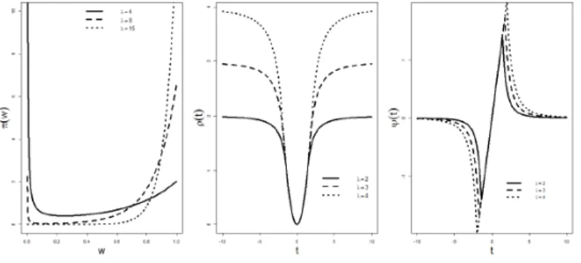
There is a Bayesian understanding of the PAWLS model in (4.3). Suppose we have independent prior distributions: β0 ∝ 1, π(βj) ∝ e−λ10|βj| for 1 ≤ j ≤ p, and
π(wi) ∝ (wi)−1e−λ20|1−wi|I(0 < wi ≤ 1) for 1 ≤ i ≤ n, where I(·) is the indicator
function. The joint posterior distribution of the parameters,
π(β,w|y)∝ n
Y
i=1 exp−w2i(yi−x0iβ) 2−λ 20|1−wi| pY
j=1 exp{−λ10|β|j}.Thus the PAWLS estimation (β,ˆ w)b in (4.3) withλ1n=λ10/(2n)and λ2n=λ20/(2n) is equivalent to a corresponding posterior mode of β and w. In the left panel of Figure 3, we plot three sample curves of π(wi) for λ20 = 4,8,15. It is observed that, wi = 1 with a large probability for a large λ20, and wi = 0 with a large probability
for a small λ20. The convexity of π(wi)between0and 1justifies the outlier detection
4.2.1 A general threshold rule and its link to sparse M-estimation
In fact, the PAWLS with Lasso in (4.3) can be generalized to a series of weight shrinkage estimation which enjoys strong robustness. To understand this property, we first define a class of scaleshrinkage rule as follows.
Definition 4.1. (Scale Threshold Function) For any threshold parameter λ > 0, a positive functionΘλ(t), t ∈Ris defined to be a scale threshold function if it satisfies
(1) (Symmetric) Θλ(t) = Θλ(−t) ,
(2) (Non-increasing)Θλ(t)≥Θλ(t0) for 0≤t ≤t0 and
(3) (Two extremes) lim
t→0Θλ(t) = 1 and tlim→∞Θλ(t) = 0.
The scale threshold function in Definition 4.1 shares the similar spirit as one in [SO12], but these two types threshold functions have different features. Specifically, Θλ(·)here is designed to shrink any small positive values (close to 0) to 1, while the
one in [SO12] is to shrink any large values to0. Based upon the above scale shrinkage rule, we can establish an interesting connection between the PAWLS estimation and the sparse M-estimation. Such a connection explains strong robustness properties of the proposed PAWLS in (4.3).
Theorem 4.2. Suppose β˜ = ˜β(0,w)˜ is a solution in (4.2) for λ1n = 0 and we 2
i =
Θλ(yi−xiβ),˜ 1≤i≤n. Here Θλ(·) for someλ >0 is a threshold function defined in
Definition 4.1. Then β˜ is also an M-estimator such that β˜ = arg min
β
{Pn
i=1ρλ(yi − x0iβ)}. In particular, ψλ(t) = dρλdt(t) satisfies,
Figure 3. Display of Some Functions. Left: The Shape of πλ(wi) Function with
λ= 4,8,15; Middle: Theρλ Function with Tuning Parameterλ= 2,3,4; Right: The
ψλ Function with Tuning Parameter λ = 2,3,4
The proof of Theorem 4.2 is given in Appendix. Theorem 4.2 tells us that a weight generated from any given scale threshold rule can be linked to a corresponding M-estimator. For example, the PAWLS with the Lasso in (4.3) indicates that wˆi = {nλ2n/(yi−x0iβ)ˆ2} ∧1. Thus, if we let λ = nλ2n, then the scale shrinkage rule for
(4.3) becomes Θλ(t) = λ2/t4 if t2 > λ, 1 if t2 ≤λ. (4.5)
Thus from Theorem 4.2, the PAWLS estimation in (4.3) is linked to a corresponding sparse M-estimator with ψ function with
ψλ(t) = λ2/t3 if t2 > λ, t if t2 ≤λ, (4.6)
and the corresponding ρ function, ρλ(t) = −λ2/(2t2) +λ, if t2 > λ, t2/2, if t2 ≤λ. (4.7)
See the left and right panels in Figure 3 for three curves of ρλ(t) and ψλ(t) under
λ = 2,3,4. Notice that lim
t→∞ψλ(t) = 0 and tlim→∞ρλ(t) = λ. Thus the ρ function in (4.7) gives a weakly redescending M estimation with strong robustness. Naturally, the PAWLS solution in (4.3) can be understand as a regularized robust M-estimator with the Lasso penalty. From now on, our investigation is focused on this particular PAWLS estimator. Without being addressed in particular, the Lasso penalty is used in the PAWLS approach.
4.3 Implementation
4.3.1 Coordinate decent Algorithm for PAWLS
We first notice that (4.3) is not a convex optimization problem. This is not surpris-ing due to the link to a regularized redescendsurpris-ing M estimator and strong robustness discussed in Section 4.2.1. However, for a given w, the function of β is a convex optimization problem, and the vice versa. Therefore, the objective function (4.3) is a bi-convex function. This biconvexity guarantees that the algorithm has promising convergence properties [GPK07]. We can compute a PAWLS estimate efficiently in Algorithm 1 using coordinate decent algorithm [GPK07].
For each pair of(λ1n, λ2n), those initialization valuesβ(1),w(1)play important roles
during alterative iterative process. We suggest to use a multiple iterative strategy as follows: (1) when updating β, we start from β(1) =0 and w(1) = ˆw(λ
e
λ2n is an ideal tuning parameter searched from the last tuning parameter selection
process to be represented in the next section; (2) when updating w, we start from w(1) =1 andβ(1) =β(eˆ λ
1n, λ2n), where eλ1nis an ideal tuning parameter from the last tuning parameter selection process. Thus, initial values are improved for multiple times, and β(k) and w(k) are alteratively updated until converge.
Algorithm 1The PAWLS under fixed λ1n and λ2n
Given X∈Rn×p,y∈
Rn and λ1n, λ2n in a fine grid,
letλ1j =λ1n for1≤j ≤p, let λ2i =λ2n for 1≤i≤n
letk = 1 and obtain an initial β(k), w(k), and r(k) =y−Xβ While not converged do
[update β] cj =n−1X 0 jw(k) 0 wXj, zj =n−1X 0 jw(k) 0 wr+cjβ (k) j βj(k+1) =S(zj, λ1j)1/cj r=r−X0j(β(k+1)−β(k)) [update w] if r2 i > nλ2i, w (k+1) i ←nλ2i/r2i; otherwise w (k+1) i ←1 converged ifkβ(k+1)−β(k)k ∞ < and kw(k+1)−w(k)k∞ < k←k+ 1 end while deliver βˆ=β(k) and wb =w(k)
4.3.2 Tuning parameter selection
Like many other penalized regression, the selection of tuning parameters plays an important role in producing a well-behaved PAWLS estimate. Due to the high computation efficiency of Bayesian Information Criterion (BIC) [S+78], we choose two
optimal tuning parameters λopt1n and λopt2n by modifying BIC as follows, BIC(λ1n, λ2n) = nlog ( n X i=1 ˆ w2i(λ1n, λ2n)(yi−x0iβ(λˆ 1n, λ2n))2+ p n+p ) +bs(λ1n, λ2n) log(n), (4.8) where bs(λ1n, λ2n) = sb1 +bs2 with bs1 = 1 + #{1 ≤ j ≤ p : ˆβj(λ1n, λ2n) 6= 0} and b
s2 = #{1 ≤ i ≤ n : ˆwi(λ1n, λ2n) < 1}. Here bs1 and sb2 are the estimated number of nonzero regression coefficients and and outliers, respectively. Different from the classical BIC, we include a term n+pp in the first part in (4.8) dealing with the possible blowup. This may happen if a very small λ1n is used such that all wbis are close to 0. The optimal tuning parameters are search alternatively by minimizing BIC in (4.8) from a fine grid of λ1n, λ2n. We first fix λ∗1n and find an “ideal” λ∗2n using BIC;
then this λ∗2n is fixed, and we continue to search an “ideal” λ∗1n by minimizing the BIC. The same procedure is repeated iteratively until an optimal pair (λopt1n, λopt2n) is obtained. This alternative search has high computation efficiency and performs well in our numerical studies.
Remark 2: We suggest to search for λ2n first since a well chosen λ∗2n (for outlier
screening) at the beginning can reduce the estimation damage caused by outliers dur-ing the iteration process significantly. This is also verified by our limited numerical experience.
Remark 3: We discard those (λ1n, λ2n) such that bs2/n ≥ r, where r can be any value larger than 0.5. This is reasonable since any single linear regression model will be invalid for if a data has more than 50% outliers. In this case, subgroup analysis should be applied. In our numerical studies, we takes r = 0.8. In fact, we have also
tried different values between r = 0.5 to 0.8. All worked very well and improved the efficiency of the tuning parameter selection process significantly.
4.3.3 Improve the PAWLS using the adaptive penalty
Since the adaptive Lasso in general has better variable selection properties than the Lasso [Zou06, HMZ08], we also consider the PAWLS with the adaptive Lasso penalty by minimizing 1 2n n X i=1 w2i(yi−x0iβ) 2+λ 1n p X j=1 |βj|/|β (0) j |+λ2n n X i=1 |1−wi|/|1−w (0) i |, (4.9)
where w(0)i and βj(0) are two initial estimates ofwi and βj, respectively. The
compu-tation of (4.9) is similar to Algorithm 1 by replacing λ1j byλ1n/|β
(0) j | for 1≤ j ≤p and λ2i by λ2n/|1−w (0) i | for 1≤i ≤n. By convention, w (0) i = min{w (0) i ,0.999} and
βj(0) = min{βj(0),0.001}. If all 0 ≤ wi(0) < 1 and βj(0) for 1 ≤ j ≤ p are the same, respectively, then (4.9) becomes the PAWLS in (4.3).
As we know, a estimation consistent initials need to be applied in order to have an variable selection consistent adaptive Lasso estimator [Zou06, HHM08]. From those non-asymptotic properties investigated in Section 4.4, the PAWLS-Lasso estimates are reasonable choices for βj(0) and w(0)i in (4.9). This is also demonstrated in our numerical studies to be presented in the next section.
From our empirical experiences, the above procedure of works very well in all our numerical studies in the next section.
4.4 Non-asymptotic Properties
In this section, we will investigate the estimation properties of the PAWLS in ultra high-dimensional settings when p = O(exp(nα)) for some 0 ≤ α < 1. To simplify
the presentation, we omit the intercept in model (4.1) in this section. All proofs are given in Appendix.
For notation’s convenience, we replaceνi = 1−wi for1≤i≤nin some scenarios
and assume all covariates to be standardized such that Pn
i=1x 2
ij = n, 1 ≤ j ≤ n
in this section. We put all weights and covariates coefficients together and denote a n+p dimensional unknown parameters vector θ = (θ01, θ20)0, where θ1 = (β1,· · · , βp)0
with true values θ∗1 = β∗ and θ2 = (λ2n/λ1n)(ν1,· · · , νn)0 with true values θ2∗ = (λ2n/λ1n)w∗. Here w∗ = (w∗1,· · · , wn∗)
0. Let S
10 = {1 ≤ j ≤ p : βj∗ 6= 0} with
the cardinal value s1 = |S10|, S20 = {1 ≤ i ≤ n : w∗i < 1} with the cardinal value
s2 = |S20|, and J0 = {1≤ k ≤n+p, θk∗ 6= 0} be the true active set for θ∗ with the cardinal value |J0|s1+s2 =s. We also denotean= min
1≤i≤S20
wi∗.
We consider the fixed design such that |xij| ≤bn for all iand j and the following
assumptions.
(A1): i =w∗iηi are i.i.d. sub-Gaussian distribution with mean0and scale factor
σ >0. (A2): (i) sbn n1/2 =o(1); (ii) slog(n) na2 n =o(1).
(A3): there exists a constant M >0 such that max
j∈S10
RE(s, c): For some integer s, such that 1 ≤ s ≤ p+n, and a positive c, the following restricted eigenvalue condition holds:
κ(s, c) = min d6=0 kdJ c 0k1≤ckdJ0k1 |J0|≤s kΨ1/2dk2 kdJ0k2 >0, (4.10)
wherek · kq is the`q norm,d = (d01,d 0 2) 0 and Ψ= 1 n X0X 0 0 σ2ω∗−2 withω ∗ being a diagonal matrix generated from w∗.
From (A1), the standard deviation of yi, σyi = σ/w∗i → ∞ if wi∗ → 0 for i ∈
S20. Thus (A1) relaxes the normal assumption on random error in PLS regression dramatically. (A3) is a trivial condition on nonzero regression coefficients. A2(i-ii) indicate that the total number of non-zero βj∗s and outliers cannot grow with n too fast. It also meansancan not decay to 0 too fast. If bothanandbnare constants, then
(ii) is redundant. The RE(s, c) condition mimics the restricted eigenvalue condition (3.1) of [BRT09].
Consider the following three events regarding the random error ,
• A1 ={k0Xk∞< nλ1n/4}; • A2 ={max 1≤i≤n 2 i/w ∗ i < nλ2n/4};
• A3 = {k0Dν˜Xk∞ < nλ1n/4}, where Dν˜ is a diagonal matrix consists of any estimation ν˜= (˜ν1,· · · ,ν˜n)0.
Lemma 4.3. On event A1∩A2∩A3,
kθˆ−θ∗k1 ≤4kθˆJ0 −θ
∗
J0k1 (4.11)
Lemma 4.4. Under (A1), we have
P(Ac1)≤2pe− nλ2 1 32σ2 (4.12a) P(Ac2)≤2nexp −nλ2na 2 n 8σ2 (4.12b) P(Ac3)≤2 exp −M0min nλ4 1n 256K2σ4, nλ2 1n 16Kσ2 , (4.12c) where K = sup q≥1 q−1 E 21/σ2q1/q
andM1 >0is an absolute constant. In particular, if we choose λ1n ≥σ(c1)1/2(ln(p)/n)1/2 for c1 >32, then
P(Ac1)≤2p−c1/32 →0 when p→ ∞.
If we choose λ2n≥σ2c2log(n)/(na2n) for some c2 >8, then
P(Ac2)≤2n1−c2/8 →0 when n→ ∞.
For the above λ1n,
P(Ac3)≤O exp −c1M0log(p) 16K min c1log(p) 16Kn ,1 .
Thus if p=O(exp(nα)) for α >0, then P(
Ac3)→0 for α ≥1/2.
Lemma 4.3 provides an upper bound of the PAWLS estimator under three events. Lemma 4.4 investigates the lower probability bounds for the occurrence of those events. We now develop the theoretical properties of the proposed PAWLS estimator. In particular, we expect to obtain some non-asymptotic oracle inequalities for both
ˆ
w and β.ˆ
Theorem 4.5. Suppose A1 and RE(s,3) hold. Then with probability at least 1−
P5 k=1hi, we have kθˆJ0 −θ ∗ J0k1 ≤ 8λ1ns κ(s,3)2 and kθˆJ0 −θ ∗ J0k2 ≤ 8λ1ns1/2 κ(s,3)2 , Here h1 = 2pnexp −nλ 2 1n 32σ2 , h2 = 2nexp −nλ2na 2 n 8σ2 ,
h3 = 2 exp −M0min{ nλ 4 1n 256K2σ4, nλ2 1n 16Kσ2} with K = sup q≥1 1 q E 2 1 σ2 q1/q
and M1 >0 is an absolute constant,
h4 = 48σ κ(s,3) λ1n(1 + log(2n))1/2 λ2n s1/2 ann1/2 , h5 = 384σ k2(s,3) λ1n(1 + log(2n))1/2 λ2n sbn nan .
In particular, if (A2) and (A3) hold and λ1n/λ2n ≤ O(1), then h4 =o(1) and h5 = o(1) .
Theorem 4.5 gives the oracle inequalities of joint estimators ofθ. Those properties are similar to ones for the PLS estimator (with the Lasso penalty) of β only when w∗ is given in advance. When w is jointly estimated with β, the non-asymptotic properties for bothβˆandwˆ can be obtained by letting two regularization parameters λ1n and λ2n changes with n dependently such that λ1n/λ2n =O(1).
The following corollary provides an explicit, shared rate of λ1n and λ2n such that
both βˆ and wˆ are estimation consistent even though p grows with n at an almost exponential rate. This is a direct result from Lemma 4.4 and Theorem 4.5.
Corollary 4.6. Suppose p = O(exp(nα)) for 1/2 < α < 1 and all assumptions in
Theorem 4.5 hold except that A2(ii) is replaced by s=o n(1−α)/2. If we can choose λ1n ≥σ(c1)1/2(ln(p)/n)1/2 for c1 >32, and λ2n ≥σ2c2log(n)/(na2n) for some c2 >8
such that λ1n =λ2n, then with probability at least 1−2p1−c1/32−2n1−c2/8, we have kβˆS10 −β ∗ S10k1+kwˆS20−w ∗ S20k1 ≤ 8λ1ns κ(s,3)2 and kβˆS10−β ∗ S10k2 +kwˆS20 −w ∗ S20k2 ≤ 8√2λ1ns1/2 κ(s,3)2 . 4.5 Numerical Result
In this section, we demonstrate the performance of the PAWLS using both simu-lation studies and real data analysis under two settings: p < n and pn.
4.5.1 Simulation studies
In all our simulation studies, the data are generated from the mean shift model without an intercept:
yi =x0iβ+γi+i, i= 1,· · · , n,
where xis are simulated independently from a multivariate normal distribution with
mean 0 and variance C= (0.5|j−k|)
p×p. All simulations are repeated for 100 times.
Apparently, the true mean shift model is a misspecified model for our weighted regression model setting in (4.1). However, we will demonstrate that the advantage of the PAWLS are still obvious compared with other methods from simulation studies.
Example 4.7. (Low-dimensional case) We choose n = 50, p = 8, and set β∗ = (3,2,1.5,0,0,0,0,0)0. The random error i and the mean shift parameter γi
are generated under the following four cases.
Case A: i ∼N(0,22), and γi = 0 for i= 1,· · · , n ;
Case B: i follows a t distribution with degrees of freedom of 2, and γi = 0 for
i= 1,· · · , n;
Case C: similar to Case A, except that γi = (−1)I(U1<1/2)(20 + 10U2) for 1 ≤ i≤n/10, whereU1 and U2 are independent U[0,1].
Case D: similar to Case C, except that 10is added on all xijs for 1≤i≤n/10
and 4≤j ≤8.
Case A includes only normal data; Case B includes heavy tails errors; Case C includes normal data with outliers in y direction; while Case D includes outliers in bothx and y directions.
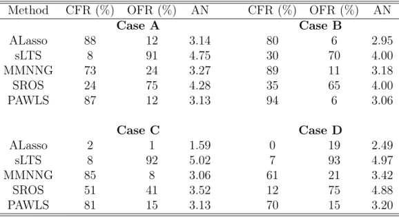
We compare the performance of the PAWLS with the adaptive Lasso in terms of both variable selection and outlier detection with the PLS with the adaptive Lasso (ALasso: [Zou06]) and several other sparse robust estimation mentioned in Section 1 including the SROS, MMNNG, and sparse LTS (sLTS). As a fair comparison, the adaptive Lasso penalty are used in all methods except for MMNNG where a nonneg-ative garrote method is used. The codes of both the MMNNG and sLTS are public available. The code of the SROS is provided by authors. The computation of the ALasso is the same as the PAWLS by fixing allwi = 1.
fitting the model (CFR) and over-fitting the model (OFR) are computed. The average model size (AN: mean of #{1 ≤ j ≤ p : ˆβj 6= 0}) is also reported. All those
results are summarized in Table 2. Our simulation results also show that the PAWLS outperforms all other estimators in terms of variable selection in almost all cases. In particular, we have those findings. (1) The ALasso performs the best as expected when the data is normal in Case A; But the PAWLS is most comparable with the ALasso, compared with all other robust estimation. (2) When the data is heavy tailed in Case B, the ALasso behaves much worse than some of other sparse robust estimates. Among them, the PAWLS performs the best, while both the sLTS and SROS perform badly in this case. (3) When some normal data are contaminated in Case C, the ALasso loses its efficiency completely, while the PAWLS still performs quite well and beats all other robust methods. (4) When outliers exist in bothx and y directions, the PAWLS also performs the best.
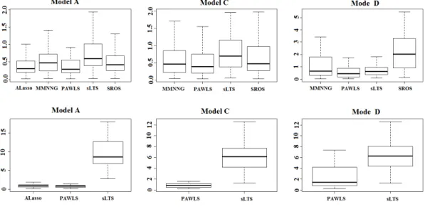
We also evaluate the coefficients estimation using the mean squared error (MSE),
kβˆ−βk2 out of all repetitions. Those results of MSE (after removing 10% of largest ones) from Case A, C and D are plotted in Figure 4. The boxplot under Case B shows the similar pattern as ones from C and D and is omitted here. It is observed that PAWLS has the best estimation efficiency by providing the smallest MSE results among all methods when the data are contaminated.
To evaluate the outlier detection performance, we compute the mean masking probability (M: fraction of undetected true outliers), the mean swamping probability (S: fraction of non-outliers labeled as outliers), and the joint outlier detection rate (JD: fraction of repetitions with 0 masking) out of all repetitions. The higher JD is, the better; the smaller M and S are, the better. Since the ALasso, MMNNG
and SROS are not designed to specify outliers, we only report the outlier detection results from the PAWLS and sLTS in Table 3. It is observed that the sLTS turns to produce a very large swamping probability in most cases. Compared with the sLTS, the PAWLS has a much better outlier detection performance.
In summary, the PAWLS is robust when the data is contaminated and does not lose much efficiency as other robust methods in normal case. Besides the PAWLS, the MMNNG performs the second best. However, compared with the PAWLS, the MMNNG is much more expensive in computation. In addition, MMNNG does not produce the outlier detection result.
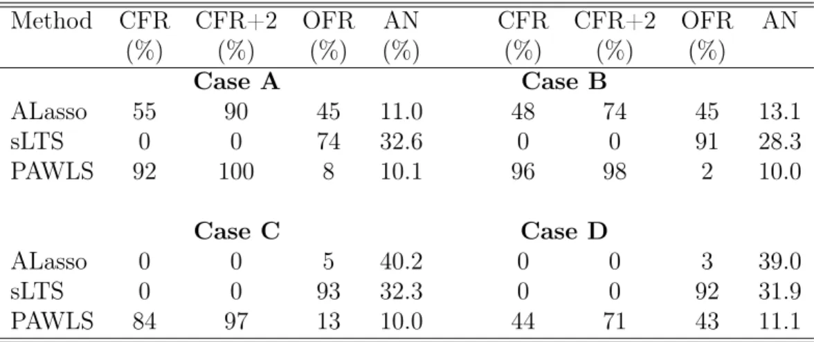
Table 2. Variable Selection Results for Example 1 (β = (3,2,1.5,0,0,0,0,0)0)
Method CFR (%) OFR (%) AN CFR (%) OFR (%) AN
Case A Case B ALasso 88 12 3.14 80 6 2.95 sLTS 8 91 4.75 30 70 4.00 MMNNG 73 24 3.27 89 11 3.18 SROS 24 75 4.28 35 65 4.00 PAWLS 87 12 3.13 94 6 3.06 Case C Case D ALasso 2 1 1.59 0 19 2.49 sLTS 8 92 5.02 7 93 4.97 MMNNG 85 8 3.06 61 21 3.42 SROS 51 41 3.52 12 75 4.88 PAWLS 81 15 3.13 70 15 3.20
Figure 4. Boxplot of MSE in Example 1. The first row: Example 1 (Case A, C and D from the left to right); The second row: Example 2 (Case A, C and D from the left to the right). ALasso results are omitted in Case C and D since the MSE values are very large compared with others in those cases.
Table 3. Outlier Detection Evaluation in Example 1 and 2
sLTS PAWLS Model M (%) S (%) JD(%) M (%) S (%) JD(%) Example 1 Case A 0 5.30 100 0 1.22 100 Case B 0 9.92 100 0 4.22 100 Case C 0 1.87 100 0 0.67 100 Case D 0.4 1.89 99 0 0.44 100 Example 2 Case A 0 20.8 100 0 0.07 100 Case B 0 18.5 100 0 1.15 100 Case C 0 12.9 100 0.8 0.18 98 Case D 0.1 13.0 99 27.8 0.08 100
Example 4.8. (high-dimensional case) Similar to Example 1, except that n = 100, p = 500 and β = (2010,00p−10)0, where ck is a k-dimensional vector consists of all
c.
In this example, we can only compare the PAWLS with the sLTS and ALasso since all other methods are only designed for p < n. We tried to implement their approaches in high-dimension where p > n, but failed.
All variable selection results are reported in Table 4. Besides OFR, CFR and AN reported in Example 1, we also report the OFR+2, the ratio of correct-fitted model and over-fitted model with at most two extra variables. Outlier detection results are reported in Table 3. Some of MSE results are reported in those Boxplots in Figure 4. It is observed that the advantages of the PAWLS is even more obvious is high-dimensional settings, regarding variable selection, outlier detection and robust estimation. The PAWLS produces much higher CFR and CFR+2 than both the ALasso and the sLTS in contaminated cases. In this setting, sLTS turns to generate over-fitted model in most cases. When the data is normal, the PAWLS still works very well by producing high CFR value.
4.5.2 Real data applications
The two datasets introduced in 1.3 will be studied in this section: Air pollution data (p < n) and NTC-60 data (p > n).
4.5.2.1 Air pollution
As mentioned earlier, observation 21 had to be removed since it contains two missing values, resulting in n = 59 and p = 14 in our study. We also consider the logarithm transformation on the pollution variables, due to their skewness. In
addition, both the covariates and response variables are scaled to have median value of zero and MAD (median absolute deviation from the median) value of one. This procedure keeps all variables within a comparable range level.
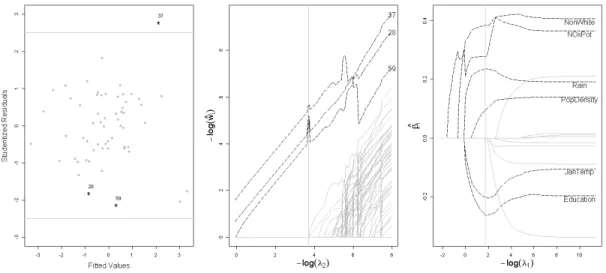
[GV15] analyzed the data with a QQ-plot and reveals the possible contamination of the data set. The PAWLS estimates ofβ are compared with output from four other methods in Table 5. The PAWLS selects 7 variables from 14 of them. Among them, Rain, PopDensity, NonWhite, and SO2Pot are positively correlated with the log-value of the mortality rate, and JanTemp, Education, and HCPot have the negative effect. It is worthwhile to point it out that JanTemp is selected by all four robust methods, but not by ALasso. For this data, the PAWLS produces similar results as ones from MMNNG and SROS. However, the last two does not produce outlier detection results. This comparison is also consistent with the simulation studies, where MMNNG performs the second best after the PAWLS.
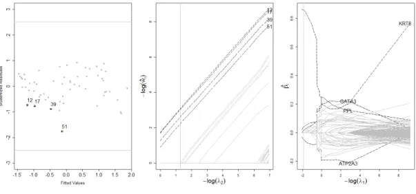
The outlier detection results from the PAWLS are reported in Figure 5, where three suspected outliers detected by the PAWLS are highlighted by “*”. See the studentized residual plot in the left panel Figure 5. These three potential outliers are observation 28 from Lancaster, PA, observation 37 from New Orleans, LA, and observation 59 from York, PA. It is observed that the last two observations are masked using studentized residuals with cutoff value 2.5.
We also plot the solution paths of βˆjs along a sequence of λ1n. See the right panel
in Figure 5. The solution paths ofwˆis along a sequence ofλ2nis also plotted in middle
panel. Instead of being removed from the regression analysis completely, those two potential outliers are still used, but with some wˆi value being much smaller than 1,
![Figure 1. Estimation Picture for (a) The Lasso and (b) Ridge Regression [Tib96]](https://thumb-us.123doks.com/thumbv2/123dok_us/1441075.2692980/18.918.205.821.389.981/figure-estimation-picture-lasso-b-ridge-regression-tib.webp)
![Figure 2. Graphic Representation of A Few Examples of M-estimators [Zha]](https://thumb-us.123doks.com/thumbv2/123dok_us/1441075.2692980/27.918.262.708.705.984/figure-graphic-representation-examples-m-estimators-zha.webp)