Beyond linear similarity function learning

(1)

Beyond Linear Similarity Function

Learning

Julien Bohn´e

A dissertation submitted in partial fulfillment of the requirements for the degree of

Doctor of Philosophy of

University College London.

Department of Computer Science University College London

(2)

(3)

3

I, Julien Bohn´e, confirm that the work presented in this thesis is my own. Where information has been derived from other sources, I confirm that this has been indicated in the work.

(4)

(5)

Abstract

Being able to measure the similarity between two patterns is an underlying task in many machine learning and data mining applications. However, handcrafting an effective similarity function for a specific application is difficult and tedious. This observation has led to the emergence of the topic of similarity function learning in the machine learning community. It consists in designing algorithms that automatically learn a sim-ilarity function from a set of labeled data. In this thesis, we explore advanced simsim-ilarity function concepts: local metric, deep metric learning and computing similarity with data uncertainty.

Linear metric learning is a widely used methodology to learn a similarity function from a set of similar/dissimilar example pairs. Using a single linear metric may be a too restrictive assumption when handling heterogeneous datasets. Lately, local metric learning methods have been introduced to overcome this limitation. However, most methods are subject to constraints preventing their usage in many applications. For example, some require the knowledge of all possible class labels during training. In this thesis, we present a novel local metric learning method, which overcomes some limitations of previous approaches.

Deep learning has become a major topic in machine learning. Over the last few years, it has been successfully applied to various machine learning tasks such as clas-sification or regression. In this thesis, we illustrate how neural networks can be used to learn similarity functions which surpass linear and local metric learning methods.

Often, similarity functions have to deal with noisy feature vectors. In this con-text, standard similarity learning methods may result in unsatisfactory performance. In this thesis, we propose a method which leverages additional information on the noise magnitude to outperform standard methods.

(6)

(7)

Acknowledgements

I would like first to thank my supervisor, Massimiliano Pontil, for his precious advises and his patience. This PhD has been supported by a company named Safran Identity & Security and I want to thank St´ephane Gentric, the head of face recognition research, for his time and our fruitful discussions.

I am also immensely grateful to my wife, V´eronique, for being the source of count-less moments of happiness and supporting me in hard times.

(8)

(9)

List of Figures

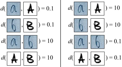
1 What a good similarity function is depends on the task of interest. On left side,d(·,·)would be a desirable distance for letter recognition. On the right side, it would be a suitable distance for writing style comparison. 20

2 Face verification process . . . 21

3 Border crossing using face recognition . . . 21

2.1 Samples from MNIST digits . . . 37

2.2 Images from LFW . . . 38

2.3 Images from FRGC . . . 39

3.1 `_γ,b(r,z)withγ =0.5 . . . 44

3.2 Performance comparison between the hinge loss and the linear loss on FRGC . . . 44

3.3 On FRGC, using tough dissimilar pairs improve performance at low false positive rates. . . 47

3.4 Performance of hinge loss-based loss functions on FRGC. . . 49

3.5 Performance of hinge loss-based loss functions on LFW. . . 50

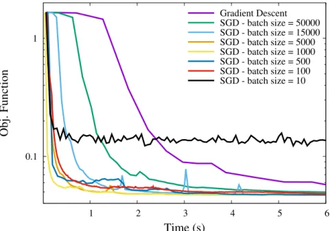
3.6 Speed of convergence of Gradient Descent and SGD function of the batch size. . . 55

4.1 Percentiles of Bhattacharyya distance between neighbors function of the embedding dimensionalitym. . . 66

4.2 Synthetic data with small mean angle difference between the 3 GMM components. Left: Examples of positive pairs (points linked by black segments). Right: Performance of the Euclidean Distance, Global Met-ric and Local MetMet-ric. . . 68

(14)

14 List of Figures

4.3 Synthetic data with large mean angle difference between the 3 GMM components. Left: Examples of positive pairs (points linked by black segments). Right: Performance of the Euclidean Distance, Global Met-ric and Local MetMet-ric. . . 69 4.4 Optimizing both the matrices M0..K and the GMM parameters θ

im-proves performance on the synthetic dataset. . . 70 4.5 Impact ofKon LMLML’s performance on MNIST. . . 71 4.6 Performance of LMLML and other methods on FRGC . . . 72 4.7 Each row shows the images with the highest posterior probability

P(k|x)for a specifick. . . 73

5.1 DET curve of LMLML and Deep Metric on FRGC. The red curve cor-responds to the performance withK=3 which is the value giving the best results on FRGC. . . 83 5.2 DET curve on MNIST for LMLML and Deep Metric. . . 84 5.3 These two pairs of digits are considered to be very similar by Deep

Metric but not by LMLML. Deep Metric handles similar pairs of fea-ture vectors which are too far away in the original feafea-ture space better than local metrics. . . 85 6.1 Graphical representation of the generative model using plate notation.

All the covariance matricesS_µ, S_w andS_c_,_i are considered fixed in the generative model. However, while the matrices Sc,i are provided by UA-PPCA or the feature extractor, the matricesS_µandS_ware estimated by the EM algorithm. . . 94 6.2 Examples of digits with three levels of additional noise: none (left),

medium (middle) and strong (right) . . . 98 6.3 High resolution (left) and low resolution (right) versions of an FRGC

image . . . 101 6.4 Histograms of the magnitude of a high frequency Gabor filter response

on LR and HR images . . . 102 6.5 Examples of occluded faces . . . 103 6.6 Original (left) and frontalized version (right) of an image from MUCT . 105

(15)

List of Figures 15

6.7 Masks associated with 3 of the 5 bins of yaw angle. The proportions of discarded pixels (hatched areas) are written in white. . . 105

(16)

(17)

List of Tables

3.1 Classification Accuracy of hinge loss-based loss functions on MNIST

and Reuters . . . 49

3.2 Regularizer Comparison on Public Datasets. Performances indicated are Classification Accuracy for MNIST and Reuters, Accuracy for LFW and FNR at FPR=0.1% for FRGC. . . 52

3.3 Metric Learning for face verification with identity document photos. Comparison of the False Negative Rate at 0.1% of False Negative Rate. 53 4.1 Classification Rates . . . 71

4.2 Accuracy on LFW. . . 74

5.1 Network configurations. In the Activation function column, MO stands for maxout. . . 83

5.2 Classification Rates . . . 83

6.1 EER on MNIST . . . 99

6.2 Sensitivity to the uncertainty accuracy . . . 99

6.3 EER on MNIST with strong noise function of the dimensionality re-duction method used for training (rows) and how the low dimensional projection is performed (columns) . . . 100

6.4 FNR at FPR=0.1% on FRGC depending on the training set and test set resolutions . . . 102

6.5 Impact of occlusion on the FNR at FPR=0.1% on FRGC . . . 104

6.6 Robustness to pose variations. FNR at FPR=0.1% on two databases with large variations in pose. . . 106

(18)

(19)

Introduction

Pattern recognition tasks, such as clustering or nearest-neighbor classification, require computing similarity between pairs of data points. The overall task performance strongly depends on how well the similarity measure accurately reflects the actual prox-imity between the concepts represented by those points.

For many pattern recognition tasks the processing pipeline starts with a feature extraction step during which the raw data (e.g. images, speech signal, health moni-toring) are transformed into feature vectors of fixed length. In this work, we focus on similarity functions for feature vectors inRn. In this setting, a similarity function is a function f :_Rn×_Rn_7→

R which outputs small values for pairs of similar inputs and larger values for dissimilar ones. In this thesis, in an abuse of terms we usesimilarity functionto denote both similarity and dissimilarity functions (such as distances).

Whatsimilarmeans is entirely application dependent. For example, to obtain good performance in letter classification using a nearest-neighbor approach, the similarity between two images depicting the same letter should be high and it should be low for pairs of images of different letters. Alternatively, if the goal is to differentiate writing styles, the similarity measure should be completely different (See Figure 1). The Euclidean distance and other non-parametric similarity functions usually fail to deliver good performances because they ignore both the variable relevance of each feature for the task and the dependencies among those features.

Handcrafting a similarity function for a specific task may be complex and requires sophisticated prior knowledge of both the data and the task. However, it is often more effective and efficient to automatically learn the similarity function from a set of labeled data. Labels can be the class to which each data point belongs to, but several similarity function learning methods use a weaker form of supervision. They only need to be provided with a set of data pairs labeled similar when the two points belong to the

(20)

20 Introduction

d( , ) = 0.1

d( , ) = 10

d(

,

) = 10

d( , ) = 10

d( , ) = 0.1

Figure 1:What a good similarity function is depends on the task of interest. On left side,d(·,·)

would be a desirable distance for letter recognition. On the right side, it would be a suitable distance for writing style comparison.

same class, ordissimilarwhen then do not. It is also popular to use triplets instead of pairs, each triplet containing two data points of the same class and a third point from a different class.

Learning a similarity function is a difficult task. Compared to other machine learn-ing tasks, such as classification or regression, the need to consider the data points by pairs is a source of complexity as it belies the common assumption that training points are independent and identically distributed. Moreover, the number of parameters to learn grows quadratically with n. This tends to make similarity learning algorithms slower and relatively prone to over-fitting.

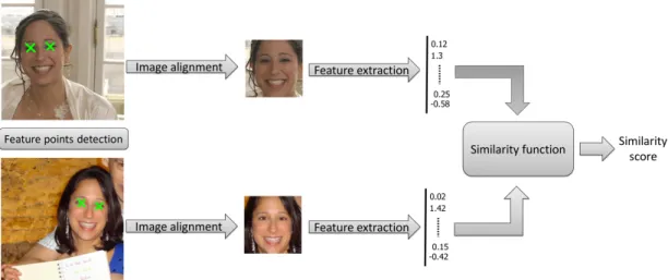
Similarity function learning has been a topic of interest in machine learning for many years but its popularity has increased recently when one of its most prominent applications, namely, face verification, became a central topic in computer vision. Face verification could be decomposed into three steps (see Figure 2). First, each face is detected and aligned (usually by finding a geometric transformation which puts points such as eyes, mouth corners etc. at specific locations). Second, the aligned image is transformed into a feature vector by applying filter banks, computing histograms of gradients etc. Then, a similarity score can be computed between pairs of feature vectors. To obtain the best overall performance, a good similarity function must be used and this is the topic of this thesis.

(21)

Introduction 21

Figure 2:Face verification process

Figure 3:Border crossing using face recognition

designing biometric identification systems. For example, it provides automatic solu-tions based on face recognition to check at the border that a passport holder is its right-ful owner (see Figure 3).

In Chapter 1, we give a general presentation about similarity functions and briefly describe the most popular methods. In Chapter 2, we describe the datasets used in this thesis to assess the performance of similarity functions. The training of most similarity function learning methods consists in optimizing an objective function. We discuss the components of such functions and related optimization methods in Chapter 3. Linear metrics obtain good results on a large variety of scenarios but are sometimes too simple to deal with heterogeneous data. Local metric learning is one of the type of methods

(22)

22 Introduction

which have been introduced to overcome this limitation. We present a novel local metric learning method in Chapter 4. Deep Learning is a strong trend in Machine Learning. It is widely used to perform classification but can also be used to compute similarities. Chapter 5 describes how to create a similarity function based on the Deep Learning principles. Uncertainty is a central issue in machine learning because the features we work with are often corrupted by noise. In Chapter 6, we introduce a new similarity function which takes advantage of information on the uncertainty of the features of each data point. Finally, we conclude this thesis by exposing the future challenges in similarity function learning.

(23)

Notation

We introduce here notations which are used throughout this thesis. Notation Description

x_i Data point in_Rn

y_i Class ofx_i

r_{i j} Similar/dissimilar pair indicator, r_{i j} =1 if y_i=y_j and−1 other-wise

Sn+ The set of positive definite matrices of sizen

S Set of similar pairs,(i,j)∈ S =⇒ r_{i j}=1 D Set of dissimilar pairs,(i,j)∈ D =⇒ r_{i j}=−1 T Set of training pairs,T =S ∪ D

k · kF Frobenius norm

Tr(·) Trace of a matrix

[z]+ Positive part operator:[z]+=max(0,z)

N(· |µ,S) Probability distribution function of the multivariate Normal

(24)

(25)

Chapter 1

Background

This chapter presents the different types of similarity functions and the most prominent methods to learn their parameters. Metric, or distance, is a popular class of similarity functions. We first give its definition and then describe the state-of-the-art algorithms to train a type of parametric distance called Mahalanobis distance. In the last section of this chapter, we extend our presentation to non-distance similarity functions.

1.1 Definition of a Metric

A metric over a setAis a functiond:A × A 7→_R+ which satisfies 3 properties: 1. Symmetry: ∀a,b∈ A, d(a,b) =d(b,a),

2. Identity: d(a,b) =0 ⇐⇒ a=b,

3. Triangular inequality: ∀a,b,c∈ A,d(a,b) +d(b,c)≥d(a,c).

The Minkowski distance of order pis defined in _Rn by(∑n_k₌₁|a_k−b_k|p₎1/p

wherea_k

andb_kare respectively thekth component ofaandb. This family includes many of the usual non-parametric distances such as the Euclidean distance (p=2), the Manhattan distance (p=1) or the Chebyshev distance (p=∞). Minkowski distances of order p with p<1 are not metrics as they do not satisfy the triangular inequality, they might nonetheless be effective similarity functions for some applications.

Non-parametric distances cannot be adapted to take into account the specificities of the data and the task of interest. Therefore, they give poor results in practice when all features are not equally relevant for the task. Parametric similarity functions have been developed to overcome this limitation. In the remaining part of this chapter, we present the most popular types of similarity functions and the algorithms which have been proposed to learn their parameters.

(26)

26 Chapter 1. Background

1.2 Mahalanobis Distance

Originally, the Mahalanobis distance [1] has been introduced to deal with features of different scales and potentially correlated. The Mahalanobis distance between x_i

and xj in Rn is defined by

q

(xi−xj)>S−1(xi−xj)where S is an estimate of the co-variance matrix of the data. By an abuse of language in the metric learning com-munity, Mahalanobis distance is generally used to denote any distance of the form

d_M(x_i,x_j) =

q

(x_i−x_j)>M(x_i−x_j) whereM ∈_Sn

+, the cone of positive-semidefinite

(PSD) matrices of sizen. WhenMis not positive-definite, the Mahalanobis distance is not a distance but only apseudo-distancebecause it does not satisfy the 2nd property but only weaker one which is xi =xj =⇒ d(xi,xj) =0. Many metric learning algo-rithms have been proposed to find an appropriate matrixM given a set of labeled data, several are presented below.

Any PSD matrix M can be factorized as M =L>L with L∈_Rn×n. So, a Ma-halanobis distance parametrized by M can be written as the Euclidean distance after applying the linear transformation L to the data: d_M2(x_i,x_j) = (x_i−x_j)>M(x_i−x_j) = (Lxi−Lxj)>(Lxi−Lxj). This equivalence is very useful to speed-up distance com-putation when each data point is compared to many others. Instead of computing

q

(xi−xj)>M(xi−xj)for each pair, the linear transform is applied once per data point and Mahalanobis distances are replaced by Euclidean distance which is much faster. Some metric learning methods aim to find the best matrixM, whereas others try to find

Ldirectly. To further speed-up the distance computation and also reduce the memory needed to store the feature vectors, it can be interesting to reduce the feature vector dimensionality. Discriminative dimensionality reduction can be achieved by searching for a rectangular matrix L∈_Rr×n withr<n, such that the Euclidean distance in the reduced space is a good similarity function.

A popular choice for the matrix M comes from assuming that all classes fol-low multivariate Normal distributions and share the same covariance matrix [2]. This within-class covariance matrix is generally approximated by the within-class scatter matrix Sw= 1 C C

∑

c=1 1 n_c nc

∑

i=1 xc,i− 1 n_c nc

∑

j=1 xc,j > xc,i− 1 n_c nc

∑

j=1 xc,j (1.1) whereCis the number of classes in the training set andn_cthe number of data points in

(27)

1.2. Mahalanobis Distance 27

thecth class. The probability that two data pointsx_iandx_j in_Rnboth belong to a class whose center is xi+₂xj is equal to

N xi x_i+x_j 2 ,Sw N xj x_i+x_j 2 ,Sw = exp ₋₍_xi−xj₎>_S−1 w (xi−xj) 4 2πdet(Sw)n (1.2)

where N(· |µ,S) is the probability distribution function of the multivariate Normal

distribution of meanµand covarianceS. Using the Mahalanobis distance withM=S−_w1

is equivalent to using the above probability as a similarity function.

There is a tight link between using a Mahalanobis withM =S−_w1 and the multi-dimensional Linear Discriminant Analysis (LDA) [3] which is a discriminative dimen-sionality reduction method. In several algorithms, such as FisherFace [4], the similarity function used is the Euclidean distance in the post-LDA subspace. The LDA finds a lin-ear subspace which simultaneously maximizes the scattering of the class centers while making the classes as compact as possible. It leads to the optimization of the Fisher’s criterion:

max L∈Rm×n

det L>S_bL

det L>S_wL (1.3)

whereS_w is the within-class scatter matrix defined above and S_b is the scatter matrix of the class centers. The Fisher’s criterion is invariant with regards to the norm of the columns ofLwhereas those norms have an impact on the performance of the Eu-clidean distance in the post-LDA subspace. The most common method to maximize the Fisher’s criterion is to use the matrix whose columns are the generalized eigenvec-tors corresponding to themlargest eigenvalues inS_bl=λSwl. The resulting matrixL satisfies the equationL>S_wL=I which is equivalent toM=L>L=S−_w1 whenm=n

(no dimensionality reduction). The between-class scatter matrixS_bhas an impact only when the number of dimensions is effectively reduced:m<n.

The Mahalanobis distance withM=S−_w1only uses the within-class scatter matrix and discards all information about between-class variations. K¨ostinger et al. propose to use both with KISSME (Keep It Simple and Straightforward MEtric) [5]. This method takes as inputs a set of similar pairs and a set of dissimilar ones, respectively denoted S and D, and assumes that feature vector differences of similar and dissimilar pairs follow 0-mean multivariate Normal distributions. The covariance matrices of those

(28)

distributions, respectively denotedS_wandS_b, are simply estimated by the empirical co-variance matrices of the feature vector differences of the corresponding pair set. When the data follows a statistical model, the likelihood ratio test is known to achieve the minimal error rate to choose between two mutually exclusive hypotheses (Neyman-Pearson lemma). We are interested in finding out if the difference between two feature vectors comes from a similar or a dissimilar pair, so we look at the likelihood ratio

P(xi−xj|dis)

P(xi−xj|sim). Given the Gaussian assumption presented above, the log-likelihood ra-tio is equal to(x_i−x_j)> S−_s1−S−_d1(x_i−x_j) up to a constant. To obtain the closest pseudo-metric to this log-likelihood ratio, the authors takeM = S−_s 1−S−_d1

+ where

(·)+ is the projection on the PSD cone operator.

Many metric learning algorithms are not based on a statistical modeling of the data but directly optimize an empirical objective function. The first method which has formulated metric learning this way is Mahalanobis Metric for Clustering (MMC) [6]. The matrixMis found by solving the following optimization problem:

max M

∑

(i,j)∈D d_M(x_i−x_j) (1.4) s.t.

_∑

(i,j)∈S d_M2(xi−xj)≤1 (1.5) M0. (1.6)

The optimization is performed by projected gradient ascent. After each gradient step, the matrixMis alternatively projected on the set of matrices satisfying each constraint until both are satisfied. The problem is convex and the procedure is therefore guaran-teed to converge to the global optimum. This optimization method requires numerous eigenvalue decompositions of the matrixM and hence becomes rather slow when the dimensionality of the feature space increases.

Large Margin Nearest Neighbor (LMNN) [7] has been designed to improve near-est neighbor classification using a set of labeled points(x_i,y_i). The first step is to build a similar pair setS by selecting for each point thek-nearest neighbors of its class with the Euclidean distance. The second step is to optimize a cost function which gives a penalty when the squared distance of a similar pair (xi,xj) is larger than the squared distance betweenx_iand any pointx_k belonging to a different class. To prevent infinite

(29)

1.2. Mahalanobis Distance 29

space inflation, the cost function also penalizes the sum of squared distances of similar pairs. More specifically, the cost function is given by

min M∈Sn+₍_i_,

∑

_j₎_∈_S d_M(x_i−x_j) +c

_∑

(i,j,k) yi=yj yi6=yk 1+d_M(x_i−x_j)−d_M(x_i−x_k) + (1.7)

where[·]+ =max(0,·) andc is a positive constant set by cross-validation. This

opti-mization problem is convex and close to the standard SVM for classification problem. The authors propose an efficient optimization algorithm which takes advantage of the fact that most of the triplets (xi,xj,xk)do not create any penalty. Several extensions of this work have been introduced to deal with multi-tasks learning [8], nonlinear pro-jections [9] or local metrics [10]. More details about the latter are given in the next section.

In Logistic Discriminative Metric Learning (LDML) [11], the authors propose to cast the metric learning problem into a log-likelihood maximization. The squared Mahalanobis distance is transformed into the probability that the two points be-long to the same class using a sigmoid function: pi j = P yi=yj|xi,xj;M,b

= 1+exp d_M(x_i,x_j)−b−1 wherebis a bias term. The log-likelihood of the dataset is

∑

(i,j)∈S lnp_{i j}+

_∑

(i,j)∈D ln(1−p_{i j}) (1.8)

and is maximized with respect toMandbusing a simple gradient ascent. This problem being concave, the optimization is guaranteed to converge to the global maximum.

Like with most machine learning tasks, over-fitting is a key issue in metric learn-ing. Several articles propose a regularized objective function to limit over-fittlearn-ing. In Information Theoretic Metric Learning (ITML) [12], the regularization is performed by penalizing the LogDet divergence betweenMand a given matrixM₀which can be, for example, the identity matrix or the inverse of the sample covariance matrix. The cost function favors matricesM for which similar pair distances are below a given upper boundu∈_R+ _{and dissimilar pair distances are above a given lower bound}_`_∈

R+: min M∈Sn+,ξ ₍_i_,

∑

_j₎_∈_S ξi j u +log ξi j u +

_∑

(i,j)∈D ξi j ` +log ξi j ` +λd`d(M,M0) (1.9)

(30)

s.t. d_M2(xi,xj)≤ξi j ∀(i,j)∈ S (1.10)

d_M2(xi,xj)≥ξi j ∀(i,j)∈ D (1.11)

where d_`_d(M,M₀) =Tr MM₀−1−log det MM₀−1−n is the LogDet divergence be-tween two matrices andλ controls the strength of the regularization. This optimization

problem is convex and the authors present an algorithm based on Bergman projections to solve it. There is no need to enforce the positive semi-definiteness ofMspecifically as this is automatically taken care of by the regularization term becaused_`_d(M,M₀) =∞ ifM andM0 do not share the same range. A kernelized version and an online version of the algorithm are also proposed in [12].

Several results exist on generalization error bounds for metric learning. In [13], Jin et al. use uniform stability to show that, under some assumptions, a regularizer bound-ing Tr(M)improves robustness with high dimensional data. A trace norm regularizer is also used in BoostMetric [14], a method which builds the matrixMby incrementally adding rank-1 matrices in a way similar to what Adaboost does with weak learners. Nonetheless, Maurer advocates in [15] that trace norm regularization can lead to too sparse solutions and learning instability. On the other hand, he shows a generaliza-tion error bound based on Rademacher complexity which depends onkMk_F. A metric learning algorithm is derived from this observation, it combines a hinge loss-based empirical error and a penalization of the Frobenius norm of matrixM, namely

min M∈Sn+ ₍_i_,_j₎

∑

_∈_S_∪_D 1+ri j γ 1− d_M2(x_i,x_j) + +λkMkF (1.12)

whereγis the width the margin andλcontrols the regularization strength. More details

about this objective function are given in Section 3.1.2. The optimization problem (1.12) is solved via stochastic gradient descent (SGD).

1.3 Other Types of Similarity Functions

As seen in the previous section, Mahalanobis distance learning has been widely ad-dressed by the research community. However, other types of similarity function have also been explored. We present more complex function types in this section.

(31)

dis-1.3. Other Types of Similarity Functions 31

criminative information. For example, when data points are obtained by applying a bank of linear filters on an image, the norm varies strongly with the image brightness and contrast. Therefore, the norm is an irrelevant information for many similarity func-tion learning applicafunc-tions where invariance to such perturbafunc-tions is sought. The cosine similarityCS(x_i,x_j) = x>i xj

kxik2kxjk2 is often used to obtain norm-invariant similarity func-tions. Like the Euclidean distance, the cosine similarity can also be parametrized by a PSD matrixM to adapt to the data and task at hand:

CS_M(x_i,x_j) = x > i Mxj

x>_i Mx_ix>_jMx_j. (1.13)

Nguyen et al. apply this parametric cosine similarity to face verification [16]. They define the following objective function with respect to the linear data transformation matrixL

max

L

∑

(i,j)∈S∪D

r_{i j}CS_M(x_i,x_j) +λkL−L0k2F (1.14) whereM=L>L,L₀ is a predefined matrix and λ controls the strength of the

regular-ization. The regularization term is close in spirit to that of ITML. This optimization problem is not convex and there is no guarantee to reach the global maximum. The optimization procedure initializes the matrix L with L0 and then uses the conjugate gradient method.

The Joint Bayesian method [17] relies on Gaussian assumptions over both the class centers distribution and that of the samples within a class. More specifically, each data point is expressed asx_i=µyi+wi whereµyi corresponds to the center of the class yi andw_ito the variation with respect to this class center. Moreover,µyi is assumed to be drawn from the distributionN(· |0,S_µ)andw_ifromN(· |0,S_w). The authors describe a variational Expectation-Maximization (EM) algorithm to estimateS_µ andS_w from a set of labeled training points (xi,yi). Given the model, it is possible to compute the likelihood of any data points pair(x_i,x_j)considering that they belong to the same class (Hsim) and the likelihood considering that they belong to different classes (Hdis). The authors propose to use the log-likelihood ratio

llr(xi,xj) =log

P x_i,x_j|H_sim;S_µ,S_w P x_i,x_j|H_dis;S_µ,S_w

!

(32)

as similarity function. Thanks to the Gaussian assumptions, the log-likelihood ratio has a simple expressionllr(x_i,x_j) =x>_i M₁x_j+x>_i M₂x_i+x>_jM₂x_j+const whereM₁andM₂

are two PSD matrices which are computed from S_µ and S_w. Other articles [18, 19] find the parameters of analogous similarity functions by optimizing hinge-loss based objective functions.

Using kernels is a common way to extend linear machine learning meth-ods into non-linear ones [20] which has been popularized by SVMs. A non-linear similarity function can be created by combining a non-non-linear mapping Φ : Rn 7→ F with a Mahalanobis distance in the feature space F: dM2F(xi,xj) = Φ(x_i)−Φ(x_j)>M_F Φ(x_i)−Φ(x_j). However, the feature space F can be very high or even infinite-dimensional, making it costly or impossible to explicitly compute the mappingΦ. The kernel trick allows to implicitly make calculations in the feature space without actually performing the mapping. To make this possible we need to define a kernelK:_Rn×_Rn_7→

Rwhich corresponds to an inner product in the feature space F. Conveniently, the Mercer’s theorem states that any functions fulfilling the Mercer’s condition is an inner product in some feature space. Nonetheless, it is not trivial to kernelize an algorithm as it requires expressing all operations on data points as inner products. The LDA presented in the previous section is one of the first methods which have be kernelized [21]. A non-linear version of ITML using kernels has also been proposed by its authors [12].

As we have already seen, there is a strong connection between learning a simi-larity function and learning a data transformation such that a non-parametric simisimi-larity like the Euclidean distance delivers good performance. The idea of using neural net-works to perform the data transformation has first been explored in the 90’s for signa-ture verification [22] and more recently for face recognition with Convolutional Neural Network (CNN) [23, 24] or standard descriptor-based approaches [25, 26]. In all these methods, the weights of the neural network are obtained by minimizing an objective function similar to those used in ITML, LMNN, LDML, etc. The main differences are the inputs types (images or feature vectors) and the network structure.

Mahalanobis distance has been shown to be quite effective on various tasks but it suffers from a strong limitation: a single linear metric is used to compare data over all the input space. This may be inappropriate in order to handle heterogeneous data. This

(33)

1.3. Other Types of Similarity Functions 33

observation is the root of the development of local metric learning methods which adapt the dissimilarity function to the local specificities of the data. For illustrative purpose let us consider two examples. It is well known that in digit classification some digits are easily mistaken for another such as “1” and “7” or “3” and “8”. It seems therefore reasonable to focus on different features to discriminate digits in the “1-7” region and in the “3-8” one in order to reduce the number of misclassifications. Our second example is face verification: should we put the emphasis on the very same features to compare two pictures of Caucasian males and two pictures of Asian females? Weinberger and Saul proposed an extension of LMNN to local metric (MM-LMNN [10]), in which a specific metric is associated to each class and all metrics are jointly learned to optimize a classification criterion. KISSME [5] has also been extended to local metric in [27] where one KISSME metric is learned separately for each class. These class-specific metrics are averaged with a global one to limit the risk of over-fitting due to the fact that each metric might be learned using only a limited number of training samples. GLML [28] uses a local metric to optimize nearest neighbor classification using the class conditional probability distributions.

All these local metric learning methods suffer from the same drawback, namely they need enough training samples per class to estimate the metrics. Therefore, they cannot be employed directly in applications in which there is a large number of classes with only a few training data points in some classes. To overcome this problem, a local metric learning method is introduced in [29] based on finite a number of linear metrics named PLML. The number of metrics is different from the number of classes and hence the method can scale up to a larger number of classes. However, this method is specifically designed for nearest neighbors classification as it can only compute the similarity of pairs for which at least one data point is in the training set. This strongly limits the practical range of tasks that PLML can deal with. For example, it prevents the application of PLML to the problem of face verification. In Chapter 4, we introduce a method called LMLML which overcomes those limitations.

When several local metrics are learned, one issue is to determine how to compare data samples which come from different subparts of the input space. CLML [30] is an alternative to LMLML. It jointly learns many locally linear projections such that any pair of projected points can be effectively compared using Euclidean distance. Like

(34)

in LMLML, the input space is soft-partitioned using a GMM. More details about this partitioning are given in Section 4.1.

(35)

Chapter 2

Performance Evaluation

In the next chapters, we compare the performance of several similarity function learn-ing methods. We present here how we measure performances and the datasets on which those methods have been evaluated.

2.1 Performance Measures

In this section we present the performance measures we use to evaluate similarity func-tions in this thesis. A similarity function takes two inputs and outputs a score. There-fore, it is natural to evaluate it like a pair classifier with a DET curve that we define below. The process to obtain this curve is composed of four steps:

1. We compute similarity scores for a large number of pairs for which we know the correct labels (similar or dissimilar).

2. For every possible thresholdt, we compute the number false positive errors (dis-similar pairs dimmed (dis-similar by thresholding the (dis-similarity) and false negative errors (similar pairs dimmed dissimilar by thresholding the similarity).

3. Those error counts are transformed into rates by dividing them by the correspond-ing number of pairs to obtain a False Positive Rate (FPR) and a False Negative Rate (FNR) for every thresholdt.

4. We plot the FNR as a function of the FPR. This curve is called a Detection Error Tradeoff (DET) curve.

A DET curve displays the performance of a similarity function at all the possible op-erating points (thresholds) but for some applications, like face verification, people are often focused on performance at low FPR. To better visualize the performance at low FPR, a common practice is to plot the DET curve with the FPR axis in logarithmic

(36)

36 Chapter 2. Performance Evaluation

scale.

A DET curve gives of global view of the performance of a similarity function but it is sometimes convenient to synthesize the performance in one value to compare different methods easily. The Equal Error Rate (EER) is often used to this end. It is defined by EER=FNR(t)where the thresholdtis chosen so that FPR(t) =FNR(t). It is also common to compare methods by looking at the FNR at a given value of FPR. The chosen FPR depends on the operating point of interest for the target application.

Similarity functions are also used for classification tasks to improve performance of ak-nearest neighbor classifier. In this case, we usually measure the performance by looking at the classification accuracy which corresponds to the proportion of requests correctly classified.

2.2 Classification Datasets

Similarity function learning is often used as a means to improve nearest neighbors clas-sification. Indeed, some of the most famous metric learning methods such as LMNN [7] have been specifically designed for this problem. The five datasets we used for classification are described below.

2.2.1 MNIST

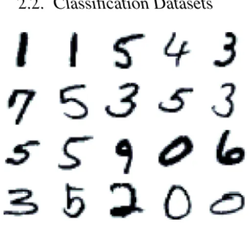
Handwritten digits classification has been widely used to assess the performance of similarity functions for classification. The MNIST dataset is composed of 70000 im-ages of size 28×28, 60000 for training and 10000 for testing. Figure 2.1 shows some examples of images composing the dataset. To create feature vectors, we do a PCA directly on the pixel values and 164 dimensions are kept after dimensionality reduction to retain 95% of the energy.

2.2.2 Isolet

Isolet is a spoken-letter datasets which contains 6238 vectors for training and 1559 for testing. 150 subjects were asked to pronounce each letter of the alphabet twice. The 617-dimensional feature vectors are composed of spectral coefficients, contour features, sonorant features, pre-sonorant features and post-sonorant features.

(37)

2.2. Classification Datasets 37

Figure 2.1:Samples from MNIST digits

2.2.3 Letter

Letter is a typed-letter recognition dataset. Distortions have been applied to the letters from 20 different fonts to create 20000 16-dimensional feature vectors composed of various statistical cues (mean, variance, correlation etc.) and edge count. The 16000 first samples are used for training and the remaining 4000 for testing.

2.2.4 Reuters

The text categorization dataset Reuters-21578 R52 consists of 9100 text documents which appeared on the Reuters newswire in 1987, 6532 in the training test and 2568 in the testing set. Each text belongs to one of the 52 topics and every topic has at least one text in the training set and one in the testing set. The classes are very unbalanced, some topics have more than 1000 text documents whereas others have just a few. Each text is described by a histogram of word occurrence spanning 5180 terms. A very large number of dimensions should be kept after the PCA to preserve 95% of the energy but to speed up the experiments we kept only the first 100 dimensions retaining 62% of the energy.

2.2.5 20newsgroup

20newsgroup is composed of 18774 messages taken from 20 Usenet newsgroups span-ning topics as diverse as alt.atheism or rec.motorcycles. Each text is represented by a 20000-dimensional word count histogram. The histograms are available for download on the Internet but each paper using this dataset proposes its own processing pipeline to transform those high dimensional histograms into more easily usable feature vec-tors (filtering with a stop-list, normalization, dimensionality reduction, etc.). We have implemented our own pipeline to create 1000-dimensional feature vectors.

(38)

38 Chapter 2. Performance Evaluation

Figure 2.2:Images from LFW

2.3 Face Verification Datasets

Face verification is an important and practical application of similarity function learn-ing. We present results on two face datasets: LFW and FRGC.

2.3.1 LFW

Labeled Faces in the Wild (LFW) [31] is a popular face verification dataset. It is com-posed of 13233 images of 5749 people taken from Yahoo! News in a wide range of acquisition conditions (pose, illumination, expression, age, etc.). Some examples are given in Figure 2.2. The best currently published results on LFW [24, 32] are obtained with deep learning methods trained on very large outside datasets (up to several mil-lions). In this thesis, we use an experimental setup where learning is performed on a small number of predefined training pairs (2700 similar and 2700 dissimilar) called re-stricted setting. We use a simple feature extractor which has been often used to assess performance of metric learning algorithms on LFW [16]. We start from the “aligned” images that we cropped to 150×80 to remove most of the background, then we ex-tracted descriptors composed of histograms of Local Binary Patterns [33] and finally we reduced their dimensionality to 300 by PCA.

2.3.2 FRGC

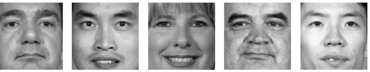
FRGC Experiment 1 [34] is a face dataset of 15000 images from more than 500 peo-ple. Figure 2.3 shows some examples. The pose of the subjects and the illumination have been controlled during the acquisition. Compared to datasets like Labeled Faces in the Wild presented above, this dataset is fairly simple. However, on this type of dataset, the interest is focused on the verification rate at low false positive rates (1% and below). This is a realistic setting for many security applications of face recognition (like smartphone unlocking or passport check at the border) where a false acceptance is a security breach and therefore should be very rare. After aligning the images using

(39)

2.3. Face Verification Datasets 39

Figure 2.3:Images from FRGC

the eyes locations, we computed UoCTTI HOG descriptors [35] extracted using the

VLFeat library [36] to obtain 6076-dimensional feature vectors. We then use PCA to reduce the dimensionality to 700.

(40)

(41)

Chapter 3

Objective Functions for Empirical

Loss Minimization

Similarity function learning methods can be classified into two categories. First, meth-ods based on a statistical model of the data (for example KISSME [5] or the Joint Bayesian Method [17]). Second, methods based on the optimization of an objective function which depends on a set of labeled training pairs (or triplets). This category in-cludes many of the most popular metric learning methods such as ITML [12] or LMNN [7]. This type of approach is often considered more flexible and more effective as it makes no assumption on the data distribution. In this chapter, we first describe the two components of objective functions: the empirical loss and the regularization term. The former drives the optimization toward a solution which performs well on the training set while the latter aims at limiting over-fitting to obtain good generalization performance. We conclude this chapter by presenting an optimization method based on Stochastic Gradient Descent.

3.1 Empirical Loss

3.1.1 Linear Loss

When the dataset is composed of similar and dissimilar pairs, the goal of the learning is to get small distances for similar pairs and large distances for dissimilar ones. A simple objective function has been proposed in [37], yielding to the optimization problem

min M∈Sn+₍_i_,

∑

_j₎_∈_T

(42)

42 Chapter 3. Objective Functions for Empirical Loss Minimization

s.t. kMkF ≤1 (3.1)

where r_{i j} is equal to 1 if (i,j) is a similar pair and -1 otherwise. The constraint on kMkF prevents that an increase of the scale ofM systematically leads to a lower cost whereas the loss should be intrinsically invariant to the scale ofM. The problem can be rewritten as max M∈Sn+ hM,Ai s.t. kMk2_F ≤1 (3.2) whereA=−∑(i,j)∈T ri j xi−xj

x_i−x_j> andh·,·i is the matrix inner product. We now prove that the solution to this problem is

M= A+ kA+kF

(3.3)

whereA₊ is the positive part of the matrixA.

LetM=Udiag(λ)U>andA=Vdiag(µ)V>be the eigendecompositions of

matri-cesMandArespectively. The two constraints onMboth depend only on its spectrum

λ: kMk2_F ≤1 ⇐⇒ ∑kλ_k2≤1 andM∈_Sn₊ ⇐⇒ ∀k∈ {1, . . . ,n},λk≥0. Moreover, ∀M∈_Rn×nandA∈_Rn×n, the inequalityhM,Ai ≤ hλ,µiholds and is tight if and only

ifU =V. Since we want to maximize hM,Ai and that the constraintkMk2

F ≤1 does not impactU, we can deduce thatU =V. We now need to solve

max λ n

∑

k=1 λkµk s.t. n

∑

k=1 λk≤1 ∀k∈ {1, . . . ,n},λk≥0. (3.4)

which has a trivial solution:

λk=

[µk]+

q

∑n_k0₌₁[µ_k]+2

(43)

3.1. Empirical Loss 43

The solution to the problem (3.2) is thereforeM=Vdiag(λ)V> which is equivalent to

M= _kA+kFA+ .

The weakness of the linear loss is that every pair equally contributes to the loss whereas some might carry more discriminative information than others. This explains the bad performance presented in the next section when compared, for example, to the hinge loss.

3.1.2 Hinge Loss

The hinge loss has been popularized by Support Vector Machine. As opposed to the linear loss, only the hard-to-classify training examples have an impact on the empirical loss. In the context of metric learning, we define our hinge loss by

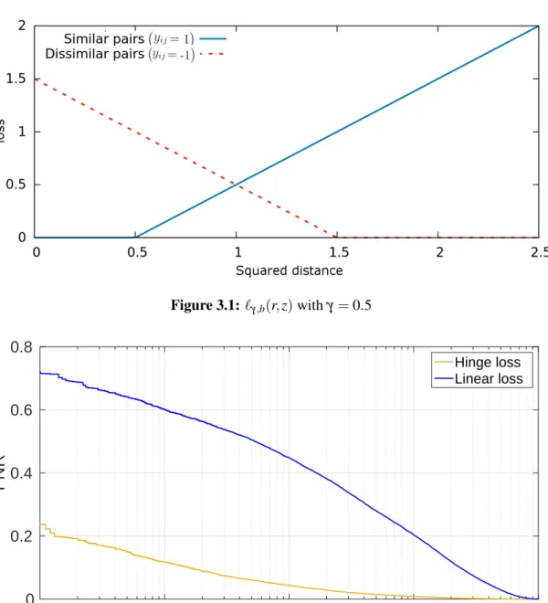
`_γ ri j,z = 1−ri j γ (1−z) + (3.6)

where γ corresponds to the margin width and z is a dissimilarity between xi and xj. The parameterγ is typically between 0.5 and 1: only the most difficult pairs impact the

objective function when γ is small but a larger proportion of them does ifγ is large.

Its optimal value depends on how helpful easy pairs are to improve the performance on the part of the DET curve we care about (low false positive or equal error rate for example). It also depends on the size of the training set: larger values of γ are better

with small training sets because when few pairs are available it is better not to discard too many of them even if they are not the most helpful ones. `_γ is plotted in Figure 3.1 for the two types of pairs. Equivalently, the hinge loss can be formulated with the help of slack variables and constraints:

`γ ri j,z =minξ s.t. z−γ+1<ξ ifri j =1 γ−z+1<ξ ifri j =−1 ξ ≥0. (3.7)

(44)

opti-44 Chapter 3. Objective Functions for Empirical Loss Minimization Figure 3.1:`γ,b(r,z)withγ=0.5

FPR

10-4 10-3 10-2 10-1 100

FNR

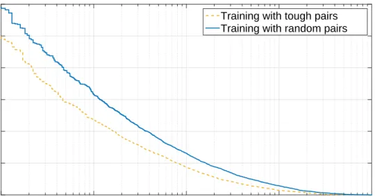
0 0.2 0.4 0.6 0.8 Hinge loss Linear loss

Figure 3.2:Performance comparison between the hinge loss and the linear loss on FRGC

mization problem: min M∈Sn+₍_i_,

∑

_j₎_∈_T `γ ri j,dM2(xi,xj) . (3.8)

The use of the hinge loss leads to better similarity functions than the linear loss presented in the previous subsection (see Figure 3.2). The hinge loss focuses on difficult pairs whereas the linear loss also tries to move pairs which are already well classified and therefore have no real impact on the performance.

For the classification task, many loss functions have been proposed in the liter-ature. The most frequently encountered are the exponential loss e

ri j

γ (1−d

2

(45)

3.1. Empirical Loss 45

in AdaBoost [38], and the logistic loss log

1+e ri j γ (1−d 2 M(xi,xj))

which comes from Logistic Regression. They can both be adapted to learn similarity functions and, be-ing convex losses, do not create specific optimization difficulties. Those different loss functions usually obtain similar accuracy but depending on the dataset some might be more effective than others. In this thesis, we only used the hinge loss because it has the advantage of being faster to compute.

3.1.3 Data Preprocessing

As it is common in similarity function learning, we apply a data preprocessing step. This step serves two purposes: first it reduces the dimensionality to speed up compu-tation for both training and testing, and second it reduces the noise thereby improving the overall performance of the algorithm.

As with most metric learning methods, we first center the dataset and reduce the dimensionality to an-dimensional space by PCA;nis often chosen so that 95% of the energy is preserved. We compute the within-class scatter matrix defined by

S=U

_∑

(i,j)∈S

(x_i−x_j)(x_i−x_j)>

!

U> (3.9)

whereU is the matrix formed by then leading eigenvectors of the covariance matrix of the data, and then multiply the data by S−1/2 to make the classes isotropic on av-erage. This transformation is known under different names such as mapping in the intra-personal subspacein face recognition [18] orWithin-Class Covariance Normal-ization (WCCN)in the speaker recognition community [2]. The transformed data points are nowx0=S−1/2U(x−m)wheremis the mean of the data. Like in [18], we finally rescale each feature vector so that it has a unit`2-norm.

3.1.4 Learning from Pairs or Triplets?

A similarity function takes a pair of input points and outputs a similarity value. It is therefore quite natural to learn the function parameters using pairs of inputs as it reflects how the function will actually be used. Usually, loss functions based on pairs generate a cost if a similar pair has a distance larger than a given threshold θs or a dissimilar one a distance smaller than a second threshold θd. It therefore leads to a similarity function which can effectively be thresholded to take decisions. This property

(46)

is very desirable for many applications, such as face verification for example. Some other similarity function learning methods use triplets of data points (x_i,x_j,x_k) with

y_i=y_j and y_i 6=y_k and their objective function penalize small or negative values of

d2(x_i,x_j)−d2(x_i,x_k). These objective functions are not primarily designed to create similarity functions whose output can be thresholded but rather functions designed to answer questions such as “Isx_imore similar tox_jthan tox_k?”. Triplets-based methods are therefore better suited for ranking applications (e.g. nearest neighbor classification) than pair verification. In this thesis, we focus on pairwise objective functions because we are interested in both ranking and thresholding.

3.1.5 Selecting Training Pairs from Class Labels

In many applications, training pairs are not provided but have to be built from labeled data points. The number of potential pairs grows quadratically with the number of training points, therefore it is often impracticable to use all of them because the train-ing would require a prohibitive amount of time. The choice of traintrain-ing pairs has a significant impact on the performance of the similarity functions learned.

When the similarity function is employed for nearest neighbors classification, it makes sense to pick training pairs composed of neighboring points because nearest neighbor classifiers base their decision only on such points. In this case, we propose proceeding as follow: for each data pointx, createksimilar pairs, formed byxand each of itskclosest neighbors from the same class, andk dissimilar pairs, formed byxand each of its k closest neighbors from a different class. This results in 2k training pairs per data point. We usek=5 in all our nearest neighbor classification experiments.

Similarity measures may also be thresholded to take a decision, as in face verifica-tion for example. The choice of the threshold leads to a specific trade-off between false positive and false negative rates. On datasets such as FRGC with few images per iden-tity, the number of potential similar pairs is limited and all of them can be used during training but a selection has to be made for the dissimilar ones. To learn a similarity function performing well at low false positive rates, the training set should include a large number of dissimilar pairs. To speed up the training, we use a simple hard dis-similar pairs mining scheme. We randomly pick a number of disdis-similar pairs equal to the number of similar pairs first and train our model with this set. We then compute the

(47)

3.2. Common Metric Learning Regularizers 47

FPR

10-4 10-3 10-2 10-1 100

FNR

0 0.05 0.1 0.15 0.2 0.25 0.3

Training with tough pairs Training with random pairs

Figure 3.3:On FRGC, using tough dissimilar pairs improve performance at low false positive

rates.

similarity for a large number of dissimilar pairs and select the 5 or 10% hardest pairs to train the similarity function again. This step could be repeated several times but in practice we observed little improvement after the first iteration. Figure 3.3 shows the improvement between learning the metric described in Section 3.1.2 with random and tough dissimilar pairs.

3.2 Common Metric Learning Regularizers

Over-fitting is often considered to be one of the main issues in machine learning. It occurs when the model to train is too complex, too powerful for the training data at our disposal. The consequence is that the learned model has a very low training error (error on the training data) but a high generalization error (error on unseen data). To limit over-fitting, one solution is to restrict the model complexity by limiting its number of parameters, for example using a low degree polynomial for curve fitting. The second possibility which offers more flexibility is to add a regularization term to the objective function. The regularizer penalizes complex models but they can nonetheless be chosen if the performance gain on the training set is large enough.

(48)

loss (3.6) and a regularizer can be formulated as

min M∈Sn+₍_i_,

∑

_j₎_∈_T

`γ ri j,dM2(xi,xj)

+λR(M) (3.10)

whereR(M)is the regularizer andλ is a meta-parameter controlling the regularization

strength which should be set by cross-validation. Several regularizers for metric learn-ing have been proposed in the literature. To provide an intuition about regularizer for metric learning, we rewrite the squared Mahalanobis distance using the eigendecom-positionM=U DU>: d_M2(x_i,x_j) = (x_i−x_j)>U DU>(x_i−x_j) (3.11) = n

∑

k=1 D_k_,_k x>_i U_·_,_k−x>_jU_·_,_k 2 (3.12)

whereD_k_,_k is the kth diagonal element ofD andU_·_,_k is the kth column ofU. We see that d_M2(x_i,x_j) is a weighted sum of squared differences along orthogonal directions, the weights being the eigenvalues of the matrixM. IfM has a very unbalanced spec-trum, the overall distance depends mostly on a few terms of the sum. On the contrary, if the spectrum ofM is flat, all terms contribute to d_M2(xi,xj)with comparable inten-sity. Domain specific knowledge can help to choose the suitable regularizer. If the discriminative information lies in a low dimensional subspace, then a regularizer favor-ing sparse spectrum should be chosen. Penalizfavor-ing the rank ofM leads to non-convex optimization problems. The common approach is to penalize the trace norm regularizer Tr(M)[13, 14] as it is the best convex approximation of the rank ofM. On the other hand, if there is a prior that no direction in the feature space should out-weight the oth-ers, a regularizer favoring a flat spectrum should be preferred. The regularizer is meant to balance the fact that the empirical cost only takes into account the directions which matter in the training set. The Frobenius norm of the matrixMis a simple convex reg-ularizer well suited in this case askMkF =

q

∑n_k₌₁Dk,k2. This assertion is supported by the fact that a generalization error bound function ofkMkF can be computed [15].

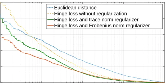
Figure 3.4, 3.5 and Table 3.1 show the performance on MNIST, Reuters, FRGC and LFW (see Chapter 2 for details about these datasets). We compare the Euclidean distance (M=I) with similarity functions learned without regularization and with the

(49)

3.2. Common Metric Learning Regularizers 49

Classification Accuracy

Method MNIST Reuters

Euclidean distance 96.61% 86.77%

Hinge loss without regularization 96.94% 88.02%

Hinge loss and trace norm regularizer 96.91% 88.04% Hinge loss and Frobenius norm regularizer 97.40% 88.64%

Table 3.1: Classification Accuracy of hinge loss-based loss functions on MNIST and Reuters

FPR

10-4 10-3 10-2 10-1 100

FNR

0 0.05 0.1 0.15 0.2 0.25 Euclidean distance

Hinge loss without regularization Hinge loss and trace norm regularizer Hinge loss and Frobenius norm regularizer

Figure 3.4:Performance of hinge loss-based loss functions on FRGC.

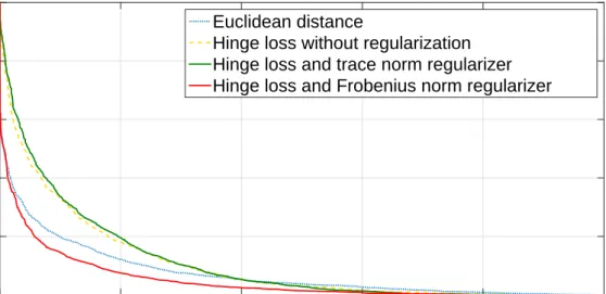
regularizers Tr(M)and kMkF. For all the datasets, we feed similarity functions with data preprocessed as described in Section 3.1.3. Therefore, the Euclidean distance in this new space is equivalent to the cosine similarity with M=S−_w1 in the original feature space. In our experiments, the discriminative information does not seem to be concentrated in a low-dimensional subspace and, therefore, the trace norm which induces too much sparsity in the spectrum ofMleads to a worse performance than the Frobenius norm. On LFW, MNIST and Reuters, the trace norm regularizer has even a negative impact on the performance and therefore very small values forλ are selected

by the cross-validation process. This explains why performance without regularization and with the trace norm regularizer are very close in Figure 3.5 and Table 3.1.

(50)

FPR

0 0.2 0.4 0.6 0.8 1

FNR

0 0.2 0.4 0.6 0.8 1 Euclidean distance

Hinge loss without regularization Hinge loss and trace norm regularizer Hinge loss and Frobenius norm regularizer

Figure 3.5: Performance of hinge loss-based loss functions on LFW.

3.3 A New Regularizer for Metric Learning

The Frobenius normkMkF is the most common regularizer in metric learning, it often leads to good results but is not always optimal. In particular, if prior information that Euclidean distance is already a good metric is available, the Frobenius norm might not be the best choice. This occurs, for example, when feature vectors are preprocessed with a method such as that described in Section 3.1.3 because it aims at getting good results with the Euclidean distance which is equivalent to usingM=I.

3.3.1 Regularizer

Ω

(

M

)

We introduce here a regularizer which favors matrices M close to a multiple of the identity matrix. Our objective function (4.4) is not scale-invariant as the threshold to decide whether two feature vectors are similar is set to 1. Therefore, multiplying the matrix by a factor should not be penalized. One could suggest to define the regularizer to beks×M−IkF wheresis a free variable introduced to accommodate for the scale of M and to optimizeM ands jointly during training. Unfortunately, this regularizer is not convex. Our proposal is to use Ω(M) =kM−sIkF. The two formulations are not equivalent. Ω(M)is scale invariant for diagonal matrices only. But in practice, as the goal of the regularizer is to favor matrices close the identity matrix and therefore diagonal, Ω(M) do not show a strong bias toward matrices with small coefficients as kMkF does.

(51)

3.3. A New Regularizer for Metric Learning 51

It is possible to avoid dealing explicitly with the additional variable s. Indeed, for any matrix M there is a closed-form solution for s which minimizes the regu-larizer. It is obtained by solving the equation ∂kM−sIkF/∂s= 0 which leads to

s=Tr(M)/n where n is the dimensionality of the feature space. The variable s can then be replaced by its expression to obtain a final formulation of our regularizer: Ω(M) =kM−Tr(_nM)IkF.

Ω(M)is convex as shown by the following proof:∀M,M0∈ Sn

+, Ω M+M0 2 = M+M0 2 − Tr(M+M0) 2n I (3.13) = 1 2 M−Tr(M) n I+M 0₋Tr(M0) n I (3.14) ≤ 1 2 M−Tr(M) n I +1 2 M0−Tr(M 0₎ n I (3.15) ≤ Ω(M) +Ω(M 0₎ 2 . (3.16)

The regularizerΩ(M) can easily be integrated into any gradient-based optimiza-tion scheme as its gradient has a simple closed-form:

∂Ω(M) ∂M =

M−Tr(_nM)I

Ω(M) . (3.17)

The regularizerkMkF favors matrices with small coefficients. When the parameter

λ which tunes the regularization strength is large, the use of kMkF tends to make all distances small and hence changes significantly the balance between similar and dissimilar pairs in the loss function. In extreme cases, only dissimilar pairs’ losses are active and similar pairs are completely ignored.

The RegularizerΩ(M)does not have this issue. It favors matrices which are close to any multiple of the identity but is not biased toward matrices with small diagonal elements. To get an insight about this, let’s study the gradient ofΩwhenMis a 2-by-2 matrix: M=    a c c b   . (3.18)

(52)

Table 3.2: Regularizer Comparison on Public Datasets. Performances indicated are

Classifica-tion Accuracy for MNIST and Reuters, Accuracy for LFW and FNR at FPR=0.1% for FRGC. MNIST Reuters LFW FRGC kMkF 97.77% 88.64% 87.77% 1.26% Ω(M) 97.86% 88.75% 87.60% 1.17% Relative error improvement -4.0% -1.0% +1.4% -7.1%

When minimizingΩ(M)with gradient descent, we easily see that, at the optimum, the off-diagonal element c will have a small absolute value and the diagonal elements a

andbare both going to be close to the average of their initial value. UsingΩ(M)as a regularizer for metric learning will not give more weight to the dissimilar pairs than to the similar ones even if the hyper-parameterλ is large.

The issue described above occurs frequently when a metric is learned to adapt features which have been learned for a specific dataset to a new one from a different domain which has few samples for training. We show the benefit of usingΩ(M)rather than Frobenius norm regularizer in a domain adaptation context in Section 3.3.2.

3.3.2 Effect of the Regularizer

Ω

(

M

)

In Section 3.3, we presented a new regularizer for metric learningΩ(M). We compare it to the most common metric learning regularizer, namely the Frobenius norm.

The performances reported in Table 3.2 correspond to the classification accuracy on MNIST and Reuters, accuracy on LFW and False Negative Rate at 0.1% of False Positive Rate on FRGC. Ω(M) improves performances on 3 out of 4 public datasets. The improvement is most significant on FRGC. This might be linked to the fact that the preprocessing stage described in Section 3.1.3 works particularly well on this dataset and hence constraining the matrixMto be close to the identity is effective.

We explained in Section 3.3 thatΩ(M)has an advantage over the Frobenius norm when the regularization strength hyper-parameterλ is large. Indeed, usingkMkF leads to giving more weight to the dissimilar pairs than the similar ones but our proposed regularizer does not. We illustrate this by performing the following face verification ex-periment. We use feature vectors produced by a Convolutional Neural Network (CNN)

(53)

3.4. Optimization 53

Table 3.3:Metric Learning for face verification with identity document photos. Comparison of

the False Negative Rate at 0.1% of False Negative Rate.

DB1 DB2 DB3 DB4 DB5 DB6 No Metric Learning 3.1% 4.7% 4.3% 4.0% 5.8% 17.3% ML withkMkF 3.3% 4.5% 4.4% 1.3% 5.4% 16.9% ML withΩ(M) 2.8% 4.0% 3.2% 1.2% 5.5% 16.2% Relative error improvement -15.1% -11.1% -27.3% -7.7% +1.9% -4.1%

trained on 500 000 images of actors downloaded from the Internet [39] and learn a metric to adapt those features to the kind of pictures used in identity documents.

For each regularizer, we learn a metric on 500 images and then evaluate it on 6 proprietary datasets made of photos from passports and other identity documents. Because of the few samples used for training, strong regularization is applied to pre-vent over-fitting. The different test datasets mainly differ by the type of acquisition process (use of a digital camera, old document scans etc.). We see in Table 3.3 that using Metric Learning improves performance on most of the datasets despite the small number of samples used for training. Ω(M) significantly outperforms the Frobenius norm on all but one dataset. The performance gap is larger in this experiment than on the public datasets; this is linked to the fact that the hyper-parameter λ (selected by

cross-validation) is much greater in this experiment.

3.4 Optimization

3.4.1 Stochastic Gradient Descent

Gradient Descent, also called Steepest Descent, is a standard and generic minimization technique. It starts with an initial solution and iteratively improves it by making a step in the opposite direction of the gradient of the function. Its most basic version uses a fixed step size which needs to be carefully tuned but various strategies have been proposed to speed-up the convergence.

Once the direction is chosen, finding the good step size is an optimization problem of its own calledline search. Many methods exist, one can use derivative-based meth-ods (1st and 2nd order), Golden Section Search [40] or approximate methmeth-ods such as

Beyond linear similarity function learning