Masters Theses Student Theses and Dissertations
Spring 2016
An IMU-based spacecraft navigation architecture using a robust
An IMU-based spacecraft navigation architecture using a robust
multi-sensor fault detection scheme
multi-sensor fault detection scheme
Samuel J. HaberbergerFollow this and additional works at: https://scholarsmine.mst.edu/masters_theses
Part of the Aerospace Engineering Commons
Department: Department:
Recommended Citation Recommended Citation
Haberberger, Samuel J., "An IMU-based spacecraft navigation architecture using a robust multi-sensor fault detection scheme" (2016). Masters Theses. 7505.
https://scholarsmine.mst.edu/masters_theses/7505
This thesis is brought to you by Scholars' Mine, a service of the Missouri S&T Library and Learning Resources. This work is protected by U. S. Copyright Law. Unauthorized use including reproduction for redistribution requires the permission of the copyright holder. For more information, please contact [email protected].
ROBUST MULTI-SENSOR FAULT DETECTION SCHEME
by
SAMUEL J. HABERBERGER
A THESIS
Presented to the Faculty of the Graduate School of the MISSOURI UNIVERSITY OF SCIENCE AND TECHNOLOGY
In Partial Fulfillment of the Requirements for the Degree
MASTER OF SCIENCE IN AEROSPACE ENGINEERING
2016 Approved by
Kyle DeMars, Advisor Henry Pernicka
ABSTRACT
Redundant sensor networks of inertial measurement units (IMUs) provide in-herent robustness and redundancy to a navigation solution obtained by dead reckon-ing the fused accelerations and angular velocities sensed by the IMU. However, IMUs have been known to experience faults risking catastrophic mission failure creating large financial setbacks and an increased risk of human safety. Different fusion meth-ods are analyzed for a multi-sensor network using cost effective IMUs, including direct averaging and covariance intersection. Simulations of a spacecraft in low Earth orbit are used to baseline a typical expensive IMU and compare the navigation solution obtained from a network of several low-cost IMUs from fused data. Robust on-board fault detection schemes are developed and analyzed for a multi-sensor distributed network specifically for IMUs.
Simulations of a spacecraft are used to baseline several cases of sensor failure in a distributed network undergoing fusion to produce an accurate navigation solution. The presented results exhibit a robust fault identification scheme that successfully removes a failing sensor from the fusion process while maintaining accurate navigation solutions. In the event of a temporary sensor failure, the fault detection algorithm recognizes the sensors’ return to nominal operating conditions and processes its sensor data accordingly.
ACKNOWLEDGMENTS
Firstly, I’d like to thank my advisor Dr. Kyle DeMars. You have given me the opportunity to envelop myself in the aerospace field of research, leaving me with a passion for navigation and estimation. You’ve held me to the highest expectations embedding me with a proud work ethic. Thank you for all of the priceless experience you have given me and for being a great advisor. I couldn’t have made it to this point in my academic career without your guidance and knowledge.
Secondly I’d like to thank my committee members Dr. Hank Pernicka and Dr. Serhat Hosder. As an undergraduate student, you have both instilled invaluable knowledge to me along with a contagious enthusiasm for academia via your classes and the satellite research team. My desire and aspirations of pursuing research in this field are greatly accredited to both of you.
My deepest appreciation goes to my loving and supportive family. Without you I couldn’t have made it to this point in my life and academic career. You have raised me with a work ethic that has given me the persistence, and will power needed in the engineering field. You will never know how truly thankful I am for all of the opportunities that you have provided for me.
Lastly, I’d like to thank my friends, classmates and academic peers James McCabe, Matthew Gualdoni, Jacob Darling, Levi Mallot, Matthew Glascock, John Schaefer, Keith LeGrand and the AREUS lab entity. I can’t thank you all enough for the knowledge and technical advice that has been provided to me from you. I couldn’t have asked for a better group of friends and academic peers to work with. It’s truly been a pleasure working and going to school with all of you.
TABLE OF CONTENTS Page ABSTRACT. . . iii ACKNOWLEDGMENTS . . . iv LIST OF ILLUSTRATIONS . . . ix LIST OF TABLES . . . xi NOMENCLATURE . . . xii SECTION 1 INTRODUCTION . . . 1 1.1 MOTIVATION . . . 3 1.2 OVERVIEW. . . 5 2 SPACECRAFT DYNAMICS . . . 7 2.1 IMU MODELING . . . 7
2.2 CONTINUOUS TIME DYNAMICS . . . 10
2.3 IMU INVERSION . . . 11
2.4 MULTI-SENSOR TRANSLATIONAL COMPENSATION . . . 13
2.5 DISCRETIZED DEAD-RECKONING EQUATIONS . . . 14
2.6 MEAN AND COVARIANCE PROPAGATION . . . 15
3 FUSION METHODOLOGY . . . 18
3.1 DIRECT AVERAGING . . . 18
3.2 COVARIANCE INTERSECTION . . . 20
3.2.2 Generalized Variance Weighting Selection . . . 25
3.3 FAULT TOLERANT FUSION . . . 26
3.4 FUSION EXAMPLE . . . 28
3.5 FUSION METHODOLOGY SUMMARY AND CONCLUSION . . . 31
4 FAULT DETECTION . . . 34
4.1 PRINCIPAL COMPONENT ANALYSIS . . . 34
4.2 FAULT DETECTION EXAMPLE . . . 37
4.3 MODIFIED PRINCIPAL COMPONENT ANALYSIS. . . 40
4.4 TRAINING VECTOR FAILURE . . . 43
4.4.1 Covariance Intersection in the Feature Plane . . . 43
4.4.2 Kullback-Leibler Divergence Covariance Threshold . . . 45
4.4.3 Shannon Entropy Threshold . . . 46
5 MEASUREMENT MODELING . . . 48
5.1 POSITION MEASUREMENT MODELING . . . 48
5.2 QUATERNION MEASUREMENT MODELING . . . 50
5.3 RANGE MODELING . . . 51
5.4 RANGE RATE MODELING . . . 53
5.5 UNIT VECTOR STAR CAMERA MODELING . . . 57
6 NAVIGATION ALGORITHM . . . 60
6.1 THE DISCRETE EXTENDED KALMAN FILTER . . . 60
6.1.1 Mean and Covariance Propagation . . . 60
6.1.2 Mean and Covariance Update . . . 64
6.1.4 Extended Kalman Filter Summary . . . 72
6.2 STATE ESTIMATE AND STATE ESTIMATION ERROR CO-VARIANCE PROPAGATION . . . 73
6.2.1 Position and Velocity Error Covariance . . . 74
6.2.2 Attitude Error Covariance . . . 79
6.2.3 Error Covariance in a Fusion Network . . . 81
6.3 MEASUREMENT PROCESSING . . . 83
6.3.1 Position Measurement . . . 83
6.3.2 Quaternion Measurement . . . 84
6.3.3 Range and Range Rate . . . 85
6.3.4 Unit Vector Star Camera . . . 86
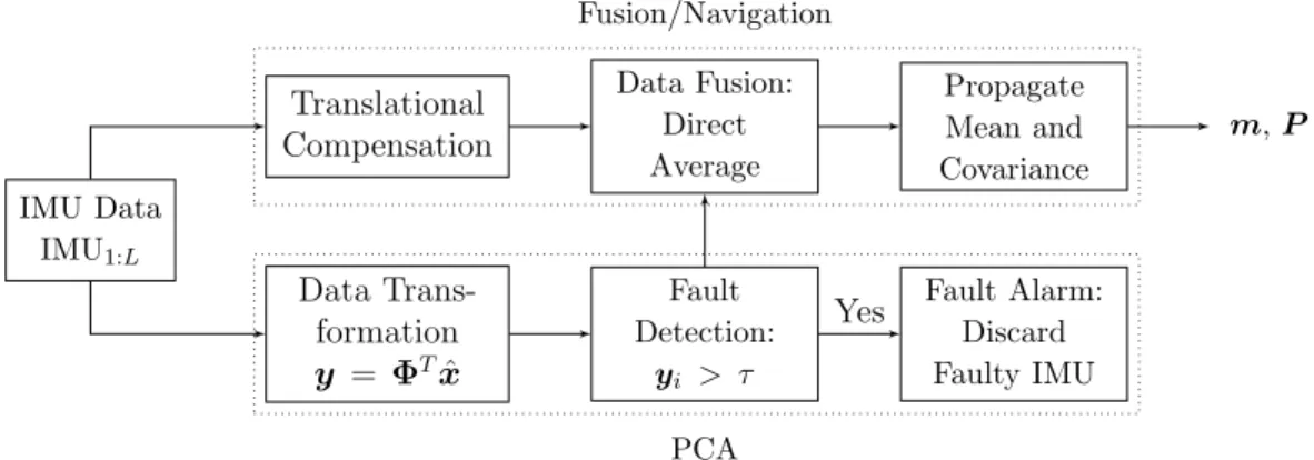
7 NAVIGATION/FAULT DETECTION SYSTEM ARCHITECTURE . . . 88
7.1 SYSTEM IMPLEMENTATION . . . 88
7.1.1 Fault Detection Architecture . . . 88
7.1.2 Fusion Architecture . . . 90
7.1.3 Navigation Architecture . . . 90
7.2 SENSOR CONFIGURATION . . . 91
8 SIMULATION RESULTS . . . 93
8.1 SIMULATION CONFIGURATION . . . 93
8.2 CASE 1: NOMINAL SENSOR OPERATION . . . 97
8.3 CASE 2: SINGLE SENSOR FAILURE . . . 104
8.4 CASE 3: MULTIPLE SENSOR FAILURES . . . 109
9 CONCLUSIONS . . . 118 9.1 FUTURE CONSIDERATIONS . . . 120 APPENDICES A IMU SPECIFICATIONS . . . 121 B FUSION ALGORITHM . . . 123 C MATRIX DEFINITIONS . . . 125
D MONTE CARLO ANALYSIS . . . 131
E EKF CONSIDERATION: UNDERWEIGHTING . . . 134
F ERROR PARAMETER SIMULATION RESULTS . . . 137
BIBLIOGRAPHY . . . 142
LIST OF ILLUSTRATIONS
Figure Page
1.1 x Position Standard Deviation versus Time with Plotted Errors. . . 4
2.1 IMU Errors vs. Time . . . 9
3.1 IMU Data Fusion Computed by Directly Averaging the Measurements . . . 19
3.2 Direct Averaging Fusion (N = 10,100 and 1000 Respectively) . . . 19
3.3 IMU Data Fusion Computed by Covariance Intersection . . . 24
3.4 CI Fusion Rule . . . 25
3.5 Position [m] and Attitude [deg] RSS Error . . . 30
3.6 x−y Uncertainty Contours [m] at 50, 200, 300 [s], Respectively . . . 31
3.7 Fusion Rule Uncertainty Comparison . . . 32
4.1 Effects of PCA Undergoing Single Sensor Failure for Static and Dynamic Systems . . . 38
4.2 First and Second Principal Components versus Time for a Static and Dynamic System Undergoing a Single Sensor Failure . . . 39
4.3 First and Second Principal Components Plotted Over 3-Dimensional Zero-Mean Data Set Before and After Failure . . . 40
7.1 Implementation Architecture Overview . . . 88
7.2 Fault Detection in a Static System. . . 89
7.3 Fault Detection in a Dynamic System . . . 90
7.4 IMU Data Fusion Computed by Directly Averaging the Measurements . . . 91
7.5 Navigation Architecture . . . 91
8.1 True Simulated Orbit Trajectory . . . 94
8.2 True Simulated ai ng and ωi/bi . . . 96
8.3 Time of Received Measurements . . . 96
8.4 Case 1: Position Standard Deviation/Errors and RSS vs. Time . . . 100
8.5 Case 1: Position Standard Deviation/Errors and RSS vs. Time . . . 101
8.6 Case 1: Attitude Standard Deviation/Errors and RSS vs. Time . . . 102
8.7 Case 1: Effects of MPCA with no Failures . . . 103
8.8 Case 1: Feature Plane CI Training Vector Fault Detection . . . 103
8.9 Case 2: Position Standard Deviation/Errors and RSS vs. Time . . . 105
8.10 Case 2: Velocity Standard Deviation/Errors and RSS vs. Time . . . 106
8.11 Case 2: Attitude Standard Deviation/Errors and RSS vs. Time . . . 107
8.12 Case 2: Effects of MPCA with a Single IMU Failure . . . 108
8.13 Case 2: Feature Plane CI Training Vector Fault Detection . . . 108
8.14 Case 3: Effects of MPCA with Multiple IMU Failures . . . 110
8.15 Case 3: Feature Plane CI Training Vector Fault Detection . . . 110
8.16 Case 4: Training Vector Failure using Only MPCA . . . 111
8.17 Case 4: Position Standard Deviation/Errors and RSS vs. Time . . . 113
8.18 Case 4: Velocity Standard Deviation/Errors and RSS vs. Time . . . 114
8.19 Case 4: Attitude Standard Deviation/Errors and RSS vs. Time . . . 115
8.20 Case 4: Effects of MPCA with a Training Vector Failure . . . 116
LIST OF TABLES
Table Page
3.1 Spacecraft IMU Configuration . . . 29 3.2 Fusion Example Legend . . . 29 8.1 Results Overview . . . 97
NOMENCLATURE
am,k Measured non-gravitational acceleration outputted from the
ac-celerometer
ωm,k Measured angular velocity outputted from the gyroscope
ˆ
n Estimated vector denoted by the hat ∆t Time step between measurements
∆ ˆv Measured non-gravitational acceleration multiplied by ∆t
∆ ˆθ Measured angular velocity multiplied by ∆t
¯
n Right handed, vector-first quaternion form ˆ rk Position estimate ˆ vk velocity estimate ˆ ¯ qk Quaternion estimate xk State of the system
mk Mean at some time k
Pk Covariance at some time k
σk Standard deviation at some time k Tbi Body to inertial attitude matrix
˜
n Fused solution
N Number of IMUs in system configuration
pg(x;m,P) Gaussian distribution in xwith a given mean and covariance Φ Feature plane mapping matrix
τ Fault alarm threshold
y Principal components
xT Training vector
Θ Parity space mapping matrix
vk External sensor noise at some time k δn state or measurement deviation
zk Received measurement at some time k
ˆ
zk Estimated measurements as a function of the mean at some time k
F Dynamics Jacobian
M Mapping matrix that maps the noise into the system dynamics
Q Process noise covariance matrix
ek State estimation error at some time k m−k Predicted mean at some time k m+k Corrected mean at some time k Pk− Predicted covariance at some time k Pk+ Corrected covariance at some time k
h(m+k) Estimated measurement as a function of the predicted mean
Wk Innovations or measurement residual covariance
Ck Cross covariance
Kk The Kalman gain
Spacecraft inertial measurement unit (IMU)-based navigation typically relies on a single, high-reliability, high-cost, tactical or strategic grade IMU to achieve accurate navigation solutions. In order to reduce cost while retaining accuracy of the navigation solution and improving the overall fault tolerance of the system, multiple lower-cost IMUs can be used. In order to combine the data from these multiple IMUs, several data fusion rules have been proposed. A direct averaging fusion rule of data from multiple IMUs was used in the demonstration and development of a micro-electrical-mechanical system (MEMS) IMU cluster [1]. Data fusion for IMUs in a decentralized distributed system has also been studied for enhanced pedestrian navigation, in which the direct averaging, the Centralized Filter, and the Federated Filter fusion rules [2] were used. The covariance intersection (CI) algorithm [3–5], has been cast under the more general logarithmic opinion pool framework and applied to the tracking of a space object using multiple ground-based optical sensors [5]. In order to improve upon the performance of the Federated Filter fusion rule, which equally weights each input solution to be fused, an intelligent weight selection scheme for the CI fusion rule is proposed. The navigation solutions input to the CI fusion rule with lower uncertainty are accepted with greater confidence than those with higher uncertainty. In order to evaluate the CI fusion rule with these intelligently selected weights, a simulation is constructed and analyzed in which this rule is compared to the direct averaging fusion rule for a distributed network of IMUs. This analysis determines the fusion rule considered in the analysis and construction of a fault detection algorithm for a cluster of IMUs.
In order to improve the capabilities of financially limited spacecraft, low-cost, high-performance, fault tolerant navigation systems are needed. Data fusion in a distributed network of low-cost IMUs can provide navigation system performance
comparable to those with a single, high-cost, tactical, or strategic grade IMU. The proposed fusion rules perform differently under certain circumstances; therefore, this thesis study investigates how intelligently selected weights for the CI fusion rule com-pares to the direct average fusion rule for the case when the system is operating nominally and the case when an IMU failure is present. The direct averaging fusion rule does not adapt for measurement degradation of each individual sensor; thus, it is expected that the CI fusion rule will be preferred to the direct averaging fusion rule when a sensor failure is present. This expectation can only hold if the CI fusion rule can down-weight the navigation solution of a degraded sensor producing off-nominal data. In order to perform the CI fusion rule, each IMU is used to propagate an in-dependent navigation solution, and then the navigation solutions are fused together using weights that are selected to reflect the confidence in each navigation solution. The direct averaging rule, on the other hand, performs a simple average of the mea-surements from each IMU and propagates a single navigation solution forward in time.
Typical navigation solutions are comprised of two parts: determining the mean and determining the covariance. Inherently, covariance evolution is a function of the sensor error specifications that are provided by a data sheet or from a priori test-ing analysis. Therefore, with the proposed multi-sensor navigation architecture, a method of on-board fault detection is needed inside the navigation system. Fault de-tection algorithms must be constructed to ensure a robust fault tolerant distributed system of multiple redundant sensors, specifically IMUs in this case. One fault detec-tion method that was examined in this thesis study is Principal Component Analysis (PCA), first invented by Karl Pearson [6]. PCA is an analytic, statistical procedure that orthogonally transforms correlated observations into a set of linearly uncorre-lated values, known as principal components. This allows for the construction of
uncorrelated data patterns and data trends that can be used to identify a set of data that is not uniform with respect to the rest of the data sets.
The issue at hand with the standard PCA method is that when a fault occurs in a dynamic environment, PCA cannot classify fault patterns in the sensor data due to similar patterns created by sensor movement. In order to classify faults in a dynamical system, a Modified Principal Component Analysis (MPCA) approach, proposed by Potter shown in Reference [7], is independent of sensor movement is considered. The MPCA approach introduces a null space matrix to compute a parity vector, which is a transformation into a data feature plane that can be used in testing for patterns in the comparable data. From Reference [8], this matrix cancels the dynamical movement on the PCA input by algebraic manipulation in which the procedure calculates the parity vector and then generates a fault pattern separate from the sensor data output. Using this modification of PCA, dynamic sensors, such as IMUs, can be configured and fused in a distributed network undergoing fault detection while using MPCA. This allows for a the construction of a robust fault tolerant algorithm that is capable of producing confident navigation solutions. This thesis provides an extension to the previous work found in Reference [9].
1.1. MOTIVATION
Data fusion, in parallel with fault detection, in a distributed network of low-cost IMUs can provide navigation system performance comparable to those with a single, high-cost, tactical, or strategic grade IMU, which is ideal for aerospace indus-tries and even universities. Current budget limitations in aerospace indusindus-tries provide the need for low cost multi-sensor data fusion prioritizing funding and feasibility on high-fidelity IMU-based mission payloads. In recent years, the industry’s interest in small satellites has grown to become a large area of research. This includes university collaborations, which are directed toward making small spacecraft into powerful but
financially feasible space operations. Along with ameliorating budget limitations and advancing manned space flight missions in the near future, sensor redundancy and the detection of sensor failures are vital to mission success. While this current research is applied specifically to IMUs, the algorithms studied and implemented herein are designed to be robust and applicable to a wide variety of sensors on dynamic vehicles. A motivating example is considered to demonstrate the need for on-board fault detection in a multi-sensor fusion network of IMUs. Suppose an arbitrary spacecraft with ten IMUs on board is undergoing a fusion process that feeds into the navigation solution. The motivation and importance of fault detection in a redundant sensor network is found in comparing the navigation solution of a system with and without on-board fault detection. A single sensor in the fusion network undergoes a failure halfway through the simulation characterized by an increase in bias and noise. Figure 1.1 shows the position standard deviation (1σ) along with the estimated position error with and without fault detection on-board along with a zoomed in view to better inspect the navigation solution.
1σ Standard Deviation
Fused Position Error with Fault Detection Fused Position Error without Fault Detection
0 20 40 60 −200 0 400 Time [s] σx [m]
(a) Position Standard Deviation
0 20 40 60
−50 0 50
Time [s]
(b) Zoom in Position Standard Deviation Figure 1.1. x Position Standard Deviation versus Time with Plotted Errors
It is clearly seen that even with a single IMU failure that the inability to detect a sensor fault can lead to large errors very quickly. Along with producing a poor esti-mate, the propagated uncertainty no longer accurately represents the true uncertainty of the system due to the uncertainty model being based off of set sensor specifications. These results clearly show the importance of fault detection on-board a distributed sensor network. For brevity, the velocity and attitude standard deviation/error plots are omitted but also show very similar results.
1.2. OVERVIEW
The current thesis has two main points of focus but contains necessary pre-liminary information about the system. In order to focus on data fusion and fault detection on-board a spacecraft, the governing spacecraft dynamics must be discussed in conjunction with a proposed IMU model defining non-negligible sensor errors. A brief discussion on mean and covariance propagation is then considered. The full derivation and explanation of mean and covariance is discussed in full detail later in the thesis, but is a necessary consideration in fusion methodology which is introduced directly after.
The first point of focus is a comparison and performance analysis of multiple data fusion rules applied to IMUs, i.e. direct averaging and Covariance Intersection (CI). This trade-study examines system implementation and a weighting selection enabling a more robust fusion rule method. In this comparison, it was deemed that direct averaging produces a more accurate navigation solution, i.e. mean and covari-ance, than that of CI. However, in the non-negligible consideration of a failing sensor in the system, with an intelligent weighting solution CI could effectively down-weight the failing sensor via a priori knowledge of a faulty sensor. While CI may seem more robust, it is not practical to assume that CI could obtain this knowledge of sensor degradation. A conclusion is made deeming direct averaging the appropriate fusion
rule to use for simulation with the assumption of an inherent fault detection method implemented.
The last main point of focus examines a fault detection algorithm applied to an IMU cluster, specifically that of Principal Component Analysis (PCA). A motivating example is then shown exposing problems in PCA for IMUs, so a modified version of this fault detection method is shown to account for these issues. Underlying fault detection processes are added into this modified fault detection method to completely allow for an autonomous, fault detection method.
The remainder of the thesis examines tools used in fusion and fault detection analysis. Measurement models for position and attitude updates in the extended Kalman filter (EKF) are shown followed by in-depth derivations of the discrete EKF. A full system implementation chapter is also shown in order to tie in and summarize all proposed methodologies. Finally, a spacecraft simulation is constructed and presented with the implementation of all subject matter discussed. This simulation produces results that merit fault detection and fusion necessary for homogeneous, multi-sensor navigation systems.
2. SPACECRAFT DYNAMICS
In order to model the spacecraft dynamics as a function of non-gravitational accelerations and inertial angular velocities, an IMU model is constructed. The con-tinuous time dynamics contain these accelerations and angular velocities as a continu-ous function of time but are needed to be discretized to account for IMU measurement outputs. Using an inverted version of the proposed IMU model and analytical inte-gration of the continuous time dynamics, the discretized dead-reckoning equations, which compute position, velocity and attitude, are constructed. This allows for mean and covariance analysis which inherently governs the needed navigation solution.
2.1. IMU MODELING
The acceleration and angular velocity measured by an inertial measurement unit (IMU) are corrupted by a variety of error sources. The IMU model, based on Reference [10], accounting for these error sources is given for the accelerometers and gyroscopes as am,k =aQ,k (I+Sa) (I +Na+Ma) Tiimua i k+ba,0+ba,k+wa,k −E{ba,0} (2.1a) ωm,k =ωQ,k (I +Sg) (I+Ng+Mg) ωkimu+bg,0+bg,k+wg,k −E{bg,0} , (2.1b) where
aik is the true non-gravitational inertial acceleration experienced by the IMU expressed in the inertial frame at time tk,
Tiimu is the rotation matrix representing the rotation from the inertial frame to the IMU frame,
ba,0 is the startup bias of the accelerometers,
ba,k is the bias of the accelerometer at time tk, which changes due to bias
instability,
wa,k is the thermo-mechanical zero-mean white noise present in the
accelerom-eters,
Sa is the scale factor error matrix of the accelerometers, Ma is the axes misalignment matrix of the accelerometers,
Na is the axes nonorthogonality matrix of the accelerometers, and aQ,k is the quantization affect caused by analog-to-digital conversion.
and similarly for the gyroscopes. The error sources are applied in the following order: 1. Startup bias, walking bias, and thermomechanical noise are applied first because they affect the sensor (accelerometer or gyroscope) regardless of how the sensor is mounted with respect to the defined IMU frame,
2. Axes nonorthogonality and misalignment errors are applied next to account for the mounting error between the sensors and the defined IMU frame,
3. A scale factor error is applied next to account for errant voltages, circuitry, etc. in converting the sensor output to a value that can be quantized,
4. Quantization error is applied last to emulate the Analog to Digital Conversion necessary for quantizing the sensor signal.
The mean of the startup bias of the sensor is subtracted after applying these errors as it is assumed known from sensor testing. It is necessary to add the startup bias before emulating the errors, then subtract its mean so the effect of the errors will have an appropriate effect on the startup bias.
The bias, ba,k, which changes due to bias instability, is given by the random
walk model
ba,k =ba,k−1+wa,BI,k, (2.2)
where wa,BI,k is a white-noise process of known covariance, which is a function of the
velocity random walk specification and time step of the IMU. The IMU errors dis-cussed in the given model are graphically represented versus time in Figure 2.1. Note that the manufacturing errors shown in the figure are defined as the misalignment, nonorthogonality, and scale factor uncertainty errors.
0 20 40 60 80 100 −1.5 −1 −0.5 0 ·10−3 Time [s] a [m/s 2 ]
(a) Bias Instability
0 1 2 3 4 5 −0.2 0 0.2 Time [s] a [m/s 2 ]
(b) Velocity Random Walk
0 1 2 3 4 5 −4 −2 0 2 4 ·10−4 Time [s] a [m/s 2 ] (c) Manufacturing Errors 0.00 0.10 0.20 0.30 0.40 0.50 −0.2 −0.1 0 0.1 0.2 Time [s] a [m/s 2 ] (d) Quantization Error Figure 2.1. IMU Errors vs. Time
The sources of error used by this model with their respective graphics are assumed to affect the gyroscopes identically and thus their presentation is omitted for brevity.
2.2. CONTINUOUS TIME DYNAMICS
The continuous equations of motion for a vehicle with the aid of a strapdown IMU are given by [11]
˙ rfpi (t) =vifp(t) ˙ vfpi (t) =aig(rfpi (t) +Tci(t)rcmc /fp) +Tci(t)acng(t) ˙¯ qic(t) = 1 2ω¯ c c/i(t)⊗q¯ c i(t),
where the subscript “fp” represents a fixed point on the vehicle, such as the location of an IMU, and the subscript “cm” denotes the center of mass of the vehicle. rfpi
and vfpi denote the position and velocity of the fixed point in the inertial frame, ¯qic
is the attitude quaternion that describes the orientation of the IMU case frame with respect to the inertial frame, ¯ωc
c/iis the pure quaternion representation of the angular
velocity of the case frame with respect to the inertial frame and expressed in the case frame, ai
g and acng are the gravitational and non-gravitational accelerations in the inertial and case frames, respectively, and Ti
c is the transpose of the attitude matrix
equivalent to the quaternion ¯qc
i. To simplify the nomenclature, let
rifp(t)→r(t), vfpi (t)→v(t), aig(·)→g(·), Tci(t)→TT(t), acng(t)→a(t),
¯
qic(t)→q¯(t), ωc/ic (t)→ω(t), rcmc /fp→d, and rfpi (t) +Tci(t)rcmc /fp→s(t).
With these substitutions, the equations of motion may be written succinctly as
˙ r(t) = v(t) ˙ v(t) = g(s(t)) +TT(t)a(t) ˙¯ q(t) = 1 2ω¯(t)⊗q¯(t).
In this work, the extended Kalman filter approach to uncertainty propagation is used. As such, the state estimates are propagated by integration of the equations of motion with the dynamics evaluated at the current state estimate. Therefore, the estimates of position, velocity, and attitude have dynamics that are given by
˙ˆ r(t) = ˆv(t) (2.3a) ˙ˆ v(t) = g(ˆs(t)) + ˆTT(t)ˆa(t) (2.3b) ˙ˆ¯ q(t) = 1 2ωˆ¯(t)⊗ˆ¯q(t). (2.3c) 2.3. IMU INVERSION
In order to perform dead reckoning navigation, the measured non-gravitational acceleration and measured angular velocity must be “inverted” in order to solve for the true non-gravitational acceleration and true angular velocity. These relationships then form the basis for providing estimates of the true quantities that are employed in the discretization of Eqs. (2.3).
The measured non-gravitational acceleration and angular velocity are modeled using Eqs. (2.1). For some vector v = [vx vy vz]T, define the matrices [vr], [v×], and [v∗] to be [vr] = vx 0 0 0 vy 0 0 0 vz , [v×] = 0 vz −vy −vz 0 vx vy −vx 0 , and [v∗] = 0 vz vy vz 0 vx vy vx 0 .
Omitting the effects due to quantization, the accelerometer model of Eq. (2.1a) be-comes
where ak =Tiimuaik is used for compactness. Equation (2.4) may be solved forak in
terms of the measured acceleration and the errors to yield
ak = (I +Na+Ma) −1 (I +Sa) −1 ¯ am,k −ba,0−ba,k−wa,k, (2.5)
where ¯am,k =am,k+ E{ba,0}. Noting that (I +Sa) (I+Ma+Na)≈I+Λa,
apply-ing the matrix inversion lemma to Eq. (2.5), and simplifyapply-ing the resultapply-ing expression, it follows that the true non-gravitational acceleration written in terms of the measured non-gravitational acceleration as
ak =am,k−[¯am,kr]sa+ [¯am,k×]ma−[¯am,k∗]na−(ba,0−E{ba,0})−ba,k−wa,k,
(2.6)
from which one may obtain an estimate of the true non-gravitational acceleration as ˆ
ak = E{ak}, which gives
ˆ
ak =am,k−[¯am,kr]ˆsa+ [¯am,k×] ˆma−[¯am,k∗] ˆna−bˆa,k−wˆa,k. (2.7)
An alternative expression for the estimate of the true non-gravitational acceleration is given by evaluating all of the error terms in Eq. (2.5) at their current estimates, such that ˆ ak = I+ ˆNa+ ˆMa −1 I+ ˆSa −1 ¯ am,k −ˆba,0−ˆba,k−wˆa,k. (2.8)
If all of the error sources are zero-mean, it follows from either Eq. (2.7) or Eq. (2.8) that
ˆ
Parallel results hold for expressing the true angular velocity in terms of the measured angular velocity. That is, following the same process used in arriving at Eq. (2.6), it can be shown that
ωk=ωm,k−[ ¯ωm,kr]sg+ [ ¯ωm,k×]mg −[ ¯ωm,k∗]ng−(bg,0−E{bg,0})−bg,k−wg,k,
(2.9)
where all of the error sources are now for the gyro instead of the accelerometer, and ¯
ωm,k = ωm,k + E{bg,0}. It is then possible to determine an estimate of the true angular velocity as ˆωk= E{ωk}, which gives
ˆ
ωk =ωm,k −[ ¯ωm,kr]ˆsg+ [ ¯ωm,k×] ˆmg −[ ¯ωm,k∗] ˆng −ˆbg,k−wˆg,k. (2.10)
Additionally, an alternative expression for the estimate of the true angular velocity is given by ˆ ωk = I+ ˆNg+ ˆMg −1 I+ ˆSg −1 ¯ ωm,k−ˆbg,0−bˆg,k−wˆg,k. (2.11)
Finally, as with the accelerometer, if all of the error sources are zero-mean, it follows from either Eq. (2.10) or Eq. (2.11) that
ˆ
ωk =ωm,k.
2.4. MULTI-SENSOR TRANSLATIONAL COMPENSATION
When the IMU is displaced from the center of mass (CM) of the vehicle, non-gravitational acceleration effects are introduced due to the combined rotation of the vehicle and the displacement of the IMU. In order to transform the acceleration from an arbitrary fixed-point on the vehicle to the CM, translational compensation must be
performed. This step is not necessary when dead-reckoning navigation is performed at the IMU, but is required for navigation about any other point on the vehicle. The only significant effect is due to centripetal acceleration; therefore, compensation for the translational displacement of the IMU is performed as
aifp =aiimu−ωc/ii ×ωc/ii ×(Tcirfp/imuc )
where the superscripts c, and i denote the case frame and the inertial frame respec-tively, aimu is the acceleration at the IMU, andafp is the acceleration at some other fixed point on the vehicle.
2.5. DISCRETIZED DEAD-RECKONING EQUATIONS
Dead reckoning navigation is conducted using high-rate IMU data. Therefore, it is assumed that the non-gravitational acceleration and angular velocity are constant over a small time-step, which yields
ˆ ak = ∆ ˆvk ∆tk and ωˆk = ∆ ˆθk ∆tk .
Applying analytical integration techniques to Eqs. (2.3) under the assumption of con-stant non-gravitational acceleration and angular velocity and following the derivations from References [11] and [12], it can be shown that the estimates for position, velocity, and attitude evolve according to
ˆ rk = ˆrk−1+ ˆvk−1∆tk+ 1 2 ˆ Tk−T 1 I3×3+ 1 3[∆ ˆθk×] ∆ ˆvk∆tk (2.12a) + 1 2 ˆ gk−1− 1 3 ˆ Gk−1Tˆk−T 1[ ˆd×]∆ ˆθk ∆t2k ˆ vk = ˆvk−1+ ˆTk−T 1 I3×3+ 1 2[∆ ˆθk×] ∆ ˆvk+ ˆ gk−1 − 1 2 ˆ Gk−1Tˆk−T 1[ ˆd×]∆ ˆθk ∆tk (2.12b)
ˆ ¯ qk = ¯q(∆ ˆθk)⊗qˆ¯k−1, (2.12c) where ¯ q(∆ ˆθk) = sin12||∆ ˆθm,k|| ∆ ˆθm,k/||θˆm,k|| cos12||∆ ˆθm,k||
The estimated non-gravitational acceleration and estimated angular velocity are com-puted from Eqs. (2.7) and (2.10) or Eqs. (2.8) and (2.11). Note that ˆG is defined as the partial derivative of gravity with respect to position or formally written as
ˆ Gk−1 = ∂g(s) ∂s ,
and ˆd is the estimated position vector from the center of mass of the vehicle to the IMU. For further information and readings on strapdown IMU modeling, see References [10] and [13].
2.6. MEAN AND COVARIANCE PROPAGATION
As previously mentioned, the dead-reckoning navigation considered in this thesis relies upon the treatment of uncertainty propagation in the same manner as is done for the extended Kalman filter (EKF). That is, the mean of the distribution is propagated using the nonlinear dynamical system and the covariance is propagated using a linearized dynamical system, where the linearization is performed about the current mean. The state vector is chosen to be the collection of the position, velocity, and attitude of the vehicle along with all of modeling parameters of the accelerometer and the gyro. This collection of states is denoted by
xk = rT k vTk q¯kT aTparam ωTparam T ,
where aparam = bTa,0 bTa,k sTa mTa nTa T and ωparam = bTg,0 bTg,k sTg mTg nTg T .
Additionally, the noise terms for the accelerometer and gyro are concatenated into a single process noise as
wk = aTnoise ωnoiseT T , where anoise = wTa,k wa,TBI,k T and ωnoise= wg,kT wg,TBI,k T .
Then, the dynamical system described by Eqs. (2.12) in conjunction with Eq. (2.2) for describing the evolution of the accelerometer and gyro walking biases may be expressed as
xk =f(xk−1,wk−1),
from which the propagation of the mean is obtained as
mk=f(mk−1,0), (2.13)
where mk represents the mean of the state at time tk and the process noise is taken
to be zero mean.
The error covariance is defined as
Pk= E
While not shown here, by defining an error state to be the difference between the truth and the mean, the error can be shown to satisfy the discrete propagation equation
ek =Fk−1ek−1+Mk−1wk−1. (2.15)
Substituting Eq. (2.15) into Eq. (2.14), expanding, and noting that the error and process noise are taken to be uncorrelated uncorrelated yields
Pk =Fk−1E ek−1eTk−1 Fk−T 1+Mk−1E wk−1wk−T 1 Mk−T 1. DefiningQk−1 ,E
wk−1wk−T 1 and noting thatPk−1 = E
ek−1eTk−1 , the final form of the error covariance propagation for the covariance propagation is
Pk =Fk−1Pk−1Fk−T 1+Mk−1Qk−1Mk−T 1. (2.16)
The mean and covariance propagation equations shown here are derived in full detail in the derivation of the discretized EKF contained in the Navigation Algorithm chap-ter. Equations 2.15 and 2.16 are necessary for the discussion of fusion methodology in the proceeding section. To formulate and construct the full F(mk−1) andM(mk−1) matrices, refer to Appendix C.
3. FUSION METHODOLOGY
The two main fusion methods investigated in the current work are the direct measurement averaging fusion rule and the covariance intersection fusion rule. While there are many different subsets of each fusion rule, along with different implemen-tations, the two specific fusion methods considered herein allow for a comparison of the general trends to be expected of the methods.
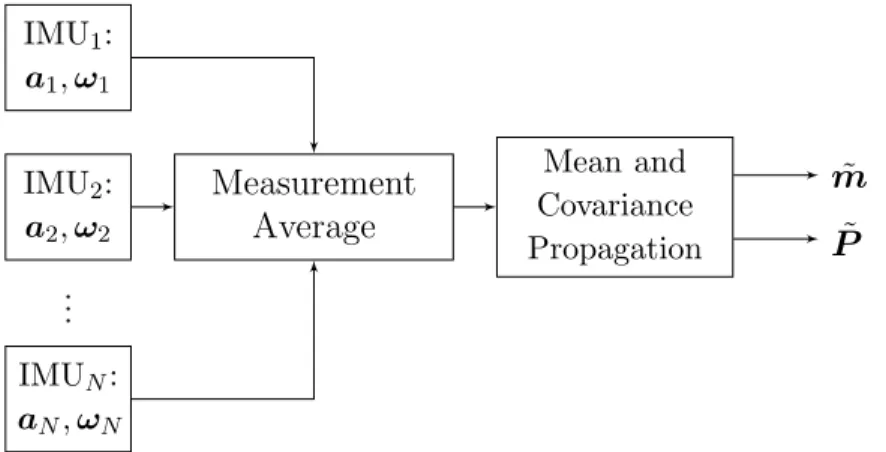
3.1. DIRECT AVERAGING
The direct averaging fusion approach takesN non-gravitational accelerations, transformed by the translational compensation discussed earlier, ai, and angular
ve-locities, ωi, from N IMUs and averages them together to determine a fused
non-gravitational acceleration, ˜a, and angular velocity, ˜ω. These fused data are then implemented in the dead-reckoning equations to produce a fused mean, ˜m, and co-variance, ˜P. For a set of L measurementsxi, the fused data ˜x is given by the direct
average ˜ x= 1 N N X i=1 xi, (3.1)
where xi = ai or xi = ωi. This method is the most simple fusion rule due to low
computational costs and can be easily implemented with analog circuitry. There are multiple averaging schemes applicable to IMU fusion such as averaging the state estimates and covariances after propagation, but for simplicity, the result of the fused raw measurements will be propagated to provide a fused navigation solution. This method of direct averaging is shown as a block diagram in Figure 3.1.
From Reference [1], the expectation in the improvement in bias stability and noise is on the order of √N, where N is the number of IMUs. In using a sensor
IMU1: a1,ω1 IMU2: a2,ω2 .. . IMUN: aN,ωN Measurement Average Mean and Covariance Propagation ˜ m ˜ P
Figure 3.1. IMU Data Fusion Computed by Directly Averaging the Measurements
network of redundant, homogeneous sensors, the actual improvement is expected to be slightly less than the √N factor because all noise sources cannot be assumed to be completely uncorrelated. To visualize this factor of improvement, sensor networks of N = 10, 100, and 1000 single degree of freedom accelerometers are simulated and averaged and are simply modeled in this case by injecting a bias an noise process into the true ai = 0 measurements. The fused measurement is plotted over that of
a single sensors in Figure 3.2. As expected it is seen that the noise is reduced by a
Single Accelerometer Data
Multiple Fused Accelerometer Data
0 2 4 6 8 10 −0.4 0 0.4 Time [s] 0 2 4 6 8 10 −0.4 0 0.4 Time [s] 0 2 4 6 8 10 −0.4 0 0.4 Time [s] ax,m [m/s 2 ]
significant factor as the number of sensors to be fused increases. This analysis of the direct averaging fusion rule exhibits simplicity; computationally and implementation wise. However, a more intelligent fusion rule is to be considered to examine fusion robustness.
3.2. COVARIANCE INTERSECTION
The covariance intersection (CI) rule is primarily known for fusing two Gaus-sian distributions by combining the means and covariances in order to produce con-sistent solutions. This approach can be described as a geometric representation of the Kalman filter because the form of the state estimate and covariance is identical to the standard Kalman filter, which can be found in Reference [3]. If the intersection of co-variance is known exactly, the cross coco-variance will always lie within the intersection of each of the respective covariances from Reference [3]. In order to examine the full form of CI, a general case is implemented in order to fuse N distributions together to produce a more accurate mean and covariance of the system. To derive the CI fusion rule, the geometric mean density (GMD) fusion rule proposed in Reference [4] is applied to N Gaussian distributions. The properties of the GMD fusion rule and more details of the GMD fusion are given in Reference [4]. The most general form of the GMD fusion rule for fusing N arbitrary probability density functions (pdfs) is
˜ p(x) = 1 η N Y i=1 pwi g (x;mi,Pi) (3.2)
where η is a normalization factor needed in order to have the distribution integrate to one and pg(x;m,P) represents a Gaussian distribution in x with mean m and
Raising a Gaussian distribution to the powerw, it follows that pwg (x;m,P) = |2πP|−1/2exp −1 2(x−m) T P−1(x−m) w =|2πP|−w/2expn−w 2 (x−m) T P−1(x−m)o
By defining ¯P , P/w, the Gaussian density raised to the power w may also be expressed as pwg (x;m,P) = |2πP|−w/2exp −1 2(x−m) T ¯ P−1(x−m) . (3.3)
The term within the exponential is of the form of the Gaussian distribution with a scaled covariance, but the normalizing factor does not account for the scaled co-variance. The normalizing factor should be |2πP¯|−1/2; therefore, multiplying and dividing the raised Gaussian in Eq. (3.3) by the proper normalizing constant gives
pwg (x;m,P) = kpg x;m,P¯
, (3.4)
where k = w−n/2|2πP|(1−w)/2. That is, a Gaussian distribution raised to the power w is a scaled Gaussian with an inflated covariance (provided that 0 ≤ w ≤ 1). Substituting the result of Eq. (3.4) into each term of the product in Eq. (3.2), it follows that the GMD fusion rule for Gaussian distributions is
˜ p(x) = 1 η N Y i=1 kipg x;mi,P¯i , (3.5) where ki =w −n/2 i |2πPi|(1−wi)/2 and ¯Pi =Pi/wi.
When the product is expanded out, the fused distribution of Eq. (3.5) becomes
˜ p(x) = ¯ k η pg x;m1,P¯1 pg x;m2,P¯2 pg x;m3,P¯3 · · ·pg x;mN,P¯N , (3.6)
where ¯k = QN
i=1ki. The product of two Gaussian distributions is a well known procedure [14], but this process becomes more complicated when considering N pdfs. Given two Gaussian pdfs pg(x;ma,Pa) and pg(x;mb,Pb), their product is [14]
pg(x;ma,Pa)pg(x;mb,Pb) = Γabpg(x;mc,Pc) , (3.7) where mc =Pc Pa−1ma+Pb−1mb (3.8a) Pc = Pa−1+Pb −1 (3.8b) Γab =|2π(Pa+Pb) −1/2 exp −1 2(ma−mb) T(P a+Pb)(ma−mb) . (3.8c)
Direct application of Eq. (3.7) to the product ofpg x;m1,P¯1
andpg x;m2,P¯2
in Eq. (3.6) gives the GMD as
˜ p(x) = ¯ k ηΓ12 pg x;m12,P¯12 pg x;m3,P¯3 · · ·pg x;mN,P¯N , (3.9)
where, from Eq. (3.5),
m12= ¯P12 P¯1−1m1+ ¯P2−1m2 (3.10a) ¯ P12= P¯1−1+ ¯P2 −1 (3.10b)
and similarly for Γ12. Now, apply Eq. (3.7) to the product of pg x;m12,P¯12
and pg x;m3,P¯3 in Eq. (3.9) to obtain ˜ p(x) = ¯ k ηΓ12Γ123 pg x;m123,P¯123 · · ·pg x;mN,P¯N , (3.11)
where, from Eqs. (3.8), it follows that m123 = ¯P123 P¯12−1m12+ ¯P3−1m3 ¯ P123 = P¯12−1+ ¯P3 −1 ,
and similarly for Γ123. From Eqs. (3.10), it follows thatm123and ¯P123 are equivalently expressed as m123 = ¯P123 P¯1−1m1+ ¯P2−1m2+ ¯P3−1m3 ¯ P123 = P¯1−1+ ¯P −1 2 + ¯P3 −1 .
It then follows that the GMD fusion rule for a set ofN Gaussian distributions is given by continuing to reduce products of pairs of Gaussian pdfs; therefore, by induction, the GMD fusion rule becomes
˜ p(x) = 1 η ¯ kΓ12Γ123· · ·Γ12···N pg(x; ˜m,P˜), (3.12) where ˜ m= ˜P N X i=1 ¯ Pi−1mi and P˜ = N X i=1 ¯ Pi−1 −1 .
Since the integral of ˜p(x) must evaluate to one and since the integral ofpg(x; ˜m,P˜)
is guaranteed to evaluate to one, it follows that η = ¯kΓ12Γ123· · ·Γ12···N.
Addition-ally, recall that ¯Pi = Pi/wi. Substituting for the normalizing factor and the scaled
covariances, the GMD fusion rule in Eq. (3.12) is given in its final form as
˜
where ˜ m= ˜P N X i=1 wiPi−1mi and P˜ = N X i=1 wiPi−1 −1 . (3.14)
Thus, the GMD fusion rule produces a Gaussian distribution when applied to a set of N input Gaussian distributions; in fact, Eq. (3.13) is exactly the CI method for fusing a set of N means and covariances.
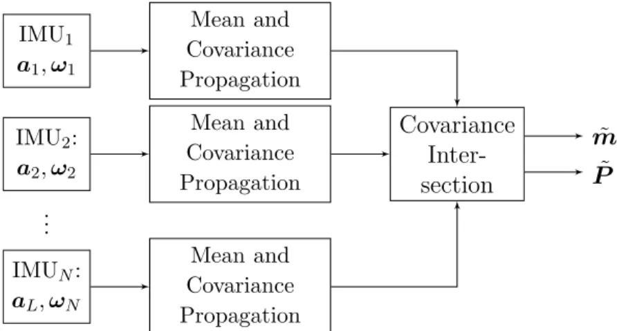
3.2.1. Implementation. The implementation using the CI fusion rule prop-agates the mean and covariance of each individual IMU and is followed by an applica-tion of CI at each time step to output a fused mean and covariance. This fusion rule is ideal for cheaper, fault-prone sensors in a distributed network by considering the weights correlated with CI. There are many different weighting techniques, although for brevity, only one will be examined. The process of the implementation of CI is outlined and shown in the block diagram in Figure 3.3.
IMU1 a1,ω1 IMU2: a2,ω2 .. . IMUN: aL,ωN Mean and Covariance Propagation Mean and Covariance Propagation Mean and Covariance Propagation Covariance Inter-section ˜ m ˜ P
Figure 3.3. IMU Data Fusion Computed by Covariance Intersection
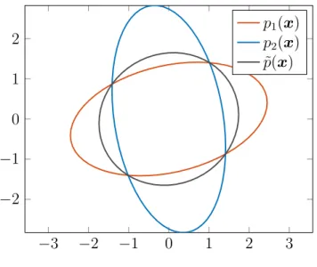
It is useful to visually see the effects of the CI fusion rule. Consider an ex-ample where two zero mean distributions, p1(x) and p2(x) respectively, with two
covariances and respective arbitrarily selected weights fused together using CI to pro-duce the fused distribution ˜p(x). The uncertainty ellipses based on their respective distributions are plotted with the fused uncertainty ellipse in Figure 3.4. It is seen
−3 −2 −1 0 1 2 3 −2 −1 0 1 2 p1(x) p2(x) ˜ p(x)
Figure 3.4. CI Fusion Rule
that the fused data produce a smaller uncertainty ellipse that geometrically is pro-jected and drawn through the intersections of the two distributions undergoing fusion. However, it is not practical to arbitrarily select weights for each covariance; therefore, a weighting scheme is needed to be shown.
3.2.2. Generalized Variance Weighting Selection. The covariance in-tersection algorithm depends on weighting low uncertainties larger than high uncer-tainties. One proposed method of weighting is taken from the generalized variance method, proposed by Wilks, found in Reference [15], as a scalar measure of overall multidimensional scatter. The generalized variance is the trace of the reciprocal of the information matrix, which in the fusion case is the trace of the covariance matrix tr{P}. With this knowledge, an algorithm for uncertainty weighting can be used to
intelligently weight the uncertain measurements. Noting that
L
X
i=1
wi = 1,
letP∗ be the sum of the determinants of the covariance matrices, such that
P∗ =
L
X
i=1 |Pi|.
The trace weights can then be appropriately given by
w∗i = tr{Pi}
P∗ .
However, this weighting scheme provides large weights for higher covariances which would allow for measurements with larger uncertainties to be trusted more than mea-surements with lower uncertainties. Noting that the above weight’s value is inversely proportional to the desired weight, the final expression for generalized variance weight selection given as wi = 1−w∗i PN `=1w ∗ ` . (3.15)
3.3. FAULT TOLERANT FUSION
IMU failures are typically very rare for most spacecraft due to the high fidelity nature of high-cost IMUs. In order to reduce the cost of using a single, high-cost, high-reliability tactical or strategic grade IMU, consider the case where multiple low-cost, commercial off-the-shelf (COTS) IMUs are used. In this case, the cost of a single high-cost, high-reliability IMU-based navigation system can be reduced by using a multiple low-cost IMU-based navigation system; however, this multiple IMU-based
system must be robust to faults in the IMUs as the lower-cost COTS IMUs have a non-negligible possibility of failure as compared to the single high-cost IMU.
Two fault tolerant frameworks are considered for this multiple IMU-based navigation system: direct averaging of the measured acceleration and angular velocity provided by each IMU and fusing the dead-reckoned state of each IMU using the CI method. The direct averaging method is expected to provide an estimate of the vehicle state with a lower uncertainty than is obtained by fusing the individual dead-reckoned navigation solutions using the covariance intersection method. When fusing the individual dead-reckoned navigation solutions using CI, the weights used for CI are selected as a function of the uncertainty in each dead-reckoned solution; thus, this fusion rule is predicted to be more robust than the direct averaging fusion rule. The uncertainty in the dead-reckoned solution corresponding to a failed sensor will become very large, which means that its weight will tend to zero, thereby effectively removing its influence on the fused navigation solution.
In order to take advantage of both the lower uncertainty obtained when direct averaging the measured accelerations and angular velocities and the robustness of fusing the individual navigation solutions using the CI method, a system is proposed that runs both algorithms in parallel and uses the dead-reckoned solution correspond-ing to the direct averagcorrespond-ing method in the presence of no sensor failures. As a safe mode, the algorithm will switch to using the fused navigation solution given by the CI method in the case of sensor failure(s). This algorithm is summarized by Algo-rithm 1 in Appendix B. In order for the uncertainty of the individual dead-reckoned navigation solutions, P1,...,N, to propagate accurately, it is assumed that real-time
values for the error parameters of each IMU are available from some type of real-time sensor calibration. This will cause Pi to grow more quickly when IMUi fails and
produces more corrupted data than normal. If these data are blindly averaged, as is proposed in the direct averaging method, after a fault occurs in the system, then the
navigation solution corresponding to this method can no longer accurately represent the covariance. In the case where the weights used in CI fusion can down-weight failing sensors, the averaging fusion rule cannot be considered robust. As of now the covariances being fused are modeled as the true uncertainty of the system which is not the case in performing linear covariance. With this assumed knowledge of sensor and covariance degradation, CI is expected to down-weight dead-reckoned solutions with higher uncertainties acting as a pseudo fault detection method.
3.4. FUSION EXAMPLE
To demonstrate the performance of the proposed direct averaging and covari-ance intersection fusion methods, a simulation is performed in which the navigation solution fused from six low-cost IMUs is compared against the navigation solution ob-tained using a single tactical grade IMU. The true non-gravitational acceleration and angular velocities of the simulated IMUs are simulated for a spacecraft in LEO using AGI STK1 with a primary spin about the body z-axis. The true accelerations and angular velocities are corrupted according to the error model given in Eqs. (2.1). The error parameters for these models are based off of the Microstrain 3DM-GX3-152 and the Epson M-G362PDC13 IMUs and are summarized in Appendix A. Three of each IMU are assumed to be on the spacecraft, which is considered to be a 1.0×1.0×1.0 meter cube. The locations of each of the six IMUs as well as the CM of the spacecraft are shown in Table 3.1.
In order to compare the direct averaging and CI fusion rules, consider the case where one of the Microstrain 3DM-GX3-15 IMUs fails at t = 100 s, an arbi-trarily chosen time, and begins to provide more corrupted data. Because the noise characteristics of this more corrupted data are assumed known, the uncertainty in
1http://www.agi.com/products/stk/
2http://www.microstrain.com/inertial/3dm-gx3-35
Table 3.1. Spacecraft IMU Configuration IMU Position Vector [m]
CG IMU2 IMU6 IMU1 IMU4 IMU3 IMU5 IMU1: M-G362PDC1 d1 = 0.0 0.0 0.5 IMU2: M-G362PDC1 d2 = 0.0 0.5 0.0 IMU3: M-G362PDC1 d3 = 0.5 0.0 0.5 IMU4: 3DM-GX3-15 d4 = 0.0 −0.5 0.0 IMU5: 3DM-GX3-15 d5 = −0.5 0.0 0.0 IMU6: 3DM-GX3-15 d5 = 0.0 0.0 −0.5
the navigation solution associated with this IMU begins to grow very quickly. For brevity, only the position and attitude uncertainties are presented because the po-sition and velocity uncertainties follow the same general trends and uncertainty is the most effective way to evaluate the fusion rules. The legend used for presenting the results is shown in Table 3.2. To provide information on the trend of
uncer-Table 3.2. Fusion Example Legend Single 3DM-GX3-15 IMU Failure Systron Donner: SDI-500 (Not Fused) Epson: M-G362PDC1
Micro Strain: 3DM-GX3-15
Covariance Intersection Fusion Rule Direct Averaging Fusion Rule
tainty growth, the position and attitude root-sum-square (RSS) are shown in Figure 3.5. The failure of the single Microstrain 3DM-GX3-15 IMU at t = 100 s causes an instantaneous change in how the uncertainty of the single IMU dead-reckoning nav-igation solution evolves. In the case of the position RSS, because the failure causes changes to the IMU acceleration, the effects are less immediate due to the necessity
0 20 40 60 80 100 120 140 160 180 200 220 240 260 280 300 0 0.1 0.2 0 20 40 60 80 100 120 140 160 180 200 220 240 260 280 300 0 200 400 600 800
Figure 3.5. Position [m] and Attitude [deg] RSS Error
of doubly integrating the acceleration. In terms of the fusion rules, however, the position RSS demonstrates the quickest switch between the direct averaging fusion rule and the CI fusion rule. At approximately t = 125 s, the CI fusion rule begins to outperform the direct averaging fusion rule in position uncertainty. This reversal occurs only at approximately t= 180 s in the attitude uncertainty. In order to show the uncertainty in the position with less cluttered plots, a series of two dimensional uncertainty contour plots in the x−y plane are shown at t = 50, 200, and 300 s in Figure 3.6. The first time step shows the position uncertainty before any IMU failure, which illustrates that the direct averaging fusion rule provides a more confident navi-gation solution in the presence of no IMU failures. The next two time steps show the position uncertainty after the IMU failure, demonstrating that the CI fusion rule is preferred in the case of an IMU failure. While the direct averaging fusion rule clearly follows along with the failed IMU, the CI fusion rule downweights the failed IMU and is seen to be consistent with the remaining, nominally operating IMUs. However, the CI fusion rule has no knowledge of a sensor failure so a comparison of the two fusion
−2,000 0 2,000 −2,000 −1,000 0 1,000 2,000 −500 0 500 −600 −400 −200 0 200 400 600 −10 0 10 −10 0 10
Figure 3.6. x−y Uncertainty Contours [m] at 50, 200, 300 [s], Respectively
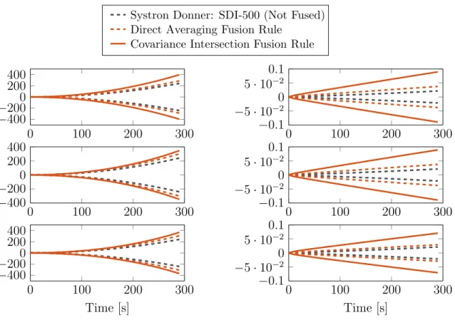
rules’ true covariance outputs are shown for position and attitude in Figure 3.7. It can be determined that the true uncertainty of data averaging system undergoing no sensor failures can be characterized much closer to that of a tactical grade IMU. The CI fusion rule cannot obtain a covariance navigation solution lower than the lowest individual sensor which promotes direct averaging over CI.
3.5. FUSION METHODOLOGY SUMMARY AND CONCLUSION
In order to provide a lower-cost inertial measurement unit (IMU)-based navi-gation system as opposed to one that uses a typical high-cost, high-reliability tactical or strategic grade IMU, a fault-tolerant method was proposed that uses multiple low-cost IMUs and fuses their data together via a direct averaging method or fuses their individual navigation solutions together via the covariance intersection (CI) fusion rule. It is demonstrated that the direct averaging fusion rule tends to outperform the CI fusion rule during nominal operations where no hardware failures are present. On the other hand, the CI fusion rule is shown to outperform the direct averaging fusion rule when an IMU fails due to the ability of the CI fusion rule to selectively down-weight the navigation solution obtained from the failed IMU. The proposed algorithm
Systron Donner: SDI-500 (Not Fused) Direct Averaging Fusion Rule
Covariance Intersection Fusion Rule
0 100 200 300 −400 −2000 200 400 Time [s] 0 100 200 300 −400 −200 0 200 400 0 100 200 300 −400 −2000 200 400
(a) Fused Position Uncertainty [m]
0 100 200 300 −0.1 −5·10−2 0 5·10−2 0.1 Time [s] 0 100 200 300 −0.1 −5·10−2 0 5·10−2 0.1 0 100 200 300 −0.1 −5·10−2 0 5·10−2 0.1
(b) Fused Attitude Uncertainty [deg] Figure 3.7. Fusion Rule Uncertainty Comparison
uses the navigation solution propagated using the direct averaged data when there are no IMU faults because it provides a more confident solution. In the case of an IMU failure, the algorithm will recognize the failure, and the navigation solution from the covariance intersection method will be used. However, the covariance propagation is a function of sensor errors given from data sheet specifications. The uncertainties undergoing failures were realized by adding in the sensor failure parameters into the IMU model forcing knowledge of the failure. If the covariance propagation could au-tonomously detect changes in sensor parameters, then CI would be the robust, fault tolerant fusion method. However, this error realization is not likely or realistic. It was seen in the results that a simple averaging fusion method produces a more accu-rate navigation solution than that of CI concluding that direct averaging is the best
option for IMU data fusion. Therefore, data averaging has no knowledge of faulty data, a fault detection architecture must be examined and implemented to provide a true fault tolerant multi-sensor network on-board a spacecraft.
4. FAULT DETECTION
To reiterate the conclusions of the comparison of direct averaging and CI, direct averaging out performs CI in the case of no faults. It was also seen that if a sensor failure is present, CI has the robust ability to recognize the fault if weighted correctly. Unfortunately, the proposed weighting solution is a function of covariance which is computed from sensor data sheet statistics and specifications. This leaves both fusion methods with the need for a robust, fault detection scheme, and due to the higher estimate direct averaging has to offer, the proposed fusion method in the considerations of fault detection is that of direct averaging. Principal Component Analysis (PCA) is the initial proposed fault detection method. However, an example is shown concluding in the need of a more desirable, modified version of PCA that better fits the dynamic nature of IMUs.
4.1. PRINCIPAL COMPONENT ANALYSIS
Principal Component Analysis (PCA) has many applications, such as dimen-sionality reduction, feature extraction and data visualization. While dimendimen-sionality reduction does not have much application to detecting faults in IMU data, feature extraction and data visualization play an important role in recognizing faults in an IMU sensor network. From Bishop [16], there are two commonly used definitions of PCA consisting of a maximum variance formulation and a minimum-error formula-tion. The maximum variance formulation orthogonally projects data onto a linear space with lower dimension such that the variance of the transformed data is maxi-mized. This linear space is known as the principle subspace or the feature plane. The minimum-error formulation linearly projects the data while minimizing the average projection cost. Each method is equivalent, and the studied PCA definition will be that of the maximum variance formulation. In the case where there is no dynamical
movement, consider a multiple IMU sensor network with N number of IMUs. Fol-lowing procedures from Lee [8] and Bishop [16], the first step is to fuse the data by directly averaging the measurements to get xavg, governed by
xavg = 1 N N X i=1 ˆ xi, (4.1)
where ˆxi ∈ Rm is the measured outputs from each IMU i.e. ai or ωi. A data set
is then constructed to produce zero mean data, mp,i, by subtracting the averaged
output from each measurement given as
mp,i = ˆxi−xavg, (4.2)
The next step is to compute the measurement covariance matrix. By definition the covariance is given by P = E n (x−E[x]) (x−E[x])T o ,
which can be notationally written for a multi-sensor system as
P = 1 N N X i=1 ( ˆxi−xavg) ( ˆxi−xavg)T (4.3) = 1 N N X i=1 mp,imTp,i, ∈R m×m . (4.4)
This covariance can be written in terms of its eigenvectors and eigenvalues, such that
P =VΓVT, V =
v1 v2 · · · vm
(4.5)
where V ∈ Rm×m is the eigenvector matrix of P composed of m unit eigenvectors vi, and Γ ∈Rm×m is the diagonal eigenvalue matrix of P. This is found by solving
the characteristic equation
(P −λiIm×m)vi =0, (4.6)
whereλi and vi denote the ith eigenvalue and eigenvector respectively. The
eigenvec-tors and eigenvalues are introduced as a representation of the variance in the data due to their orthogonality, which exposes patterns in the data. This pattern can be thought of as a relationship of the data sets that are related along a best-fit line. The most significant relationship between the data sets is known as the principle compo-nent and can be represented by the eigenvector with the largest eigenvalue. Once all eigenvector and eigenvalue pairs are found, it is important to list them from largest to smallest which will give an ordering of significance to the components known as a feature vector matrix Φ. Components of lesser significance can then be ignored; however, some information will be lost, but this can be considered negligible for most cases. The feature matrix can be written in terms of the most significant eigenvectors to lowest written as Φ= φ∗1 φ∗2 · · · φ∗s ,
where the ∗ superscript represents the eigenvectors in order of most significant to least, and the subscript s denotes the number of selected dimensions used where
s ≤ m. The feature vector constructed is then used to transform the original data into a new data set that shows the sensor’s data patterns; the transformed data is
y=ΦT ˆ x1 xˆ1 · · · xˆN T , (4.7)
where y is the transformed data set that correlates the original data with a sensor pattern. While this case is only useful for a sensor with no movement, PCA can
be used for sensor calibration and fault detection when the system is at rest. This also lays the foundation for MPCA, which will provide fault tolerant algorithms for dynamical systems.
4.2. FAULT DETECTION EXAMPLE
A motivating example is provided to compare PCA for a static and dynamic accelerometer. Consider six (L= 6) 3-axis (m = 3) accelerometer systems assuming each accelerometer is at the center of mass. Throughout the example two selected dimensions for the feature matrix (s = 2) are used. The static measurements are simulated by corrupting a true acceleration ofas=0and the dynamic measurements
are simulated from the equations of motion given by ad =
sin2(θ) cos(θ) 0.0T whereθ=t∆t[rad]. The example is carried out with ∆t= 0.01 [s], with a simulation time of 10 seconds, tf = 10 [s]. At 5 seconds into the simulation, accelerometer three
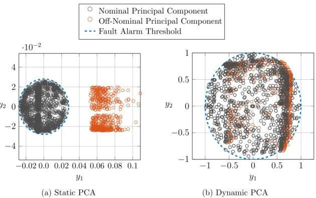
undergoes an increase in bias and noise, simulating a sensor fault. This example is used to prove and visualize the need for a modified version of PCA for dynamic systems. The measurements are then transformed using principal components based on Eq. (4.7). Figure 4.1 shows the effects and behavior of PCA applied on the static and dynamic systems.
Note thaty1 is the dominant information holder in the feature plane due to the feature vector matrix Φ giving preference to the most significant eigenvector. After a failure y1 is dominated by the fault allows for the fault to expose itself while y2 is dominated by the patterns of sensor noise. It is seen that in the static case, PCA is able to easily identify threshold outliers enabling a fault alarm to disregard the outlying measurements. The threshold value is selected based on the interpretation on what is and is not a failure. A fault alarm is determined by pulling a fault identification signal high to alert the system of a failure with a corresponding sensor ID (i = 3) in this case. This method is discussed in depth in the simulation results
Nominal Principal Component Off-Nominal Principal Component Fault Alarm Threshold
−0.02 0.0 0.02 0.04 0.06 0.08 0.1 −4 −2 0 2 4 ·10−2 y1 y2
(a) Static PCA
−1 −0.5 0 0.5 1 −1 −0.5 0 0.5 1 y1 y2 (b) Dynamic PCA
Figure 4.1. Effects of PCA Undergoing Single Sensor Failure for Static and Dynamic Systems
section. However, in the dynamic case, the principal components containing fault information cannot be distinguished from the nominal principal components proving a need to remove dynamic effects from the feature plane. This is the goal when modifying the principal component analysis method.
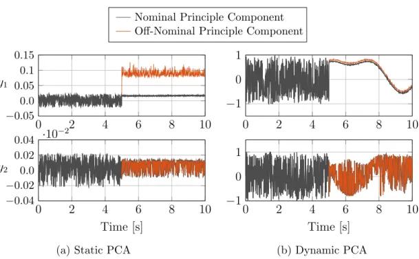
In Figure 4.1, it is seen that principal components tend to shrink in the first principal component direction. When plotted in two dimensions (y1 vs. y2), this decrease in the first principal component is not easily seen; therefore, each principal component is plotted separately versus time for the static case and the dynamic case and is shown in Figure 4.2.
While the clustered data points in the two dimensional plots become apparent from the one dimensional plots, it is desired to seek an explanation for the drastic decrease in the feature plane along the first principal component. The static case is examined in order to conclude a reasoning for this phenomena. It is known that the
Nominal Principle Component Off-Nominal Principle Component
0 2 4 6 8 10 −0.04 −0.02 0.0 0.02 0.04 ·10 −2 Time [s] y2 0 2 4 6 8 10 −0.05 0.0 0.05 0.1 0.15 y1
(a) Static PCA
0 2 4 6 8 10 −1 0 1 Time [s] 0 2 4 6 8 10 −1 0 1 (b) Dynamic PCA
Figure 4.2. First and Second Principal Components versus Time for a Static and Dynamic System Undergoing a Single Sensor Failure
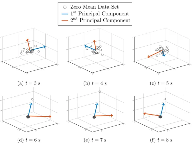
direction of the eigenvectors, used as the first and second principal components, are orthogonal and geometrically point along the best-fit lines through data along the first and second principal directions. The eigenvector pairs are plotted over a point cloud of zero-mean data in three dimensions for twenty sensors instead of the six sensors priorly used to emphasize the illustration. In the current discussion of fault detection, faulty data is denoted as off-nominal components, and the functional data is denoted as nominal components. These illustrations are plotted at three epochs prior-and post-failure and are shown in Figure 4.3.
From the PCA derivation, it is known that the feature plane is a function of the principal eigenvectors and the data set. Figures 4.3a-4.3c shows direction of the principal components pointing along the best fit line through the data. It is seen that both eigenvectors are pointing in drastically different directions at each epoch that accounts for the “noisy” feature plane patterns before the failure. Examining the
Zero Mean Data Set 1st Principal Component 2nd Principal Component
(a)t= 3 s (b) t= 4 s (c)t= 5 s
(d) t= 6 s (e) t= 7 s (f) t= 8 s
Figure 4.3. First and Second Principal Components Plotted Over 3-Dimensional Zero-Mean Data Set Before and After Failure
failure case in Figures 4.3d-4.3f, it is seen that the best fit line along the 1st principal component is along the direction of the faulty sensor data. The 1st principal compo-nent’s variation remains relatively constant after the fault in order to geometrically satisfy the best fit line along the fault.
4.3. MODIFIED PRINCIPAL COMPONENT ANALYSIS
Recall that PCA can only be used for a non-moving sensor due to the fault-like data patterns caused by sensor motion. Hence, the Modified Principle Component Analysis (MPCA) is introduced to allow for fault detection in a dynamic system. This modified method uses a training data set ˆxT, which is the measured IMU outputs from
[8], the parity space concept is implemented, which helps remove the negative effects caused by sensor movement.
A matrixΘis required in order to formulate the parity space, which is defined as the column space of Θand is defined by the following conditions: Θis a positive definite trapezoidal matrix that satisfies the conditions [8]
ΘH =0, ΘΘT =I ∈Rn−ζ×n−ζ, and Θ= θ1 θ2 · · · θn−ζ T = θc,1 θc,2 · · · θc,n,
where H is the sensor orientation matrix that defines the physical sensor placement and rotation for the distributed system of IMUs,nis the number of sensors used, and
ζ is the rank of H. The first step in computing theΘmatrix is to find the null space of H, which will be denoted as N; that is,
N = null (H).
Then, to ensure that the needed conditions are satisfied, a QR factorization method [17] is applied to N and the resulting R matrix in the factorization is the Θmatrix. Using this method,N can be decomposed into two matricesQandR. TheRmatrix formulated from this null space meets all of the conditions for Θ and is formally defined as
where Q is an m×m unitary matrix and R (or Θ) is an upper triangular matrix; hence, Θis trapezoidal in this case.
As stated before a training vector is used to remove the dynamic effects in the feature plane. A training parity matrix is found by multiplying a subset of the columns ofΘ and the training vector as
pT = θ1 θ2 · · · θm ˆ xT.
This training parity matrix is now a function of sensor movement based on the training vector. The feature vector used to transform the data into the feature plane in the MPCA formulation YT can then be calculated by finding the null space of pT to
effectively create a matrix that negates dynamic effects and is given as
YT = null(pT).
A parity matrix, which transforms all measurements into the same orientation space, is computed as p=Θ ˆ x1 xˆ1 · · · xˆN T .
The columns of Θ are defined as the projections of the direction of measurements onto the parity space. The parity matrix and dynamic null space matrix are used to create a sub-transformed data set, y∗, which is not a function of sensor movement, and is given as
![Figure 3.5. Position [m] and Attitude [deg] RSS Error](https://thumb-us.123doks.com/thumbv2/123dok_us/1455724.2694773/44.918.220.755.109.457/figure-position-m-attitude-deg-rss-error.webp)
![Figure 3.6. x − y Uncertainty Contours [m] at 50, 200, 300 [s], Respectively](https://thumb-us.123doks.com/thumbv2/123dok_us/1455724.2694773/45.918.212.776.103.365/figure-uncertainty-contours-at-respectively.webp)