Low-rank matrix factorization in multiple kernel
learning
A dissertation presented byMartin Stražar
toThe Faculty of Computer and Information Science in partial fulfilment of the requirements for the degree of
Doctor of Philosophy in the subject of
Computer and Information Science
APPROVAL
I hereby declare that this submission is my own work and that, to the best of my knowledge and belief, it contains no material previously published or written by another person nor material which to a substantial extent has been accepted for the award of any other degree or diploma of the university or other institute of higher learning, except where
due acknowledgement has been made in the text.
— Martin Stražar, September
The submission has been approved by dr. Tomaž Curk
Assistant Professor of Computer and Information Science advisor
University of Ljubljana, Faculty of Computer and Information Science dr. Matej Kristan
Associate Professor of Computer and Information Science examiner
University of Ljubljana, Faculty of Computer and Information Science dr. Bor Plestenjak
Professor of Mathematics examiner
University of Ljubljana, Faculty of Mathematics and Physics dr. Dino Sejdinović
Associate Professor in Statistics examiner
PREVIOUS PUBLICATION
I hereby declare that the research reported herein was previously published/submitted for publication in peer reviewed journals or publicly presented at the following occa-sions:
[] M. Stražar, J. Ule, B. Zupan, M. Žitnik, and T. Curk. Orthogonal matrix factorization enables integrative analysis of multiple RNA binding proteins. In Jonathan Wren, editors, volume . ofBioinformatics, pages –, Oxford, . Oxford University Press.
I certify that I have obtained a written permission from the copyright owner(s) to include the above published material(s) in my thesis. I certify that the above material describes work completed during my registration as graduate student at the University of Ljubljana.
ABSTRACT
Universityof Ljubljana
Facultyof Computer and Information Science
Martin Stražar
Low-rank matrix factorization in multiple kernel learning
The increased rate of data collection, storage, and availability results in a correspond-ing interest for data analyses and predictive models based on simultaneous inclusion of multiple data sources. This tendency is ubiquitous in practical applications of ma-chine learning, including recommender systems, social network analysis, finance and computational biology. The heterogeneity and size of the typical datasets calls for si-multaneous dimensionality reduction and inference from multiple data sources in a single model. Matrix factorization and multiple kernel learning models are two gen-eral approaches that satisfy this goal. This work focuses on two specific goals, namely i) finding interpretable, non-overlapping (orthogonal) data representations through matrix factorization and ii) regression with multiple kernels through the low-rank ap-proximation of the corresponding kernel matrices, providing non-linear outputs and interpretation of kernel selection.
The motivation for the models and algorithms designed in this work stems from RNA biology and the rich complexity of protein-RNA interactions. Although the regulation of RNA fate happens at many levels - bringing in various possible data views - we show how different questions can be answered directly through constraints in the model design. We have developed an integrative orthogonality nonnegative matrix factorization (iONMF) to integrate multiple data sources and discover non-overlapping, class-specific RNA binding patterns of varying strengths. We show that the integration of multiple data sources improves the predictive accuracy of retrieval of RNA binding sites and report on a number of inferred protein-specific patterns, consistent with experimentally determined properties.
A principled way to extend the linear models to non-linear settings are kernel meth-ods. Multiple kernel learning enables modelling with different data views, but are limited by the𝑂(𝑛)computation and storage complexity of the kernel matrix.
ii Abstract M. Stražar siderable savings in time and memory can be expected if kernel approximation and multiple kernel learning are performed simultaneously. We present the Mklaren al-gorithm, which achieves this goal via Incomplete Cholesky Decomposition, where the selection of basis functions is based on Least-angle regression, resulting in linear complexity both in the number of data points and kernels. Considerable savings in approximation rank are observed when compared to general kernel matrix decompo-sitions and comparable to methods specialized to particular kernel function families. The principal advantages of Mklaren are independence of kernel function form, robust inducing point selection and the ability to use different kernels in different regions of both continuous and discrete input spaces, such as numeric vector spaces, strings or trees, providing a platform for bioinformatics.
In summary, we design novel models and algorithms based on matrix factorization and kernel learning, combining regression, insights into the domain of interest by identifying relevant patterns, kernels and inducing points, while scaling to millions of data points and data views.
Key words:Machine learning, bioinformatics, matrix factorization, kernel methods, multiple kernel learning, linear regression, protein-RNA interactions.
POVZETEK
Univerzav Ljubljani
Fakultetaza računalništvo in informatiko
Martin Stražar
Faktorizacija matrik nizkega ranga pri učenju z večjedrnimi metodami
V času pospešenega zbiranja, organiziranja in dostopnosti podatkov se pojavlja potreba po razvoju napovednih modelov na osnovi hkratnega učenja iz več podatkovnih virov. Konkretni primeri uporabe obsegajo področja strojnega učenja, priporočilnih siste-mov, socialnih omrežij, financ in računske biologije. Heterogenost in velikost tipičnih podatkovnih zbirk vodi razvoj postopkov za hkratno zmanjšanje velikosti (zgoščevanje) in sklepanje iz več virov podatkov v skupnem modelu. Matrična faktorizacija in jedrne metode (ang.kernel methods) sta dve splošni orodji, ki omogočata dosego navedenega cilja. Pričujoče delo se osredotoča na naslednja specifična cilja: i) iskanje interpretabil-nih, neprekrivajočih predstavitev vzorcev v podatkih s pomočjo ortogonalne matrične faktorizacije in ii) nadzorovano hkratno faktorizacijo več jedrnih matrik, ki omogoča modeliranje nelinearnih odzivov in interpretacijo pomembnosti različnih podatkovnih virov.
Motivacija za razvoj modelov in algoritmov v pričujočem delu izhaja iz RNA bio-logije in bogate kompleksnosti interakcij med proteini in RNA molekulami v celici. Čeprav se regulacija RNA dogaja na več različnih nivojih — kar vodi v več podatkov-nih virov/pogledov — lahko veliko lastnosti regulacije odkrijemo s pomočjo omejitev v fazi modeliranja. V delu predstavimo postopek hkratne matrične faktorizacije z ome-jitvijo, da se posamezni vzorci v podatkih ne prekrivajo med seboj — so neodvisni oz. ortogonalni. V praksi to pomeni, da lahko odkrijemo različne, neprekrivajoče nači-ne regulacije RNA s strani različnih proteinov. Z vzključitvijo več podatkovnih virov izboljšamo napovedno točnost pri napovedovanju potencialnih vezavnih mest posa-meznega RNA-vezavnega proteina. Vzorci, odkriti iz podatkov so primerljivi z ekspe-rimentalno določenimi lastnostmi proteinov in obsegajo kratka zaporedja nukleotidov na RNA, kooperativno vezavo z drugimi proteini, RNA strukturnimi lastnostmi ter funkcijsko anotacijo.
iv Povzetek M. Stražar Klasične metode matrične faktorizacije tipično temeljijo na linearnih modelih po-datkov. Jedrne metode so eden od načinov za razširitev modelov matrične faktorizacije za modeliranje nelinearnih odzivov. Učenje z več jedri (ang.Multiple kernel learning) omogoča učenje iz več podatkovnih virov, a je omejeno s kvadratno računsko zahtev-nostjo v odvisnosti od števila primerov v podatkih. To omejitev odpravimo z ustrezni-mi približki pri izračunu jedrnih matrik (ang. kernel matrix). V ta namen izboljšamo obstoječe metode na način, da hkrati izračunamo aproksimacijo jedrnih matrik ter nji-hovo linearno kombinacijo, ki modelira podan tarčni odziv. To dosežemo z metodo Mklaren (ang.Multiple kernel learning based on Least-angle regression), ki je sestavljena iz Nepopolnega razcepa Choleskega in Regresije najmanjših kotov (ang. Least-angle regression). Načrt algoritma vodi v linearno časovno in prostorsko odvisnost tako gle-de na število primerov v podatkih kot tudi glegle-de na število jedrnih funkcij. Osnovne prednosti postopka so poleg računske odvisnosti tudi splošnost oz. neodvisnost od uporabljenih jedrnih funkcij. Tako lahko uporabimo različne, splošne jedrne funkcije za modeliranje različnih delov prostora vhodnih podatkov, ki so lahko zvezni ali dis-kretni, npr. vektorski prostori, prostori nizov znakov in drugih podatkovnih struktur, kar je prikladno za uporabo v bioinformatiki.
V delu tako razvijemo algoritme na osnovi hkratne matrične faktorizacije in jedr-nih metod, obravnavnamo modele linearne in nelinearne regresije ter interpretacije podatkovne domene - odkrijemo pomembna jedra in primere podatkov, pri čemer je metode mogoče poganjati na milijonih podatkovnih primerov in virov.
Ključne besede:Strojno učenje, bioinformatika, matrična faktorizacije, jerdne metode, učenje z več jedrnimi funkcijami, linearna regresija, interakcije proteini-RNA.
ACKNOWLEDGEMENTS
This book is a small piece of puzzle in the vast scientific world. On the other hand, it constitutes a major part of what I have learned in the last couple of years, which has been possible with the help of numerous persons, to whom I express my sincere gratitude.
My thesis advisor dr. Tomaž Curk, University of Ljubljana, and dr. Jernej Ule, The Crick Institute, London, for introducing me to computational RNA biology, and providing critical feedback on a regular basis. To be part of a dynamic, international team and a fast-paced environment is the best a graduate student can wish for.
The head of Biolab at University of Ljubljana, dr. Blaž Zupan, for sharing impor-tant lessons in science and beyond, and being a great example of perseverance and resisting instances of higher power.
The coworkers at Biolab, fellow teachers and other staff members at the Faculty for a pleasant working and social environment.
To Tina and my family — Olga, Božo and Eva — for supporting me, which I often did not make any easier.
— Martin Stražar, Ljubljana, September .
CONTENTS
Abstract i
Povzetek iii
Acknowledgements v
Introduction
. Data integration by matrix factorization . . .
. Low-rank approximation of multiple kernel matrices . . .
. Summary of the scientific contributions . . .
. Availability . . .
. Overview of thesis structure . . .
Low-rank matrix approximation
. Notions of error . . .
. Non-negative matrix factorization . . .
. Constrained matrix factorization . . .
. Simultaneous matrix factorization . . .
Integrative orthogonal nonnegative matrix factorization
. The iONMF model and algorithms . . .
. Derivation of the iONMF optimization algorithm . . .
. The prediction function . . .
. Discovering relevant modules and features . . .
viii Contents M. Stražar
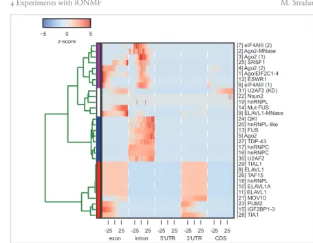
Experiments with iONMF
. Sampling of genomic positions . . .
. Data matrices . . .
. Analysis overview . . .
. Predictive performance . . .
. Effect of orthogonality . . .
. Overlap between modules . . .
. Estimated importance of data sources . . .
. Identified factors associated with RBP binding . . .
.. iONMF identifies biologically relevant binding patterns . .
.. Orthogonality constraints demultiplex binding patterns . . .
. Summary on biological results . . .
. Summary on orthogonal matrix factorization . . .
Kernel methods
. Kernel functions . . .
. Output function spaces . . .
. Multiple kernel learning . . .
.. Making new kernels from old . . .
.. Multiple kernel learning algorithms . . .
. Gaussian processes . . .
. Kernel matrix approximations . . .
. Kernel-specific approximations . . .
Approximate multiple kernel learning
. Initial definitions and overview . . .
. Simultaneous Incomplete Cholesky decompositions . . .
. Pivot selection based on Least-angle regression . . .
. Look-ahead decompositions . . .
. The Mklaren algorithm . . .
. Out-of-sample prediction . . .
. Computing dual coefficients . . .
. 𝐿norm regularization . . .
Low-rank kernel approximation ix
. A function space view . . .
Experiments with Mklaren
. A note on compared methods . . .
. Robust selection of inducing points . . .
.. Inducing points location distributions . . .
.. Matching pursuit versus Least-angle regression . . .
. Time series . . .
. String kernels . . .
.. Experiments on synthetic data . . .
.. Predicting RNA-binding protein binding affinities . . .
. Compactness of approximations . . .
. Comparison of MKL methods on rank-one kernels . . .
. Empirical execution times . . .
. Summary of the results on approximate MKL . . .
Conclusion
A A brief introduction to RNA biology
B Details on derivations and algorithms
B. Low-rank matrix approximation . . .
B.. Notions of error . . .
B.. Principal component analysis . . .
B. Linear regression . . .
B.. The relation between dual and primal regression weights . .
B.. Least-angle regression . . .
B. Kernel methods . . .
B.. Inner product spaces . . .
B.. A simple example of (kernel) linear regression . . .
B.. Kernel-specific approximations . . .
B.. Translation-invariant kernels and explicit feature maps . . .
x Contents M. Stražar
C Supplementary Information on iONMF
C. Detailed information on analyzed RBP experiments . . .
C. Details on models inferred from subsets of data sources . . .
C. Importance of different data sources . . .
C.. Prediction accuracy of data source subsets . . .
C.. Mutual information within individual data sources . . .
C.. Clustering of RBPs based on individual data sources . . . .
D Razširjeni povzetek
Introduction
Introduction M. Stražar Data integration in machine learning refers to the exploitation of multiple data sources to improve model interpretability and performance. With the increased rate of data collection, storage, and availability, there exist a corresponding interest for data anal-yses and predictive models based on simultaneous inclusion of multiple data sources. This tendency is ubiquitous in practical applications of machine learning; in recom-mender systems, side information collected on the customers along with their prefer-ences and purchase history improves future recommendations []; similarly, social network analysis and prediction is improved by modelling explicit dependencies be-tween users []; bioinformatics and precision medicine are often based on modelling a biological system behavior spanning multiple, inter-dependent regulatory levels, for example: gene expression, metabolic pathways, or macromolecule interactions [,]. The heterogeneity and sheer size of the data sets in these domains must be addressed by tailored models and algorithms, providing scalable inference and interpretable de-cisions. The scalability problem can be solved with an appropriate dimensionality reduction scheme that results in model or data approximation. In a technical sense, the heterogeneity of data sets might present itself as features-of-features [,], fixed relations between multiple object types [], class labels [], or multiple possible ways to measure object similarity, e.g. in kernel-based learning []. Hence, the two seem-ingly limiting properties within mentioned domains should be encoded within a single model.
Colloquially, the termdata integrationordata fusionhas first arisen as the problem of combining different sensory information coming from one or more sensors [,]. The methods forming this field can be broadly split into three major categories [];
early integrationcomprises problems of merging the input data into a single data struc-ture to be used with standard machine learning models. Inlate integration, an inde-pendent model is inferred for each data source, and the corresponding multiple predic-tions are combined at a later stage by a form of averaging. Both of the aforementioned strategies disregard the modular structure of the data. Finally, inintermediate integra-tion, a single model is inferred by selecting information from multiple data sources, exploiting the information of the implicit structure assumed by multiple data sources. This work focuses on two specific goals within intermediate data integration model, with the goal of finding:
Low-rank kernel approximation
-orthogonal matrix factorization, and
. complementary information within multiple similarity measures in order to model the target response -multiple kernel regression.
The proposed algorithms are rigorously evaluated using general benchmark, as well as domain specific data sets. Additionally, we provide extensive experiments on re-alistic data sets in the bioinformatics domain. The motivations, challenges and brief descriptions of the solutions are presented below.
.
Data integration by matrix factorization
Adata matrixcan be seen a relation between two types of objects encoded as corre-sponding rows and columns. Multiple data sources are thus represented as matrices relating different types of objects (entities). The principal assumption when matrix factorization is used in machine learning is that a data matrix is generated by a pro-cess depending on a small number of latent variables. Most commonly, this results in a large data matrix being approximated with two or more low-rank matrices which define the model []. Extensions to settings with multiple, dependent data matrices naturally follow [,,].
The low-rank matrices are interpreted as projections to spaces of lower dimension-ality, preserving the similarities between object in the original data space. Optimal projections are found by minimizing a divergence measure between the original data and its approximation [–]. Considering only the divergence criterion can lead to suboptimal results if the projections are later used for prediction []. Hence, im-provements to the models focus on additional constraints such as sparseness, locality, margin and initialization methods [–].
Various improvements of the canonical NMF model have been suggested to ob-tain comprehensive models. Sparseness constraints can improve the interpretability and modularity of projections, and is achieved by including𝐿norm constraints on
the model coefficients. Alternatively, the𝐿/𝐿norm ratio of the resulting projection
can be explicitly tuned []. Other methods constrain the basis vectors to convex sets [,]. The mentioned methods, however, do not focus on modular decompo-sitions where samples and features do not overlap within clusters. This is a substantial drawback when classes are discriminated by multiple patterns of varying strengths.
Introduction M. Stražar This phenomenon is common in the domain of protein-RNA interactions, as strong patterns common to many proteins may occlude weaker signals characteristic for spe-cific proteins.
We design a novel matrix factorization model based on orthogonality in multiple data sources, to identify combinations of features that reflect cluster and class sep-aration. For example, in modeling protein-RNA interactions, we are interested in discovering non-overlapping features in multiple data sources on sequence, function, conservation, structure and other genome annotation that describe the binding prop-erties of a particular protein.
.
Low-rank approximation of multiple kernel matrices
The matrix factorization algorithms discussed so far are linear models for multi-variate, multi-output linear regression. Non-linear response can be modelled by transforming the input space which affects subsequent model inference. Such a transformation can be specified manually, e.g. by specifying higher order dependencies between the in-put features, or, more generally, with kernel functions []. Kernel methods define the covariance structure between the input data points, thus confining the space of allowed output functions (supervised learning) or probability densities (unsupervised learning) []. Kernel functions are inner products in Hilbert spaces, typically encod-ing higher-order feature expansions. Consequently, any algorithm that depends on the inner products between data points can bekernelized- replacing the inner products with the evaluation of the kernel.
The choice of a kernel function constrains the space of output functions in the sense of variance, smoothness, differentiability and more. If this choice is not known
a priori, kernels can be combined due to the properties of sums of inner products. This is referred to asmultiple kernel learning (MKL); in the context of data integration, different data sources may be used to construct multiple kernel matrices encoding similarities between the same set of data points [, ]. The MKL algorithms are broadly categorized as fixed rules, risk minimization or optimization of a similarity measure with respect to the ideal kernel []. The solutions are often defined by a constrained optimization problem to learn a linear or convex combination of scalar kernel weights. This is solvable by off-the-shelf optimizers, which assume polynomial storage and time complexity in the number of data point or kernels.
Low-rank kernel approximation
associated with storage and evaluation of the kernel matrix — evaluation of the kernel between all pairs of𝑛data points — and further increasing to𝑂(𝑛)when solving the
associated linear systems. Various kernel approximation schemes are thus designed to enable kernel learning with large data sets. The approximations are broadly divided in factorization of the kernel matrix — by using a small number ofinducinginputs [], or approximation of the kernel function — using a number ofbasis functions[]. The approaches within the two paradigms are different in terms of computational complex-ity, and applicability to different types of both input spaces and kernels. Both sets of approaches avoid evaluating the full kernel matrix while simultaneously optimizing a downstream modeling task [,].
In this work, we present simultaneous low-rank approximation of multiple kernel matrices. Contemporary matrix factorization methods do not consider non-overlapping low-dimensional projections of objects in context of side information (e.g., class la-bels or other circumstantial data sources). These prove particularly important when seeking efficient, low-dimensional projections for supervised learning. We present the Mklaren algorithm, based on supervised Incomplete Cholesky Decomposition to si-multaneously learn multiple low-rank kernel approximations and a regression model. In regression, the inducing points define thebasis functionsspanning the space of pos-sible output functions. Our basis function selection is based on a heuristic used in least-angle regression []. In comparison to existing methods, it has the following advantages.
We show how sampling of basis functions from multiple kernels is not equiva-lent to approximation of an uniform kernel matrix sum. It is well-known that summing the kernel functions is equivalent to the concatenation of the respec-tive implicit feature mappings in terms of solving for the optimal regression estimate []. However, approximating the uniform kernel matrix sum with inducing point-based methods causes the basis function to include all kernels in equal proportions. Thus, some included kernels may not be relevant to the targets, or even causing unwanted distortions in the output functions. This limitation motivates more careful basis function selection.
Our selection criterion only considers the gain with respect to the current re-gression residual without considering approximation accuracy of the original kernel matrices. Increasing the accuracy of the kernel matrix approximation
Introduction M. Stražar causes the regression estimates to be increasingly more similar to the estimates obtained with the full kernel matrix []. However, the expected generaliza-tion error is largely affected by the alignment of the regression targets and the low-dimensional space spanned by the kernel matrix approximation []. Thus, constructing the kernel matrix approximation in a supervised manner promises a rapid drop in generalization error.
The importance of a kernel is estimated at the time of its approximation, without assuming knowledge of the full kernel matrix. Further benefits are memory efficiency — irrelevant kernels are discarded early — and data interpretation, based on selected inducing points and kernels.
Further technical derivations are provided related to out-of-sample prediction, reg-ularization and interpretability. In contrast to MKL algorithms based on convex op-timization or sampling methods, our approach relies solely on geometrical principles, enabling efficient implementation with proven linear complexity in both the number of data points and kernels.
Even though the currently most efficient kernel approximations are based on op-timization of the kernel function, our approach favours general applicability and is independent of a particular kernels and types of input spaces, which could also be arbitrarily combined. Nevertheless, the performance on benchmark data sets is sta-tistically indistinguishable. As the majority of kernel matrix approximations assume a single kernel, we show how the notion of multiple kernels within low-rank approxima-tion can lead to better compression and more flexible output funcapproxima-tion spaces. Namely, the covariance structure can vary between different regions of the input space. This ca-pability proves beneficial for a wide range of realistic regression problems and provides insights into the domain of interest.
.
Summary of the scientific contributions
Finally, we summarize the scientific contributions proposed in this work, with refer-ences to the relevant sections of the thesis.
C Integrative orthogonal matrix factorization (iONMF, Chapters-):
formal definition of the orthogonal matrix factorization model on multi-ple data sources,
Low-rank kernel approximation
derivation and mathematical analysis of the optimization algorithm, inference of latent factors for unseen instances given a subset of data sources (prediction function),
analysis of a RNA-protein interaction data set with iONMF, discovering novel patterns characterizing RNA-RBP interactions.
C A general approach to approximate multiple kernel learning (Chapters-):
algorithm for supervised low-rank matrix approximations of multiple ker-nel matrices based on least-angle regression (Mklaren),
functional analysis of multiple kernel learning with low-rank approxima-tions,
methods for interpretability of approximate multiple kernel regression model for vector and string input data,
kernel approximation and multiple kernel learning library for Python pro-gramming language.
.
Availability
We provide the following open source software packages, providing the implementa-tion of the proposed methods in the Python programming language, as well as scripts to reproduce the included experiments.
Integrative orthogonal non-negative matrix factorization
https://github.com/mstrazar/iONMF
A Multiple kernel learning Python library
Introduction M. Stražar
.
Overview of thesis structure
On a general level, the thesis is split in two major parts, describing different, but related views on learning with multiple data sources: the first part treats matrix factorization (Chapters-; linear data models) and the second part extends ideas to kernel matrix factorization ( Chapters-; non-linear models). The general trajectory is the design of models and algorithms that perform dimensionality reduction in context of multiple data sources. Optionally, the reader can start with a short introduction to the biological domain, which provides context and motivation to many of the proposed methods (AppendixA).
The first part starts by introducing matrix factorization techniques, which mainly differ in constraints to the optimization problems. Here, we extend the state in the field by designing a model for treating multiple data sources, focusing on interpretability and discovery of multiple, non-overlapping patterns in the data. The experiments are based on modeling interactions between proteins and RNA (supervised machine learning problem), but nevertheless focusing on modeling and computational aspects of the work. This chapter can be read wearing a computational biologist hat, a machine learning hat, or both.
In the second part, the ideas of learning with multiple data sources are extended to non-linear output functions via kernel methods. After presenting the basic concepts, we present the related work in approximate kernel learning. We then present the main contribution of the work — the Mklaren algorithm — which selectively approximates multiple kernel matrices, that might present different data views. A thorough experi-mental evaluation compares our method to state-of-the-art kernel approximations and multiple kernel learning algorithms on different kinds of input spaces.
A graphical representation of the dependencies between the chapters is shown in Figure.. The used mathematical notation is listed in TableB., p..
Low-rank kernel approximation Appendix A: Introduction to RNA biology Ch. 3: Integrative orthogonal NMF Ch. 5: Kernel methods Ch. 7: Experiments with Mklaren Ch 6: Approximate multiple kernel learning Ch. 1: Introduction Ch. 2: Low-rank matrix approximation Appendix B: Details on derivations and algorithms Appendix C: Supplementary info. on iONMF Ch. 4: Experiments with iONMF Figure .
A roadmap of the thesis. Chapters are displayed as nodes and dependencies are denoted as arrows. The appendix chapters contain-ing additional information and/or further technical details are marked with dashed borders.
Low-rank matrix
approximation
Low-rank matrix approximation M. Stražar Matrix approximation is a core task in numerical mathematics and linear algebra. In machine learning, it plays an essential role in enabling tractable computation for prob-lems with large datasets. In this section, we will discuss various matrix approximation algorithms underpinning this work, with particular focus on the interpretation of so-lutions.
The general problem is stated as follows. Given a matrixXXX ∈ ℝ𝑛×𝑑, find the matrices
A A
A ∈ ℝ𝑛×𝑟andBBB ∈ ℝ𝑑×𝑟, where𝑟 ≤min(𝑛, 𝑑), such that:
XXX ≈ AAABBB𝑇.
The notion of approximation as well as additional constraints onAAAandBBBdepend on the task at hand. Often,XXXis a data matrix encoding a numerical relation between two sets of objects, represented as rows and columns. The rank𝑟is a typically much smaller than𝑛and𝑑. Optimization constraints are posed onAAAandBBBto preserve certain properties ofXXX, enabling machine learning with substantial savings in computational resources.
.
Notions of error
It makes sense to first define what it means forXXXto be approximately equal to the productAAABBB𝑇. The error (loss) functions are used as explicit optimization objectives
and provide a blueprint on which the solving algorithms are based.
Sum of squared errors / explained variance.The sum of squared errors is the variance of errors in corresponding elements ofXXXandAAABBB𝑇, also known as matrix Frobenius
norm. The underlying assumption is that each value inXXXshould be approximated as accurately as possible. This error function is most often used due to its favourable optimization properties (to be discussed further):
var(XXX − AAABBB𝑇) = ‖XXX − AAABBB𝑇‖ 𝐹 = 𝑛 𝑖= 𝑑 𝑗= (𝑥𝑖𝑗− ⟨aaa𝑖, bbb𝑗⟩) = 𝑛 𝑖= 𝑑 𝑗= (𝑥𝑖𝑗− aaa𝑇𝑖bbb𝑗). (.)
Low-rank kernel approximation
The value of the error can be made interpretable if written as a fraction of explained variance, a simple ratio of remaining and initial variances,
explained variance= var(XXX) −var(XXX − AAABBB
𝑇)
var(XXX) ,
with values in(−∞, 1)where the value is natural threshold above whichAAAandBBB
contain meaningful information onXXX. A traditional way to solve the unconstrained, explained variance optimization for low-rank matricesAAAandBBBis the Principal com-ponent analysis (PCA, AppendixB..). Alternative optimization objectives and the corresponding algorithms are reviewed in the AppendixB..
.
Non-negative matrix factorization
Non-negative matrix factorization (NMF) is a special case whereXXX,AAAandBBBare con-strained to be non-negative element-wise, i.e.𝑥𝑖𝑗 ≥ 0for all values inXXXand similarly
forAAA,BBB. The modelling assumption encoded by the constraint is that data is ex-pressed as asum of parts, as values inXXXare approximated only with addition []. The underlying motivation stems from practical applications; if𝑟is a predefined rank of the solution, thenAAAandBBBcontain𝑟prototype rows and columns, respectively. The solution thus encodes commonly occurring patterns present inXXX. The non-negativity constraint appears to provide interpretable solutions, as the summing the parts suit human interpretation. This is of particular interest in signal processing, image decom-position and other pattern recognition tasks.
Optimizing explained variance.The solution optimized with respect to the explained variance can be obtained via gradient descent. In order to do so, partial derivatives of all the parameters inAAA, BBBwith respect to the cost function are required:
𝐽 = ‖XXX − AAABBB𝑇‖ 𝐹 𝛿𝐽 𝛿𝑎𝑖𝑡 = 2 𝑑 𝑗= (𝑥𝑖𝑗− aaa𝑇𝑖bbb𝑗)(−𝑏𝑗𝑡), 𝛿𝐽 𝛿𝑏𝑗𝑡 = 2 𝑛 𝑖= (𝑥𝑖𝑗− aaa𝑇𝑖bbb𝑗)(−𝑎𝑖𝑡),
Low-rank matrix approximation M. Stražar or in matrix form: 𝛿𝐽 𝛿AAA = −2(XXX − AAABBB 𝑇)BBB, 𝛿𝐽 𝛿BBB = −2(XXX − AAABBB 𝑇)𝑇AAA.
A gradient descent-type algorithm would update all of the parameters multiple times by moving in the direction of derivatives using a fixed learning rate𝜂, e.g.:
A
AAnew= AAA − 𝜂𝛿𝐽
𝛿AAA, BBBnew= BBB − 𝜂𝛿𝐽
𝛿BBB.
The element-wise non-negativity constraint must be guaranteed manually in this case. A suitable option is the projected gradient descent, where parameters inAAAorBBBless than zero are set to zero in each iteration.
Another option are the multiplicative update rules, obtained by allowing learning rates𝜂𝜂𝜂𝐴 ∈ ℝ𝑛×𝑟and𝜂𝜂𝜂𝐵∈ ℝ𝑑×𝑟, which are specific to each element inAAA,BBBand are
variable between iterations. The update rules are derived from the gradient descent updates:
AAA = AAA − 𝜂𝜂𝜂𝐴(XXBXBB − AAABBB𝑇BBB),
B
BB = BBB − 𝜂𝜂𝜂𝐵(XXX𝑇AAA − BBBAAA𝑇AAA),
if the learning rates𝜂𝜂𝜂𝐴and𝜂𝜂𝜂𝐵are set
𝜂 𝜂𝜂𝐴= A A A A A ABBB𝑇BBB, 𝜂 𝜂 𝜂𝐵= BBB B BBAAA𝑇AAA,
Low-rank kernel approximation A A Anew= AAA ∘ XXXBBB A A ABBB𝑇BBB, B BBnew= BBB ∘ XXX𝑇AAA BBBAAA𝑇AAA, (.) where∘and ⋅
⋅ denote the element-wise (Hadamard) product and element-wise
divi-sion, respectively. As the multiplicative updates effectively perform gradient descent on each element individually (although with different learning rates), the same con-vergence properties of gradient descent apply.
Note that ifAAAandBBBare initialized to have all strictly positive values, division by zero is avoided by definition. In practice, the limited machine precision can cause numerical instabilities in evaluating Eq... This can happen if the denominators are either too small, or too large. The recommended solutions are to add a small amount of noise𝜖to the parameters,AAA + 𝜖,BBB + 𝜖[]. Alternatively, one can (Hadamard) multiply the parameters with a binarymask matricesMMM𝐴,MMM𝐵 indicating the valid
elements inAAAandBBB, respectively. In the latter solution, whenever a parameter reaches an invalid value (i.e. aNaN), it is set to zero for the remaining iterations. This strategy is somewhat similar to NMF with missing values [].
.
Constrained matrix factorization
The NMF models presented above typically approximate the data up to error, which typically decreases with increasing rank𝑟. However, there exist a substantial possibility that the found patterns are due to chance and give deceivingly low approximation er-rors due to high model capacity. This phenomenon is colloquially known asoverfitting
and arises in many other contexts as a consequence of the known bias-variance trade-off []. A typical antidote is to include different constraints in the optimization of model parameters (regularization, preconditioning) or include explicit prior assump-tions about the model parameters (prior distribuassump-tions). Below, we present some com-mon types of constraints that are added to error functions presented in Section..
Matrix norm-based constraints. An increase in the bias of model approximation is achieved by including𝐿or𝐿norm constrains on the vectors of model parameters.
Low-rank matrix approximation M. Stražar
Sparseness. A measure of sparseness can also be constrained in attempt to find in-terpretable solutions. Hoyer [] defines sparseness as a function of the ratio between the𝐿(sum of the absolute values) and the𝐿norm (the Euclidean norm). Thus, for
a vectorxxx, the sparseness value is defined as
sparseness(xxx) =√𝑛 −
‖‖ ‖‖
√𝑛 − 1 . (.)
Sparseness is equal to if all elements are equal up to signs and increases towards as increasingly small subsets of values take up significantly high values compared to the remaining elements. Note that sparseness can be applied to a matrix if the latter is treated as a vector - the𝐿vector norm is replaced by the matrix Frobenius norm.
The measure of sparseness is used in the Sparse NMF (SNMF) model and algorithms.
Orthogonality. In certain cases, presented in later chapters, the vectors ofAAAthat make up the model can be constrained to be orthogonal (non-overlapping). This is useful in practice if non-overlapping patterns in the data are expected. By definition, the matrixAAAis orthonormal ifAAA𝑇AAA = III. With the algorithms to compute the matrix
QR decomposition or the SVD, this hard constraint is satisfied by iterative construc-tion of the subspace []. These methods however are not constrained to non-negative solutions. A matrix decomposition-based approach of non-negative PCA can be em-ployed to solve to orthogonal NMF problem for one matrix [].
Alternatively, a measure of how close a matrixAAAis to an orthogonal matrix can also be defined (up to magnitude) as the distance to an identity matrix:
orthogonality(AAA) = ‖AAA𝑇AAA − III‖𝐹. (.)
It is important to note that this definition is clearly affected by the scale ofAAA. However, in our application, we find this definition appropriate since it has favourable optimiza-tion properties for gradient-based optimizaoptimiza-tion (smoothness, differentiability) and the magnitude ofAAAcan be compensated for by other matrices in the model.
In the subsequent chapter, we show that sparseness can be achieved with a combina-tion of orthogonality and non-negativity constraints. This stems from the fact that if the relevant vectors are non-nonnegative, orthogonality implies that at least𝑛/2values must equal zero for two vectors of size𝑛to be orthogonal, with the number decreasing accordingly with the increasing number of columns ofAAA.
Low-rank kernel approximation
.
Simultaneous matrix factorization
Factorization of a single matrix can be extended to multiple matrices. Multiple ma-trices may describe a set of objects with different data views, or data sources. Objects might be represented as rows of𝑝matricesXXX, XXX, ..., XXX𝑝of respective sizes𝑛 × 𝑑,
𝑛 × 𝑑, ...𝑛 × 𝑑𝑝. The goal is then to find matricesAAAandBBB, BBB, ..., BBB𝑝, each with𝑟
columns, such that:
X X
X, XXX, ..., XXX𝑝≈ AAABBB𝑇, AAABBB𝑇, ..., AAABBB𝑇𝑝.
Here,AAArepresents a set of parameters that are shared between data views and matrices
B
BB𝐼are data-type specific loadings. In practice,AAAcan be interpreted as a (soft) clustering
of objects, while theBBB𝐼can be seen as typical patterns (profiles) of a cluster in each of
the data views. The non-negativity constraint is again favoured to interpret the data as a sum of non-negative parts.
With no additional constraints, this problem is equivalent to the (non-negative) matrix factorization problems stated above ifXXX, XXX, ..., XXX𝑝 are concatenated into a
single matrix. Constraints that make this setting different to single matrix factorization are discussed further in the forthcoming sections and present the basis of the proposed integrative, orthogonal NMF.
Integrative orthogonal
nonnegative matrix
factorization
Integrative orthogonal nonnegative matrix factorization M. Stražar In this part, we present an algorithm based on orthogonal decomposition of multiple data sources/matrices; our model is referred to as Integrative orthogonal nonnegative matrix factorization (iONMF) . This is achieved with gradient-based optimization by a joint minimization of the distance of a) data and its approximations, and b) the data-source specific parameter matrices to an orthogonal matrix. A principal contribution of this part of the work is the exploration of how the design of the low-rank matrix ap-proximation algorithm influences the performance and interpretability of the resulting models.
.
The iONMF model and algorithms
Data sources are represented as matricesXXX𝑞,𝑞 = 1, ..., 𝑝, with𝑛rows representing
data points and𝑑𝑞the dimensionality of each data source. The𝑑𝑞 dimensions in
each data source are hereby referred to asfeatures. Non-negative matrix factorization (NMF) approximates eachXXX𝑞∈ ℝ𝑛×𝑑𝑞 with the following parameters, making up a
factor model: a product of a common coefficient matrixWWW ∈ ℝ𝑛×𝑟and data
source-specific basis matricesHHH𝑞∈ ℝ𝑑𝑞×𝑟, where the rank𝑟 <min(𝑛, ∑𝑞𝑑𝑞). This scenario
is depicted on Fig..a-b.
The model parameters are interpreted as follows. Each sample is projected to𝑟 la-tent factors, which is reflected by the coefficientsWWW. The features of each data source
H H
H𝑞are projected to the same𝑟latent factors. The projection to the𝑟latent factors can
be interpreted as soft-clustering, resembling the well-known k-means clustering algo-rithm [], with the crucial difference of a sample being assigned to multiple clusters. For brevity, we refer to the𝑟latent factors and the corresponding assigned samples and features asmodules. This model assumes that highly correlated samples and fea-tures are assigned to common modules, depending on their similarity within all data sourcesXXX𝑞. Hence, a set of highly correlated features will emerge aspatternsin the
corresponding vectors inHHH𝑞. One can identify both the correlated features within a
single data source, as well as correlated patterns between different data sources. The patterns can be of varying magnitudes (in the sense of the vector norm). If the optimization is based on the error-norm, as with the explained variance / Frobenius norm (Chapter, Eq..) the patterns of larger magnitudes will be preferentially iden-tified, occluding the remaining patterns of smaller magnitudes. One goal of a pattern discovery model is to identify a number of patterns that both maximize the explained variance as well as having little or no overlap among themselves. The phenomenon
Low-rank kernel approximation a) Data matrices c) Prediction function b) iONMF model HT 2 HT 1 r W r n HT p HT 2 H T p HT 1 X⁕1 Algorithm 1 modules
d) Discovering relevant modules and features j
j
W HT
q
sample membership to module j
feature values of module j
n X 1 d1 X2 d2 X3 d3 Xp dp ... HT 3 ... HT 3 X⁕3 X⁕1 X⁕2 X⁕3 X⁕p Algorithm 2 W⁕ H T 2 ≈ X⁕2 W⁕ r W⁕ H T N ≈ Xp ... ... ... W⁕= f(X⁕1, X⁕3, ... H1, H3, ...) r n⁕ n⁕ Figure . Graphical representation of the iONMF model. a) The data matrices, , ...𝑝 are decomposed by or-thogonal, non-negative matrix factorization (Algo-rithm). b) The iONMF model is composed of the𝑝approximately or-thogonal basis matrices
, , ...𝑝and a com-mon coefficient matrix. c) The prediction function (Algorithm) is used to estimate the coefficient matrix∗for an arbitrary number of test samples, given a subset of the data sources. A potentially un-known data matrix𝑞for test samples can then be predicted by∗𝑞= ∗𝑇𝑞. Given test data is shown in blue and the predicted variables are shown in orange. d) Discovering relevant features for differ-ent modules in the data. Samples are assigned to modules based on rows in
. Row𝑗in𝑇 𝑞describes the common patterns of each module (𝑗).
Integrative orthogonal nonnegative matrix factorization M. Stražar where a number of patterns of varying magnitudes appear in the data in a practical domain is discussed in the Chapter, Section..
Non-overlapping features relevant to each module are obtained by imposing orthog-onality on the vectors inHHH(Eq..). The iONMF algorithm implements orthogo-nality regularization in the following cost function, given the data matricesXXX𝑞:
𝐽(WWW, HHH𝑞) = 𝑝
𝑞=
(‖XXX𝑞− WWWHHH𝑇𝑞‖𝐹+ 𝛼‖HHH𝑇𝑞HHH𝑞 − III‖𝐹), (.)
subject toWWW, HHH𝑞⪰ 000, with⪰referring to element-wise inequality andIIIthe identity
matrix. The first term represents the approximation error and second term the orthog-onality regularizer of column vectors inHHH𝑞, where the trade-off is controlled by the
hyperparameter𝛼. Note that the optimization problem would be equivalent if the matricesXXX𝑞are concatenated to a single matrix had the orthogonality constraints not
been included. The orthogonality between the vectors is thus limited to a single data source, so the parameters of the model are dependent on the assignment of features to data sources. The orthogonality constraint introduces an additional property related to limiting the model capacity; namely, as the vectors inHHHare strictly non-negative, the orthogonality constraints will force a number of terms to zero. This could be ex-plained intuitively as two non-zero, non-negative vectors are orthogonal if and only if a non-zero value in one vector implies a corresponding value in the second vector to be zero. Additionally, assuming the same parameter𝛼for all data sources, lengths of vectors inHHH𝑞will tend to one regardless of size.
The optimization problem is non-convex and can be solved by projected gradient descent, alternating non-negative least squares [], multiplicative update rules [] or second order gradient methods []. We propose a multiplicative update-based al-gorithm (Alal-gorithm), which is an instance of gradient descent with variable learning rate and implicitly constraints the parameters to non-negative values. The optimiza-tion algorithm samples the initial values ofWWWandHHH𝑞uniformly from(0, 1), and
updates them with the following rules until convergence:
W W W = WWW ∘ ⃓ ⃓ ⎷ ∑𝑞XXX𝑞HHH𝑞 ∑𝑞WWWHHH𝑇 𝑞HHH𝑞 , (.)
Low-rank kernel approximation H H H𝑞= HHH𝑞∘ XXX𝑇 𝑞WWW + 𝛼HHH𝑞 H H H𝑞WWW𝑇WWW + 2𝛼HHH𝑞HHH𝑇𝑞HHH𝑞 , (.)
where∘represents the element-wise (Hadamard) product. The derivation of the update rules is presented in Section., below.
A special case arises when one or more data matrices consist of a single column — a common example where the data samples are related to regression targets, referred to asYYY. In this case, the corresponding orthogonality constraints are omitted since
H
HH𝑌consists only of a single column. The stopping criterion can be set by e.g.
thresh-olding the fraction of change in the cost function or explained variance in subsequent iterations. Further discussion on the choice of algorithm, derivation of update rules, relation to gradient descent are shown in Section., below.
In practice, due to non-convexity, the algorithm is run for multiple random initial-izations and the model with the lowest approximation error is selected. Alternatively, one could use an independent validation set for model selection. The numerically un-stable evaluations of the denominators in Eqs..-.are alleviated by masking out the invalid values, as outlined in Section..
.
Derivation of the iONMF optimization algorithm
In this section, we present derivations that are part of the algorithm to find the param-eters of the iONMF model (Algorithm-).
To learn the parameters of the iONMF model, we solve the following constrained minimization problem with respect toWWWandHHH𝑞for𝑞 = 1, ..., 𝑝:
𝐽 =
𝑝
𝑞=
(‖XXX𝑞− WWWHHH𝑇𝑞‖𝐹+ 𝛼‖HHH𝑇𝑞HHH𝑞 − III‖𝐹).
The parameter𝛼determines the trade-off between explained variance (the data fit term) and orthogonality of vectors inHHH𝑞(model capacity term). Since the
optimiza-tion problem is non-convex in allWWW,HHH𝑞, a local minimum can be found by fixing
all but one matrix and applying multiplicative update rules. The cost function can be rewritten as
Integrative orthogonal nonnegative matrix factorization M. Stražar
Algorithm :The iONMF model inference algorithm pseudocode.
Input: X X X, XXX, ..., XXX𝑝set ofℝ𝑛×𝑑𝑞matrices, Y Y Y ∈ ℝ𝑛×target matrix, 𝑟factorization rank
𝛼orthogonality regularization parameter.
Result: W W W ∈ ℝ𝑛×𝑟coefficient matrix, H H
H, HHH, ..., HHH𝑝set ofℝ𝑑𝑞×𝑟basis matrices,
H H
H𝑌∈ ℝ𝑛×target basis matrix.
Initialize:
WWW ∼ 𝒰 (0, 1)𝑛×𝑟
HHH𝑞∼ 𝒰 (0, 1)𝑑𝑞×𝑟(for each𝑞) HHH𝑌∼ 𝒰 (0, 1)𝑟×
while not converged do WWW = WWW ∘ ∑𝑞𝑞𝑞+𝑌 ∑ 𝑞𝑇𝑞𝑞+𝑇𝑌𝑌 HHH𝑞= HHH𝑞∘ 𝑇𝑞+𝛼𝑞 𝑞𝑇+𝛼𝑞𝑇𝑞𝑞(for each𝑞) HHH𝑌= HHH𝑌∘ 𝑇 𝑌𝑇
Low-rank kernel approximation 𝐽 = 𝑝 𝑞= tr(XXX𝑇 𝑞XXX𝑞− 2XXX𝑇𝑞WHWHWH𝑞+ HHH𝑞WWW𝑇WWWHHH𝑇𝑞) + 𝛼tr(HHH𝑇 𝑞HHH𝑞HHH𝑇𝑞HHH𝑞− 2HHH𝑇𝑞HHH𝑞+ III𝑇III).
Following standard theory of constrained multivariate optimization [], the Lan-grangian equals 𝐿(WWW, HHH, ..., HHH𝑝, 𝜆, 𝜆, ..., 𝜆𝑝) = 𝐽 −tr(𝜆WWW) − 𝑝 𝑞= 𝑡𝑟(𝜆𝑞HHH𝑞),
where𝜆, 𝜆, ..., 𝜆𝑝denote the slack variables. By fixing all theHHH𝑞, the derivative of
the Lagrangian with respect toWWWis
𝛿𝐿 𝛿WWW = 𝑝 𝑞= −2XXX𝑞HHH𝑇𝑞+ 2WWHWHH𝑇𝑞HHH𝑞− 𝜆.
To satisfy the Karush-Kuhn-Tucker optimality conditions at a stationary point, it must be that case that
WWW ∘ 𝜆= 000.
Writing𝜆= (𝜆+− 𝜆−)we have:
W W
W∘ (𝜆+− 𝜆−) = 000. (.)
The exponent inWWWis assumed to act element-wise and is used to specify the relation
between parametersWWWin two subsequent iterations. The operatorAAA+on matrix (or
scalar)AAAretains only positive elements ofAAAand replaces negative elements with zeros. The operatorAAA−retains the absolute values of the negative elements inAAAand places
zeros everywhere else. The Eq..is a fixed point equation, which can be solved by iteratively applying the update rule
W WW = WWW ∘ 𝜆− 𝜆+ = WWW ∘ ⃓ ⃓ ⎷ ∑𝑝𝑞=(XXX𝑞HHH𝑇𝑞)++ (WWWHHH𝑇𝑞HHH𝑞)− ∑𝑝𝑞=(XXX𝑞HHH𝑇𝑞)−+ (WWWHHH𝑇𝑞HHH𝑞)+ .
Integrative orthogonal nonnegative matrix factorization M. Stražar SinceXXX𝑞,HHH𝑞,WWWare non-negative for all𝑞 = 1, ..., 𝑝, the update rule equals:
W WW = WWW ∘ ⃓ ⃓ ⎷ ∑𝑝𝑞=(XXX𝑞HHH𝑇𝑞)+ ∑𝑝𝑞=(WWWHHH𝑇 𝑞HHH𝑞)+ ,
which is the update rule given in Eq... All matrices vanish to000after applying the operator−following the strictly positive initialization defined in Algorithm.
Follow-ing a similar argument, the update rules for coefficient matricesHHH𝑞can be derived.
FixingWWWand allHHH𝑗,𝑗 ≠ 𝑞, the derivative of the Lagrangian with respect toHHH𝑞is
equal to: 𝛿𝐿 𝛿HHH𝑞 = −2XXX𝑇𝑞WWW + 2HHH𝑞WWW𝑇WWW + 𝛼(4HHH𝑞HHH𝑇𝑞HHH𝑞− 2HHH𝑞) − 𝜆𝑞= 0, so that 𝜆𝑞= −XXX𝑇𝑞WWW + HHH𝑞WWW𝑇WWW + 𝛼(2HHH𝑞HHH𝑇𝑞HHH𝑞− HHH𝑞).
To satisfy the Karush-Kuhn-Tucker optimality conditions at a stationary point we must have: H H H𝑞∘ 𝜆𝑞= 000, H H H 𝑞∘ (𝜆+𝑞− 𝜆−𝑞) = 000,
which leads to the following update rules:
H HH𝑞= HHH𝑞∘ 𝜆− 𝜆+ = = HHH𝑞∘ (HHH𝑞WWW𝑇WWW)−+ 2𝛼(HHH𝑞HHH𝑇𝑞HHH𝑞)−+ (XXX𝑇𝑞WWW)++ 𝛼(HHH𝑞)+ (HHH𝑞WWW𝑇WW)W++ 2𝛼(HHH𝑞HHH𝑇𝑞HHH𝑞)++ (XXX𝑇𝑞W)WW−+ 𝛼(HHH𝑞)− , H HH𝑞= HHH𝑞∘ (XXX𝑇 𝑞WWW)++ 𝛼(HHH𝑞)+ (HHH𝑞WWW𝑇WWW)++ 2𝛼(HHH𝑞HHH𝑇𝑞HHH𝑞)+ .
Again, this is exactly the update rule in Eq..(Section.).
Low-rank kernel approximation
.
The prediction function
A common assumption when applying NMF for prediction is that all objects in the domain, including the test samples, are available in the learning phase []. Cold-start approaches [] or regression on the obtained factors [] can be used to predict values for test samples. Alternatively, non-negative least-squares optimization is used to approximate the coefficient matrix values from available matrices describing new samples [].
We reuse the inferred low-rank matrices to predict the values for any number of test samples, given the values of at least one data source. This is achieved by projecting new data to existing latent factors, using the available data sources. Algorithmis a special case of Algorithm; given fixed basis matricesHHH𝑞, and𝑛∗test data points with
a subset of knownXXX∗𝑞, we use the update rule.to first solve forWWW∗and then predict
using
X X
X∗𝑞= WWW∗HHH𝑇𝑞.
Note that this approach preserves non-negativity ofWWW∗and can be used even if only a
subset of data sources is available for test data. The scenario is presented in Fig..c.
.
Discovering relevant modules and features
The obtained coefficient matrixWWWis used to assign data samples (in rows) to specific modules (in columns). The values ofWWWare determined based on allXXX𝑞and define the
modules, while individualHHH𝑞are determined based only on the corresponding data
sourcesXXX𝑞.
Proposed methods include assigning the sample to the module with maximum row value or restricting the assignment to only one module []. Alternatively, the ability to assign samples to multiple modules may be desired. One such approach, developed by Zhang et al. [], converts each entry in the coefficient matrix to the corresponding column-wise z-score. Samples are assigned to modules where the corresponding z-score exceeds a predefined threshold. For each of the𝑗 = 1...𝑟modules, we obtain a count
𝐶𝑗of how many positive samples (e.g. according toYYY) are related to the module𝑗.
Our approach is depicted on Fig..d. The modules are sorted on descending value of𝐶𝑗and the corresponding (column) vectors of matricesHHH𝑞were then examined to
Integrative orthogonal nonnegative matrix factorization M. Stražar
Algorithm :The iONMF prediction algorithm pseudocode.
Input:
X X
X𝑞⊂ {XXX∗, XXX∗, ..., XXX∗𝑝 }subset of knownℝ𝑛∗×𝑑𝑞test data matrices,
H H
H, HHH, ..., HHH𝑝set ofℝ𝑑𝑞×𝑟basis matrices. Result:
W W
W∗∈ ℝ𝑛∗×𝑟coefficient matrix for test data,
X X
X∗𝑡∈ ℝ𝑛∗×𝑑𝑡predicted values for unknown test data matrices (𝑡 ≠ 𝑞).
Initialize:
WWW∗∼ 𝒰 (0, 1)𝑛∗×𝑟
while not converged do WWW∗= WWW∗∘
∑𝑞∗𝑞𝑞 ∑𝑞∗𝑇𝑞𝑞
Experiments with iONMF
Experiments with iONMF M. Stražar In this chapter, we describe extensive experiments with iONMF on a problem in pre-dicting RNA-protein interactions using experimental data on RNA-binding pro-teins. An introduction to protein-RNA interactions, the underlying modeling moti-vations are described in AppendixA.. Regardless of the very domain-specific nature of this chapter, we demonstrate some general properties of the iONMF algorithm in relation to other matrix factorization models, such as predictive performance, over-lap in the discovered patterns and sparseness. Computationally-oriented reader will nevertheless recognize the basic elements of a supervised machine learning task.
.
Sampling of genomic positions
In this chapter, we refer to asampleas a genomic location with a length of nu-cleotides. ACLIP experimentrefers to one measurement of an RNA-binding protein (RBP) interactions across the whole genome of an organism. The interaction affinity is measured bycDNA counts- a continuous value quantifying affinity of an RBP to in-teract with the RNA of interest. A position where an RBP is found to inin-teract with the RNA is termed acrosslink. The selection of positive samples (harbouring crosslinks) and negative samples (with no proteins interacting) is further explained below.
We inferred a model for each of the available CLIP experiments (Suppl. Ta-bleC.). In each CLIP experiment, we first identified up to , positions with the highest cDNA count. These were used as a pool of positive examples of protein-RNA interacting nucleotides. Among positions which were less than nucleotides apart, we devised a simple peak calling strategy by considering only the positions with the highest cDNA count and ignored all others within a nucleotide distance, as suggested in the original iCLIP publication []. With this step we prevented the duplication of practically consecutive genomic positions, which are very similar in composition.
To reduce processing time we sampled up to , positions per CLIP experiment. For proteins with less than , identified crosslinking sites, we randomly split the sites into training and test sets. Including more than , positive examples did not significantly improve the predictive performance of our models (Fig.., see below). Negative examples of protein-RNA interaction sites were sites within genes that were not detected as interacting in any experiment. Among them we sampled at least , We use the term CLIP to refer to multiple crosslinking and immunoprecipitation based protocols: CLIPSeq, iCLIP, PARCLIP, HITSCLIP.
Low-rank kernel approximation
positions and used them as negative examples of crosslinking nucleotides. In total, the training set included , positions (Fig..a,b). The test set (Fig..c) was constructed similarly. To ensure a clear separation between the two sets, positions for the test set were sampled only from the genes not used for training. The total number of detected crosslink sites per CLIP experiment are listed in Suppl. TableC..
. Data matrices
Each training data matrix included up to , rows (genomic positions). For exper-iments performed on a smaller number of positions, the number is explicitly stated. Each row represents a nucleotide position described with the following data sources, providing a number of features (columns):
Y
YY: selected RBP experiment CLIP cDNA count,50,000 × 1binary vector. Protein-RNA cDNA counts are reported for a selected RBP experiment for the selected crosslink, resulting in1column. This column was used as a target and is the basis for predictive performance evaluation.
X
XXCLIP: other proteins CLIP cDNA counts, 50,000 × 3,030binary matrix. For each
of the remaining (up to ) RBP experiments that were not from the same group as the selected RBP experiment, the cDNA counts at positions[−50..50]relative to the crosslink were reported as for nonzero cDNA counts or otherwise, resulting in up to30 × 101 = 3,030columns. By explicitly ignoring experiments within the same biological group (shown in Suppl. TableC.), we assured that replicate information was not used in evaluation.
X
XXRG: Region type,50,000 × 505binary matrix. Each position[−50..50]relative to
the crosslink was assigned to five types of gene regions, as determined by the Ensembl
annotation for human genome assembly hg []: exon, intron, ’UTR, ’UTR,
CDS, resulting in5×101 = 505columns. Precise boundaries of regions near crosslink sites could thus be captured.
X
XXRNA: RNA secondary structure,50,000 × 101real valued matrix. Sequences at
posi-tions[−50..50]relative to the crosslink were processed with RNAfold software [], resulting in probabilities of double-stranded RNA secondary structure at each of relative positions.
Experiments with iONMF M. Stražar X
X
XKMER: RNA k-mers,50,000 × 25,856binary matrix. Positions[−50..50]relative
to the crosslink were scanned for the presence of RNA k-mers, with 𝑘 = 4in all experiments. The presence of a k-mer at a relative position was indicated with a binary value.
X X
XGO: Gene annotation,50,000 × 39,560binary matrix. Genomic positions within
known genes were annotated with Gene Ontology [] terms forgoa_human,39,560
terms (revision ).
Test data matrices (YYY∗,XXX*CLIP,XXX*RG,XXX*RNA,XXX*KMER,XXX*GO) have the same structure, but they described a different subset of positions not included in the training set.
.
Analysis overview
A factor model of the training set was inferred with iONMF (Fig..a). The result-ing coefficient matrixWWWdetermined the grouping of samples into𝑟modules, based on similarity across all data sources. Amodulereveals characteristic features in each data source and is represented as a column vector in matricesHHH𝑞, corresponding to:
co-binding to the same targets as other RBPs (HHHCLIP), RNA k-mers (HHHKMER), sur-rounding region types (HHHRG), RNA secondary structure (XXXRNA) and Gene Ontology terms (XXXGO) (Fig..b).
Having learned the coefficient and basis matrices with iONMF, we estimated the crosslinking affinity of the samples in the test set for all RBP experiments (columns) in the targetYYYcolumn (Fig..c). The test samples were projected into the inferred low dimensional space spanned byWWW, using all additional data sources (YYY∗,XXX*CLIP,XXX*RG,
X X
X*RNA,XXX*KMER,XXX*GO) that describe the test set. Each step is described in detail in the following.
.
Predictive performance
We compared iONMF against various matrix factorization models: NMF with multi-plicative updates []; Sparse NMF (SNMF, Eq..) using alternating non-negative least-squares with𝐿regularization []; NMF-QNO using quasi-newton
optimiza-tion (Secoptimiza-tion.).
For each RBP experiment, the methods were run on the training set for three differ-ent random initializations. The model with the lowest value of the corresponding cost function was used for prediction of the test set with Algorithm(adapted for NMF,