Wright State University Wright State University
CORE Scholar
CORE Scholar
Browse all Theses and Dissertations Theses and Dissertations
2013
Anomalies in Sensor Network Deployments: Analysis, Modeling,
Anomalies in Sensor Network Deployments: Analysis, Modeling,
and Detection
and Detection
Giovani Rimon Abuaitah
Wright State University
Follow this and additional works at: https://corescholar.libraries.wright.edu/etd_all
Part of the Computer Engineering Commons, and the Computer Sciences Commons
Repository Citation Repository Citation
Abuaitah, Giovani Rimon, "Anomalies in Sensor Network Deployments: Analysis, Modeling, and Detection" (2013). Browse all Theses and Dissertations. 746.
https://corescholar.libraries.wright.edu/etd_all/746
This Dissertation is brought to you for free and open access by the Theses and Dissertations at CORE Scholar. It has been accepted for inclusion in Browse all Theses and Dissertations by an authorized administrator of CORE Scholar. For more information, please contact [email protected].
ANOMALIES IN SENSOR NETWORK DEPLOYMENTS:
ANALYSIS, MODELING, AND DETECTION
A dissertation submitted in partial fullfillment of the requirements for the degreee of
Doctor of Philosophy
By
GIOVANI RIMON ABUAITAH
M.S., Wright State University, 2009 B.S., Birzeit University, 2006
2013
Copyright ©2013By Giovani Rimon Abuaitah All Rights Reserved
WRIGHT STATE UNIVERSITY GRADUATE SCHOOL
June 18, 2013
I HEREBY RECOMMEND THAT THE DISSERTATION PREPARED
UNDER MY SUPERVISION BY Giovani Rimon Abuaitah ENTITLED
Anomalies in Sensor Network Deployments: Analysis, Modeling, and Detection BE
ACCEPTED IN PARTIAL FULFILLMENT OF THE REQUIREMENTS FOR THE DEGREE OF Doctor of Philosophy.
Bin Wang, Ph.D. Dissertation Director
Arthur Goshtasby, Ph.D. Director, Computer Science and Engineering Ph.D. Program
R. William Ayres, Ph.D. Interim Dean, Graduate School Committee on Final Examination:
Bin Wang, Ph.D.
Yong Pei, Ph.D.
Keke Chen, Ph.D.
A
BSTRACTAbuaitah, Giovani Rimon, Ph.D., Department of Computer Science and Engineering, Wright State University, 2013. Anomalies in Sensor Network Deployments: Analysis, Modeling, and Detection.
A sensor network serves as a vital source for collecting raw sensory data. Sensor data are later processed, analyzed, visualized, and reasoned over with the help of several deci-sion making tools. A decideci-sion making process can be disastrously misled by a small portion of anomalous sensor readings. Therefore, there has been a vast demand for mechanisms that identify and then eliminate such anomalies in order to ensure the quality, integrity, and/or trustworthiness of the raw sensory data before they can even be interpreted.
Prior to identifying anomalies, it is essential to understand the various anomalous be-haviors prevalent in a sensor network deployment. Therefore, we begin this work by pro-viding a comprehensive study of anomalies that exist in a sensor network deployment, or are likely to exist in future deployments. After this thorough systematic analysis, we iden-tify those anomalies that, in fact, hinder the quality and/or trustworthiness of the collected sensor data.
read-ings is to perform off-line analysis after storing a large amount of sensor data into a cen-tralized database. To this end, in this work, we propose an off-line abnormal node detec-tion mechanism rooted in machine learning and data mining. Our proposed mechanism achieves high detection accuracy with low false positives. The major disadvantage of a centralized architecture is the tremendous amount of energy wasted while communicating the sensor readings. Therefore, we further propose an on-line distributed anomaly detec-tion framework that is capable of accurately and rapidly identifying data-centric anomalies in-network, while at the same time maintaining a low energy profile. Unlike previous ap-proaches, our proposed framework utilizes a very small amount of data memory through on-line extraction of few statistical features over the sensor data stream. In addition, previ-ous detection mechanisms leverage sensor datasets obtained from an earlier deployment or use synthetic data to test their effectiveness. Our framework, on the other hand, has been entirely implemented in TinyOS as a prototype readily deployable into existing sensor net-works, alongside other essential protocols such as sensor data collection protocols. An ad-vantage of our system is the fact that it relies on supervised learning. Supervised machine learning algorithms usually achieve higher accuracy than their unsupervised counterparts given a highly representative common ground truth. Thus, in this work, we also design highly expressive anomaly models that may be leveraged to inject anomalous readings into existing sensor network deployments. In order to do so, we have developed a tool called SNMiner which enables us not only to inject anomalies into a network of sensors, but also to extract important statistical features and evaluate the accuracy of a number of supervised machine learning algorithms.
Contents
1 Introduction 1
1.1 Motivations . . . 5
1.2 Thesis Objectives and Contributions . . . 6
1.3 Thesis Organization . . . 8
2 Prevalence of Anomalies In Real World Deployments: The Need For Detection Mechanisms 10 2.1 Great Duck Island (GDI) . . . 11
2.1.1 Overview . . . 11
2.1.2 Observations . . . 12
2.2 Redwood Forests . . . 14
2.2.1 Overview . . . 14
2.2.2 Observations . . . 15
2.3 Intel Berkeley Research Lab (IBRL) . . . 16
2.3.1 Overview . . . 16
2.3.2 Observations . . . 17
2.4 SensorScope . . . 21
2.4.1 Overview . . . 21
2.5 GreenOrbs . . . 26 2.5.1 Overview . . . 26 2.5.2 Observations . . . 27 2.6 VigilNet . . . 28 2.6.1 Overview . . . 28 2.6.2 Observations . . . 29
2.7 A Smarter Supply Chain . . . 30
3 A Taxonomy Of Sensor Network Anomalies and Their Detection Approaches 34 3.1 Natural Faults . . . 35
3.1.1 Network Failures . . . 36
3.1.2 Node Failures . . . 41
3.1.3 Sensor Data Faults . . . 46
3.2 Malicious Behaviors . . . 58
3.2.1 Malicious Data Behaviors . . . 60
3.2.2 Malicious Network Behaviors . . . 62
3.3 Events . . . 71
3.4 Characteristics of Anomaly Detection Algorithms . . . 73
3.5 Related Work . . . 76
3.6 Summary . . . 77
4 Data-Centric Anomaly Models 78 4.1 Overview and Motivations . . . 79
4.2 Modeling Anomalies . . . 81
4.2.1 Outliers . . . 82 vii
4.2.2 Spike Faults . . . 83
4.2.3 Stuck-at Faults . . . 85
4.2.4 Noise Faults . . . 86
4.2.5 Clipping Faults . . . 86
4.2.6 Events . . . 87
4.2.7 Compromise Data Behaviors . . . 87
4.3 Summary . . . 88
5 Data-Centric Anomaly Detection in Sensor Networks 90 5.1 A Taxonomy of Data Mining Based Data-Centric Anomaly Detection Techniques . . . 90
5.2 Adaboost-Based Centralized Data-Centric Anomaly Detection in Sensor Networks . . . 108
5.2.1 System Overview and Assumptions . . . 109
5.2.2 Feature Extraction . . . 110
5.2.3 Ensemble Classification . . . 114
5.2.4 Evaluation . . . 116
5.3 Summary . . . 128
6 Practical Online Data-Centric aNomaly Detection (POND) 129 6.1 Motivations . . . 130
6.2 System Overview and Assumptions . . . 133
6.3 The POND Framework . . . 135
6.3.1 Misbehavior Injection . . . 135
6.3.3 Feature Collection . . . 142
6.3.4 Filtering Noise . . . 142
6.3.5 Classification . . . 143
6.3.6 Classifier Dissemination . . . 144
6.3.7 On-line Detection . . . 145
6.3.8 Re-training / Feature Re-selection . . . 148
6.4 Aspects of Implementation . . . 149
6.5 Evaluation . . . 149
6.5.1 SNMiner Toolkit . . . 150
6.5.2 Simulation Study . . . 151
6.5.3 Real-World Experimental Deployment . . . 155
6.5.4 Analytical Evaluation . . . 156
6.6 Limitations and Evasions . . . 163
6.7 Discussion And Future Directions . . . 165
6.8 Applications . . . 167 6.8.1 Business Applications . . . 168 6.8.2 Health-Care . . . 168 6.9 Summary . . . 169 7 Conclusions 170 Bibliography 172 ix
L
IST OFF
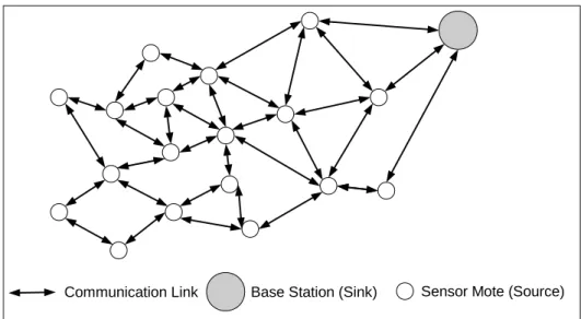
IGURES1.1 A typical multi-hop sensor network deployment. Intermediate sensor motes
are expected to report their own readings, as well as forwarding readings
received from other motes towards the base station via communication links. 3
2.1 Great Duck Island (GDI) deployment. . . 12
2.2 Intel Berkeley Research Lab (IBRL) deployment [11]. . . 16
2.3 Sensor data for node 15. Missing readings for over 5 minutes are left blank. . . 18
2.4 Temperature data of 15 nodes from the IBRL deployment. . . 19
2.5 Percentage of sensor data faults in the IBRL dataset. Faults mainly include
spike faults, stuck-at faults, and noise faults exhibited by the temperature and humidity sensors as well as clipping faults in the light readings. The number of outliers is negligible. . . 20
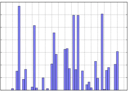
2.6 Number of clipping faults in the IBRL dataset. The histogram shows the
num-ber of anomalous readings caused by a clipping fault for each node. . . 21
2.7 Humidity readings spanning 3 days in October. Corrosions forming on the
connector to the sensor board on October 6 due to high humidity accounts for the erroneous readings. . . 23
2.8 Wind speed readings collected from two stations during the G´en´epi
deploy-ment. Data prior to October 19 are unusable due to a software bug in the wind sensor’s driver. . . 25
3.1 Types of anomalies in sensor network deployments and their corresponding
detection mechanisms. . . 35
3.2 Outlier readings of node 20 in the IBRL deployment. . . 47
3.3 Spike faults in different deployments. . . 49
3.4 Constant faults exhibited by node 6 in the SensorScope G´en´epi deployment. . . 50
3.5 Rain precipitation measured by two nodes (node 4 and 14) in the SensorScope
St. Bernard deployment. Node 14 exhibits a noise fault. . . 52
3.6 Noise faults in the IBRL deployment. . . 53
3.7 Clipping faults exhibited by node 20 in the IBRL deployment. The light
read-ings clipped at the highest peak are outside the range of possible ADC values. 56
3.8 Compromise data behaviors during lab deployment. Node 8 emits normal
tem-perature readings and is shown as a reference to compare against compro-mise nodes (nodes 12, 17, and 20). . . 61
3.9 A demonstration of a sinkhole attack in sensor networks. . . 65
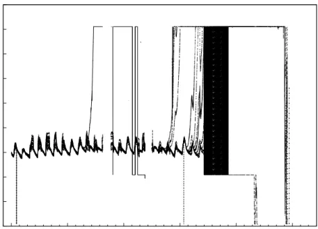
4.1 Various modeling techniques for spike faults exhibited by two sensor nodes in the IBRL deployment: nodes 6 and 18. For each node figure, the upper region plots the entire period of the spike fault followed by the steady be-havior of a stuck-at fault. The lower region plots the first two hours of the
spike period. . . 84
5.1 A taxonomy of data mining based anomaly detection approaches in wireless sensor networks . . . 93
5.2 Clustering-based and SVM-based data-centric anomaly detection in wireless sensor networks . . . 95
5.3 A scatter plot of the temperature and humidity readings from a 4-hour win-dow of readings (starting March 1) obtained during the IBRL deployment. Anomalies shown in the figure are elliptical anomalies discussed in [103] . 96 5.4 Detecting anomalies with ABANDON . . . 111
5.5 The detection error of the classifier using all three statistical features (highest gradient, temporal deviation, data range) over all sensing modalities (tem-perature, humidity, light). False negatives are eliminated at iteration 12. In this specific experimental run, there were no false positives since the very first iteration. . . 119
5.6 The first two hours of training data during the experimental deployment. The black lines correspond to readings from normal nodes. . . 122
5.7 The first two hours of testing data during the experimental deployment. Acous-tic signals exhibited one outlier reading over the 2-hour period (at 3:50 am). 123 5.8 Accuracy of the ensemble classifier after 100 iterations using decision stump as the base classifier. . . 125
5.9 Classification accuracy at 100 iterations. The learning process suffers from over-fitting for largerTp whenλis set too small. . . 126
5.10 Accuracy of the ensemble classifier after 100 iterations using decision trees as base classifiers. . . 126
6.1 A sensor network deployment leveraging a collection tree-like protocol such as CTP [37] . . . 132
6.2 Block diagram of the proposed online data-centric anomaly detection frame-work for sensor netframe-work deployments . . . 135
6.3 Online feature extraction and collection (β = 10,λ = 2) . . . 139
6.4 Functional block of the SNMiner toolkit . . . 150
6.5 SNMiner graphical user interface. . . 152
6.6 Detection errors for different values of β. Three statistical features were ex-tracted (temporal deviation, data range, and highest gradient). Errors are recorded after 300 boosting iterations. . . 153
6.7 Resulting ADTree classifier when β is set to 20 during simulation (refer to Figure 6.6). Number of iterations = 65. . . 154
6.8 Detection error when extracting all three features and using all three sensing modalities during the experimental deployment of 22 nodes. It takes 7 iterations to achieve a perfect detector. . . 156
6.9 The resulting ADTree classifier when all features are extracted over all sensing modalities during the experimental deployment. Boosting stops at iteration 70. (Figure 6.8). . . 156
L
IST OFT
ABLES1.1 Popular Commercial Sensor Platforms . . . 2
2.1 Summary of The Existing Deployments Discussed In This Chapter . . . 30
2.2 Summary of Anomalies Prevalent In The Deployments Discussed In This Chapter 33 3.1 Network Failures, Their Root Causes, and Possible Detection Approaches . . . 42
3.2 Node Failures, Their Root Causes, and Possible Detection Approaches . . . 46
3.3 Measurement Faults, Their Root Causes, and Detection Features . . . 58
3.4 Malicious Network Behaviors, Attack Characteristics, and Possible Detection Approaches . . . 71
4.1 A Set of All Outliers In The IBRL Dataset Prior To Battery Voltage Drops Under 2.40 Volts . . . 82
5.1 Anomaly Detection Schemes Discussed in This Section . . . 108
5.2 Summary of Extracted Statistical Features . . . 114
5.3 Compromise Data Behaviors (Training Phase) . . . 122
5.4 Compromise Data Behaviors (Testing Phase) . . . 123
5.5 Test Errors of The Evaluated Classifiers . . . 127
6.1 A Summary of Anomaly Models . . . 137
6.2 Injected Anomalies During The Training Phase (Simulation) . . . 153
6.3 Injected Anomalies During The Testing Phase (Simulation) . . . 153
6.4 Injected Anomalies During The Training Phase (Real-World Experiment) . . . 155
6.5 Injected Anomalies During The Testing Phase (Real-World Experiment) . . . . 155
6.6 Comparison of Total Complexities Per Node . . . 161
6.7 Description of Parameters Used In Table 6.6 And Section 6.5.4 . . . 161
A
CKNOWLEDGMENTSFirst and foremost, I would like to express my deepest gratitude to my advisor and friend Professor Bin Wang. Dr. Wang has been my mentor for six wonderful years. Work-ing together throughout my Master’s led me but to accept a great opportunity of pursuWork-ing a PhD under his supervision. He did not only believe in my research ideas, but also helped me take them to the next level, that being through delightful conversations, constructive feedback, and his tremendous assistance in proper formation of my thoughts. I truly owe him for his generous support, his dedication as my mentor, and after all for his trust in me and my work.
Second, I am very grateful to Dr. Yong Pei who supervised my very first sensor net-works project, and later gave me the opportunity to be his assistant in mentoring a senior design project. The skills that I acquired when working on these projects were those that minimized the time I spent implementing the prototypes discussed in this dissertation. Dr. Pei has been very caring, patient, encouraging, and always ready to give me an advise on different aspects of my life and career. I always enjoyed the numerous conversations we had about various subjects.
spent together discussing improvements and suggestions to the presentation of this re-search. Dr. Chen is very knowledgeable and I am fortunate to have him on my PhD committee. In addition, I would like to thank Dr. Shu Schiller for being a member of my PhD committee and for her invaluable suggestions pertaining to real-world applications.
My extreme gratitude goes to my father Rimon, my mother Linda, and my brothers Wadie, Rami, and Marco. Them believing in me was my key to completing this disserta-tion. I remember the days when a single conversation with my father would turn frustration into ambition and fatigue into excitement.
Last but not least, I would like to thank my colleague and friend Dr. Tao Zhang for introducing me to the field of machine learning. I had a great time working with him at the Broadband, Mobile and Wireless Networking Research Lab.
To my parents, for their love and everlasting encouragement.
Chapter 1
Introduction
Over the last decade, real-life deployments of sensor networks have grown in numbers for various applications. Most of these deployments have helped decision makers better under-stand their targeted environments by analyzing the data collected from a large number of unattended sensors. A typical deployment of a wireless sensor network (WSN) consists of several tens or hundreds of low-power low-cost tiny devices equipped with sensor boards capable of measuring several phenomena. These devices, usually called sensor motes, are also equipped with wireless communication modules that enable them to communicate with each others. Table 1.1 shows the characteristics of some sensor platforms (i.e. motes) popularly used in sensor network deployments. Two types of communication paradigms are possible: (a) a simplified single-hop communication where every sensor mote commu-nicates directly with a base station. A base station is a more powerful node which may further process and then relay messages towards a connected PC, and (b) a more complex multi-hop communication paradigm that involves forwarding messages from sensing nodes to the base station with the help of other intermediate sensor nodes in the network (see Fig-ure 1.1). The base station node is sometimes called the “sink” while other nodes in the network are referred to as “source nodes.”
Table 1.1: Popular Commercial Sensor Platforms
Name Image Manufacturer Processor Program/FlashMemory MemoryData ExternalFlash Radio Frequency BatteryType OS/VM LanguagesProg.
TelosB
MEMSIC
8MHz TI MSP430 48Kbytes 10Kbytes 1Mbyte 2.4GHz
2x AA TinyOS nesC MICA2 ATmega128L 128Kbytes 4K bytes 512Kbytes 868/916 MHz MICAz 2.4GHz IRIS ATmega12818MHz 8bit
8Kbytes TinyOS, MoteRunner VM nesC, Java/C# XM1000 advanticsys MSP430f26188MHz TI 116Kbytes
1Mbyte TinyOS, Contiki nesC, C Tmote Sky Sentilla 8MHz TI MSP430 48Kbytes 10Kbytes
SunSPOT ORACLE 400MHz 32bit AtmelAT91SAM9G20 8Mbytes 1Mbyte
-Li-Ion
Recharge-able
Squawk VM Java ME Waspmote Libelium 8MHz ATmega1281 128Kbytes 8Kbytes +4Kbytes SD Card2Gbytes 868/900MHz,2.4GHz
Auxiliary Recharge-able None C++ Imote2 MEMSIC (Intel-licensed) 13-416MHz PXA271 XScale 32Mbytes 256Kbytes + 32Mbytes -2.4GHz 3x AAA /
Li-Lon TinyOS nesC iSense
Core Module 3
Coalesenses 4-32MHz 32bit RISCController 512KbytesShared 128KbytesShared - PluggableResourcesiSense Firmware C++ TinyNode Shockfish TI MSP430 48Kbytes 10Kbytes 512Kbytes 433 MHz,
868MHz, 915 MHz Pluggable
Resources TinyOS nesC
One of the very first successful deployments of sensor networks took place at the Great Duck Island [123]. Researchers used data collected from environmental and occupancy sensors laid inside nests (burrows) to better understand the micro-climate surrounding seabirds, observe weather conditions during the breeding season, and measure the occu-pancy period of seabirds during incubation. The quality and accuracy of the collected sen-sor data was a major concern. To achieve higher fidelity in the data, appropriate packaging was necessary to protect the sensors from harsh environmental conditions. Without pack-aging, batteries may rapidly discharge or sensors may totally fail due to their exposure to chemicals such as carbon dioxide. The latter conditions can result in sensor faults that may highly degrade the quality of the sensor data. Even with the existence of appropriate pack-aging, sensors might still experience natural unknown faults or calibration drifts impacting the confidence in the generated sensor readings. As another example of an early success of sensor networks is the Redwood Forest deployment [126]. In this deployment, 33 sensor
Figure 1.1: A typical multi-hop sensor network deployment. Intermediate sensor motes are expected to report their own readings, as well as forwarding readings received from other motes towards the base station via communication links.
motes where placed at different heights of a 67-meter tree. Researchers collected tem-perature readings, relative humidity readings, and readings of solar radiation levels using Photo-synthetically Active Radiation (PAR) sensors to help better analyze the ecological conditions of a tree in the forest. The redwood forest deployment stressed the necessity of designing mechanisms to detect and correct sensor faults in a sensor network due to battery discharges and other possible causes regardless of perfect packaging and pre-deployment calibration.
Sensor networks are also susceptible to malicious threats if deployed in a hostile en-vironment. A malicious threat can vary from a simple passive eavesdropping attack to a total compromise of a sensor node. Sensor nodes, once compromised, can inject falsified readings into the network. Any inconsistent1 or malicious data behavior as a result from a security threat can degrade the trustworthiness, integrity, and/or accuracy of the sensor
1Previous research refers to inconsistent sensor readings that are far from the true value asoutliers,
anoma-lous,abnormal,faultyormaliciousdata. We will use all these terms interchangeably unless clearly stated in this dissertation.
data. The rise of the “Internet of Things” [6] has made WSNs even more appealing to the Internet community by connecting standalone sensor networks deployed in different geographical locations to the Internet and making sensor data accessible to authorized in-dividuals over the Web [1, 40, 50]. The level of confidence in publicly accessible sensors is still uncertain and there is a huge demand for data cleaning tools to filter out anomalous sensor readings.
To this end, researchers have proposed several approaches to detect inconsistencies and abnormal behaviors that can degrade the accuracy of the sensor data. Among those, ap-proaches rooted in the fields of machine learning and data mining proved to be effective. As part of this dissertation proposal, we explore a number of these techniques, their level of effectiveness, and their weaknesses. After that, we propose two new machine learning, i.e., boosting, based mechanisms for anomaly detection in sensor networks which can iden-tify both sensor data faults as well as compromised data behaviors. The major difference between the two proposed mechanisms is that the first detection mechanism is performed at the base station (centralized) whereas, in the second mechanism, the actual detection runs at the sensor level (online). The latter avoids communicating the large number of anomalous readings to the base station, and hence saving a tremendous amount of energy which is highly proportional to the communication cost. Furthermore, we design a toolkit that allows us to model anomalies and abnormal behaviors in a sensor network. Usually, researchers need to test the accuracy/effectiveness of their proposed anomaly detection al-gorithms. Anomaly models that are highly expressive are desirable due to the difficulty of obtaining a common ground truth necessary to evaluate against. In addition, with super-vised detection algorithms, it is essential to label anomalies according to their type. Highly
representative anomaly models may be injected to eliminate labeling errors during the la-beling process, or reduce tedious and error-prone efforts imposed by simple visual inspec-tions of the original dataset. The developed toolkit is also capable of extracting interesting statistical features and evaluating a number of supervised machine learning algorithms.
1.1
Motivations
This dissertation is driven by five major motives. First of all, a typical sensor network deployment is highly susceptible to various numbers of anomalous behaviors. Prior to de-signing a detection or preventive mechanism, it is very crucial to understand the frequency and characteristics of such behaviors. Once achieving a comprehensive study and analysis of anomalies prevalent in a sensor network deployment, researchers may focus on a spe-cific type of anomalous behaviors or rather design a generalized mechanism for detecting a good number of these anomalies. A number of researchers have identified the existence of such behaviors over the last decade and have designed detection and/or preventive mech-anisms addressing different types of anomalies. The fact that there is a large number of such proposed mechanisms imposes possible ambiguity of what is, indeed, being detected. We break this ambiguity by providing a taxonomy of anomalies prevalent in sensor net-work deployments and their corresponding detection mechanisms. Second, observing the anomalous behaviors prevalent in a number of successful sensor network deployments to date, has motivated us to re-think the existing mechanisms for ensuring the quality of the collected sensor data. There is a prompt need for anomaly detection mechanisms that iden-tify highly frequent sensor data faults towards avoiding quality degradation in the collected sensor data. Third, experimenting with a network of a few sensors at our lab has
strated the feasibility of simulating compromise behaviors in a sensor network with very little effort. A node, once compromised, can emit falsified readings, alter other nodes’ read-ings, or launch a security attack of any kind. This may render sensor data untrustworthy and unusable by application end-users who seek meaningful rather trustworthy inferences. Thus, there is also a high demand for anomaly detection mechanisms that can identify and eliminate compromise data behaviors to avoid lack of trust in the collected sensor data and/or data integrity vulnerabilities. Fourth, given the fact that sensor nodes are resource-constrained largely because of the lack of a continuous energy source and the small size of data and program memory spaces, it is crucial to design detection algorithms that take into account such characteristics if such mechanisms are to be deployed at the sensor level. Last, there is a lack of sensor network tools which facilitate the modeling of faults and malicious behaviors in a real-world sensor network deployment. The combination of ar-tificially injected but highly expressive anomalies coupled with real sensor data provide a more realistic sensor network model compared to purely synthetic datasets or publicly ac-cessible anomaly-free datasets. This drives us to develop a GUI tool, we call SNMiner, for that purpose. The development of SNMiner was also indirectly influenced by the lack of a standalone platform for rapid experimentation and evaluation of a machine learning based detection model under examination.
1.2
Thesis Objectives and Contributions
The ultimate objectives of this dissertation are summarized here: (i) Improving sensor data acquisition schemes in order to enhance the quality of the collected sensor data in the pres-ence of various anomalies; (ii) Providing a self-organizing sensor network that takes
pro-active measures in case of fault/compromise detection excluding erroneous sensor readings from calculations; (iii) Facilitating the machine learning process by building a responsive sensor network platform willing to train itself in the face of sensor faults and/or malicious behaviors; (iv) Achieving all of the above while maintaining an energy consumption of the sensor nodes nearly commensurate with that without employing any sort of quality assur-ance measures.
Our major contributions are summarized as follows. First, we put together a compre-hensive study of anomalies prevalent in current and futuristic sensor network deployments. There has been similar studies and surveys in the literature regarding anomalies in sensor networks. However, to the best of our knowledge, up to this moment none has provided a rather complete view of the nature of anomalous behaviors and none has intensively an-alyzed each of these behaviors. Second, we survey the literature in an attempt to provide a taxonomy of machine learning based anomaly detection techniques in sensor networks. We then propose a centralized data-centric anomaly detection technique borrowing from the field of machine learning and data mining. The technique employs a supervised en-semble learning algorithm called Adaptive Boosting (AdaBoost [35]) which relies on a combination of base classifiers to reduce the classification error and hence improving the accuracy of the ensemble classifier. We have shown that the technique yields a low number of false positives while being able to detect a large number of data-centric anomalies in a sensor network deployment. We further propose an on-line data-centric anomaly detection framework for sensor networks. This framework takes into consideration the high energy consumed by communicating sensor readings all the way to the base station. It solves this issue by running the detection at every sensor node in the network. It also employs an
online feature extraction mechanism whereby simple statistical features are extracted on the fly, and therefore, sensor readings do not need to be stored in memory. As an essen-tial part to every supervised machine learning algorithm, sensor data need to be labeled in advance. However, labeling data by itself is tedious as it usually requires visual inspection of every single original data point. Therefore, as a better alternative, we design highly ex-pressive anomaly models that represent measurement faults in existing real-world sensor datasets, possible events, as well as compromise data behaviors common in hostile deploy-ments. Anomaly modeling/injection, feature extraction, and algorithm accuracy evaluation, all were implemented under a unified toolkit called SNMiner.
1.3
Thesis Organization
The rest of the dissertation is organized as follows. The next chapter emphasizes the need for an anomaly detection mechanism by laying down a number of existing sensor net-work deployments and identifying instances of anomalies prevalent in such deployments. Chapter 3 provides a taxonomy of anomalies prevalent in sensor network deployments. Corresponding detection mechanisms are also being discussed. In Chapter 4, we design data-centric anomaly models which are highly representative of sensor data faults, compro-mise data behaviors, as well as possible events. Chapter 5 begins by surveying a number of existing machine learning based data-centric anomaly detection schemes for sensor net-works. In the same chapter, we propose a novel data-centric anomaly detection framework also rooted in machine learning which is capable of detecting both measurement faults as well as compromise data behaviors with low false positives. An online version of the later is proposed in Chapter 6. At the end of the same chapter, we present the design goals of the
SNMiner toolkit which was used frequently during this work. Finally, Chapter 7 concludes the dissertation.
Chapter 2
Prevalence of Anomalies In Real World
Deployments: The Need For Detection
Mechanisms
Sensor network deployments have enabled automated data collection at a finer granularity compared to human-centric sparse deployments of traditional telemetric data loggers, driv-ing scientists or application administrators to draw better conclusions from the collected sensor data. However, this fine granularity cannot be achieved in the presence of failing nodes, frequent network failures, and/or potentially malicious network behaviors. More-over, given a perfect and secure network with long-lived sensor nodes, finer-grained data samples may still not guarantee the quality of reasoning during the decision making process unless the sensor dataset is fault-free. Unlike traditional devices, wireless sensor motes are resource-constrained battery-powered devices equipped with few on-board sensors which are susceptible to failures, and batteries cannot always be reliably recharged. Over the years, sensor network deployments have materialized a large number of monitoring and event-detection applications. Examples include monitoring weather conditions [122, 126], habitat monitoring and wildlife tracking [5,119,122], monitoring of health conditions, flood detection [50], fire detection [75], volcano monitoring [131], structural health
monitor-ing [61], monitormonitor-ing the micro-climate inside greenhouses [4], monitormonitor-ing voltage usages at the micro-grid [22], monitoring water quality [106], measuring the quality of perish-able food and medicine [10], and tracing and verification of goods at different phases of the supply chain [10]. Researchers and decision makers have observed several anomalous patterns ranging from functional failures to pervasive sensing faults in most of these de-ployments. In this chapter, we discuss a few of these deployments to emphasize the need for an anomaly detection mechanism. Towards the end of the chapter, Table 2.1 compares the existing deployments we discuss here while Table 2.2 summarizes the different obser-vations sought in such deployments which revealed a number of anomalies.
2.1
Great Duck Island (GDI)
2.1.1
Overview
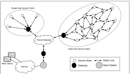
The GDI project [122] serves as one of the earliest proof-of-concept sensor network deploy-ments. The main purpose of this deployment was to help ecologists study the distribution and abundance of Leach’s Storm Petrels (a type of seabird species) at the Great Duck Island, Maine. The system deploys a multi-tier architecture (Figure 2.1) where one or more sensor patches are located at the lowest tier and the higher tier forms a transit network of gateways connecting the sensor patches to the remote base station(s). Each sensor patch is comprised of burrow motes equipped with temperature, humidity, and non-contact infrared tempera-ture sensors to monitor the occupancy of nesting burrows, and weather motes to measure the surface micro-climate using temperature, humidity, and pressure sensors. There were two types of deployments for sensor patches (with incremental installments): a single hop network of 49 Mica2Dot [118] motes running TinyOS [124] each of which samples
Figure 2.1: Great Duck Island (GDI) deployment.
ings every 5 minutes, and a multi-hop network of 98 motes with data sampled every 20 minutes. In addition, a verification network of in-burrow cameras was also deployed to obtain ground truth for occupancy verification by collecting 15-second movies every 15 minutes. The deployment operated over 115 days during the summer and autumn of 2003 and covered an ellipsoidal area of 221 by 71 squared meters. To protect the electronics from severe environmental conditions such as flooding or rain, the internal structure of motes was entirely covered with O-rings and conformal coatings. On-board sensors, however, needed to be exposed to the outside world to preserve their sensing capabilities.
2.1.2
Observations
Data Yield
Data yield is the ratio between the number of data points successfully delivered to the base station and the expected number of data points generated by all nodes in the network. During the multi-hop deployment, several failures (anomalies) were spotted that resulted in a low data yield. For instance, five burrow motes stopped reporting only after 5 days of
the deployment. This was due to rapid depletion of their batteries. Another example was the failure of gateways or the transit network accounting for a sensor data yield of merely 28%. In addition, the GDI deployment indicated that adequate packaging and efficient mote placement is essential: only 78 motes were recovered out of 150 devices as some were moved by animals and most of the recovered motes had their antennas removed or shortened by animals, eventually causing the node to fail to report its readings.
Measurement Faults
The GDI multi-hop deployment and an earlier deployment of a single hop network in the year 2002 [122], in which sensor motes also measured ambient light levels and sensor readings were sampled every 70 seconds, revealed that sensors may frequently malfunc-tion and provide erroneous or abnormal measurements due to various reasons discussed in Chapter 3. For example, during the 2002 deployment, about half of the temperature and humidity sensors reported faulty readings. This was mostly due to water contacts result-ing in short circuits. A faulty temperature readresult-ing manifested itself in a persistent readresult-ing
of 0◦C, whereas an anomalous humidity reading was either higher than 150% (out-lier)
or very small. The temperature sensor most often never recovered while humidity sensors which reported high spikes recovered after they dried up. Humidity sensors with very small values were also correlated with permanent node outages: 55% of motes exhibiting this be-havior failed within 2 days [123]. In addition, wet sensors in general caused the battery level to drop drastically. Light sensors, on the other hand, reported reliable readings most of the time with the few exceptions when there was a spike usually correlated with tempera-ture/humidity faults. Both deployments—single and multi-hop—showed that the operating
voltage threshold is 2.7V when using 2-AA alkaline batteries while using a lithium battery maintained a constant voltage, and sensor calibration, although time consuming, is essen-tial before deployment. Some of these facts have motivated researchers to design new mote architecture [96] which is more solid in face of sensor failures (e.g., cuts the power line to the failed humidity sensor when detected) and lasts longer (e.g., the operating voltage threshold is 1.8V).
2.2
Redwood Forests
2.2.1
Overview
A multi-hop network of Mica2Dot TinyOS-powered sensor motes [126] have replaced tra-ditional data loggers in the redwood forests of Sonoma, California. Motes were attached to the west side of a 70-meter tall redwood tree at approximately 2-meter spacing. Each mote was equipped with temperature, humidity, and two PAR sensors (photo-diodes) to mea-sure the micro-climate surrounding the tree. The network operated over 44 days during the Spring of 2004 and collected readings at a sampling rate of 5 minutes. The collected data helped biologists draw conclusions regarding the moving gradients inside the structure of the tree due to variations of the different phenomena over the tree volume. Packaging included a white skirt cover to protect the internal electronics from water and wind but still exposed the sensors to the environment to preserve their sensing capabilities. To be able to access the data from the outside world, a Stargate [121] gateway was placed at the bottom of the tree which stored sensor readings received over the multi-hop network into a TASK [11] database server.
2.2.2
Observations
Data Yield
The entire network collected only 49% of the total sampled data points. Network and node failures were the underlying reasons behind such a low yield. The gateway node suffered outages at the beginning of the deployment while five nodes stopped reporting during the second week. Researchers of the Redwood Forests deployment emphasized the need for network monitoring tools that can detect and report an abnormal behavior once it occurs. Measurement Faults
By analyzing the data, researchers have found several anomalous readings. For example, some sensor motes running on a low battery produced erroneous readings where others reported readings outside of the normal range (e.g., humidity readings above 100 %RH). The latter is an example of a clipping fault as will discuss in Chapter 3. Since battery failures accounted for most of the anomalies, a simple anomaly detection and filtration algorithm was applied. Sensor readings, reported when the mote’s voltage was outside the range 2.4V-3.0V, were deleted. In addition, humans were involved to remove motes which reported unexpected readings. This deployment has shown that physical installation (e.g., orientation) of sensor motes is very critical and calibration is inadequate to improve the fidelity of the data and other techniques are needed. A time consuming calibration of the humidity and temperature sensors resulted in only slight improvements.
Figure 2.2: Intel Berkeley Research Lab (IBRL) deployment [11].
2.3
Intel Berkeley Research Lab (IBRL)
2.3.1
Overview
Researchers at the Intel Berkeley Research Laboratory (IBRL) deployed an indoor net-work of 54 Mica2 and Mica2Dot motes in March 2004 [11]. Every 30 seconds, motes collected temperature, relative humidity, light, voltage, and topology information. The in-tention behind this deployment, which lasted for about 30 days (720 hours), was to verify the capability of the Tiny Application Sensor Kit (TASK) services in keeping the network alive over extended periods of time, and to provide the sensor network community with a publicly accessible sensor dataset allowing developers and other researchers to experi-ment with. The dataset acts as a benchmark to evaluate and compare anomaly detection algorithms against each others. The deployed motes formed the multi-hop network shown in Figure 2.2. The base station is the node with ID 0 and the farthest nodes at the upper left corner (e.g., node 51) are about 10 hops away from the base station. Sensor nodes ran TinyDB which is part of the TASK sensor kit. TASK also provided visual tools for
inspecting the quality of data and the status of the network.
2.3.2
Observations
Data Yield
The entire IBRL sensor dataset [19] contained 2,313,153 entries pertaining to only about half the expected number of entries. Each entry corresponds to a packet or sample received from one of the deployed sensors. Each packet contains the sampling date, sampling time, sequence number (epoch), node id, temperature reading, humidity reading, light reading, and the voltage level.
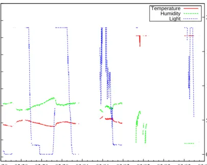
IBRL researchers found that 4 nodes failed after the first few days for unknown reasons. Even before failing, a high number of packet loss was observed. For example, for a little more than 8 hours starting 11:24 pm on March 1, packets from node 15 were not delivered to the base station most likely due to network contention or interference. The plot of node 15 data in Figure 2.3 shows missing sensor values over the lifetime of the node1. The rest of the motes were able to successfully transmit 30% to 82% of their packets over the lifetime of the deployment. In addition to the previous findings, we observe that the entire network has gone offline for two intermittent days. Although this may seem as a correlation of packet losses across sensors, this is not the case over the entire deployment [11]. The two intermittent days of complete loss may be due to a very high network contention or a base station breakage. The loss of sensor readings, however, seems to be highly correlated (a lost packet would result in total absence of all sensor readings). It is also worth mentioning that in the IBRL deployment, three nodes were potentially deployed later after the very first deployment of the original 54 nodes. They may also have been deployed initially but
1Missing periods are measured using a time gap of 5 minutes.
-20 0 20 40 60 80 100 120 140 160 02/28 00:00 02/28 12:00 02/29 00:00 02/29 12:00 03/01 00:00 03/01 12:00 03/02 00:00 03/02 12:00 03/03 00:00 03/03 12:00 03/04 00:00 0 500 1000 1500 2000
Temperature (Celsius) / Humidity (R%)
Light (Lux)
Time
Temperature Humidity Light
Figure 2.3: Sensor data for node 15. Missing readings for over 5 minutes are left blank. never reported any packets until too late in the deployment time for unknown reasons. It seems like the three nodes rebooted themselves (or were physically reset) as the sequence numbers did not always follow a sequential order.
In addition to total loss of packets, some nodes have reported packets with missing sensor values. Several packets (i.e., samples) from node 5 were delivered to the base sta-tion intermittently until March 3. However, the sensor readings were completely missing due to unknown reasons. From node 57, only 3 packets were delivered during the entire monitoring period, one of which had only a single sensor reading (humidity reading). Measurement Faults
Rajasegarar et al [104] have analyzed the IBRL set for data anomalies. They found that node 14 reported few anomalous readings (i.e., anomalous temperature and humidity) within a four-hour window starting midnight March 1. Within the same time window,
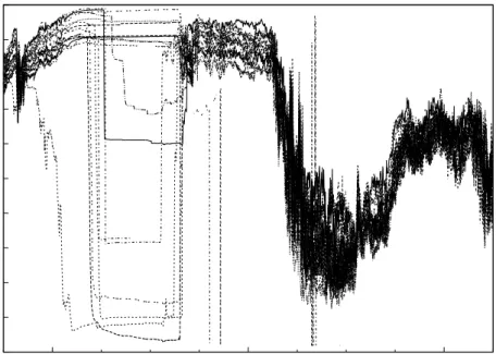
-40 -20 0 20 40 60 80 100 120 140
Feb 28 Mar 06 Mar 13 Mar 20 Mar 27 Apr 03
Temperature (
°
C)
Date
Figure 2.4: Temperature data of 15 nodes from the IBRL deployment.
node 37 reported anomalous readings at all times (i.e., anomalous node). It is believed that the reason behind the total anomalies of node 37 is its physical placement close to the kitchen (always higher temperature and humidity) and the unusual interference at the corner where node 14 is located accounts for its slightly erroneous behavior. In addition to anomalies resulted from nodes 14 and 37, other forms of fault were observed in [88]. For example, nodes 24 and 32 as well as other spatially correlated sensor nodes experienced clipping faults in the light readings over the course of the month. Clipping occurred in the middle of the day when the light sensor could not read values exceeding the limits of the analog to digital converter (ADC). As in the redwood forests project, due to low battery levels, some sensors have also shown abnormal behaviors that manifested themselves as spikes followed by a “stuck-at” fault as referred to in [88]. In the latter work, researchers have found that 20% of the total temperature readings were faulty. Figure 2.4 plots the tem-perature data measured by 15 nodes in the IBRL deployment. The figure reveals a number
0 0.2 0.4 0.6 0.8 1 1.2 1.4 3 6 9 12 15 18 21 24 27 30 33 36 39 42 45 48 51 54 57
Percentage of Anomalies (Faults)
Node Id Temperature
Humidity Light
Figure 2.5: Percentage of sensor data faults in the IBRL dataset. Faults mainly include spike faults, stuck-at faults, and noise faults exhibited by the temperature and humidity sensors as well as clipping faults in the light readings. The number of outliers is negligible. of faulty readings that manifest themselves as spikes, noise, outliers, and stuck-at faults. We will discuss the characteristics of such faults in the coming chapter. Since temperature and humidity readings are very highly correlated, one can imagine a similar plot for the humidity data. Notice that the majority of the temperature readings are spatially correlated (a node’s temperature reading is close to its neighbors’ readings at a time). Temperature readings are also temporally correlated within a short time window.
Figure 2.5 measures the frequency of faulty readings in the IBRL dataset. A number of sensor nodes (node 18, 29, 30, 32, 46, and 50) can only leverage 47% to 57% of its overall collected temperature and humidity readings. The rest of the readings are faulty and may be harmful to the decision making process. Temperature and humidity sensors exhibit spike, stuck-at, and noise faults whereas light sensors suffer from clipping. Figure 2.6 shows the actual number of clipping faults in the IBRL dataset. About half of the sensor nodes exhibit
0 2000 4000 6000 8000 10000 12000 14000 3 6 9 12 15 18 21 24 27 30 33 36 39 42 45 48 51 54 57
Number of Clipped Readings
Node Id
Figure 2.6: Number of clipping faults in the IBRL dataset. The histogram shows the num-ber of anomalous readings caused by a clipping fault for each node.
this behavior.
2.4
SensorScope
2.4.1
Overview
The SensorScope system [50], developed at EPFL (Swiss Federal Institute of Technology Lausanne), underwent 7 outdoor deployments over a span of three years (2006-2008) in different locations in Switzerland at a scale ranging from 6 to 97 weather stations. Each weather station is equipped with a well-packaged Shockfish TinyNode [85] and nine envi-ronmental sensors which measure a handful of envienvi-ronmental observations every 2 minutes (e.g., air humidity and temperature, soil moisture, rain precipitation, solar radiation, water-mark, and wind direction/speed). Sensor motes receive power from an NiMH battery that is rechargeable via a solar panel located at the top of the station. The two most significant
ployments took place at: (i) a rock glacier located at 2500-meter high on top of a mountain in G´en´epi, Switzerland, and; (ii) the 2400-meter high Grand Saint Bernard pass located between Switzerland and Italy. In both cases, weather data were collected over a multi-hop network of weather stations and transmitted by a GPRS-enabled gateway to a database server. Data are publicly accessible over the Internet and can be viewed using popular Web interfaces (i.e., Google Maps, Microsoft’s SensorMap). The G´en´epi deployment had 16 stations scattered over 500x500 meters area reporting weather data during August-October 2007 (60 days). Detecting floods and rock falls in the area was the main reason behind this deployment as the mountain is a source of mud streams and rock releases due to the melt-ing of underlymelt-ing permafrosts. The second deployment consisted of 17 stations deployed in September 2007 for 45 days on a 900-meter long line over the Bernard pass to prevent avalanches [7].
2.4.2
Observations
Data Yield
There were a few missing data points during both the G´en´epi and Grand St. Bernard de-ployments. As an example, during the former deployment, station 7 did not report any readings over more than a week during the middle stage of the deployment. Mostly, hard-ware failures due to short circuits accounted for this behavior. As reported in [8], the total number of data points collected from the two deployments was 5800000 and 4300000 re-spectively. This results in a data yield of approximately 93% and 87% rere-spectively. In order to be able to monitor the network, SensorScope collected status packets in addition to data packets. Status packets carried energy, network, and topology information that can
0 10 20 30 40 50 60 70 80 90 100
Oct 06 Oct 07 Oct 08
Relative Humidity (R%)
Date
Figure 2.7: Humidity readings spanning 3 days in October. Corrosions forming on the connector to the sensor board on October 6 due to high humidity accounts for the erroneous readings.
help network administrators identify potential network and node failures. Measurement Faults
SensorScope researchers have pointed out several challenges associated with sensor net-work deployments. Some of the major challenges were: (i) packaging, (ii) calibration, (iii) detecting software bugs during deployment, and (iv) tracing unexpected failures. Sensor packaging is important but difficult. In both deployments, erroneous sensor readings were reported during cold and humid periods due to inadequate packaging. The latter allowed corrosions to form on the connector to the sensor board causing short circuits. This resulted in useless readings from all humidity sensors at G´en´epi mountain [8] on October 6 as seen in Figure 2.7. It also caused the rain sensor of station 14 at the Bernard pass [50] to report faulty precipitation values. The humidity sensor, a Sensirion SHT75 sensor, was embedded
within a stacked-plates structure and a small adapting circuit. Whereas, the wires were protected using epoxy resin. Calibration is required before, during, and post deployment. After packaging, sensors were pre-calibrated by comparing their values to a reference sta-tion over several days. During pre-calibrasta-tion, some temperature sensors reported an offset of over than 2◦C, which is much higher than the expected offset of 0.3◦C, and needed to
be discarded. Once deployed, some sensors such as the wind direction sensor should also be calibrated to avoid significant errors in their measurements. Finally, it is important to re-calibrate the sensors after deployment to flag faulty readings.
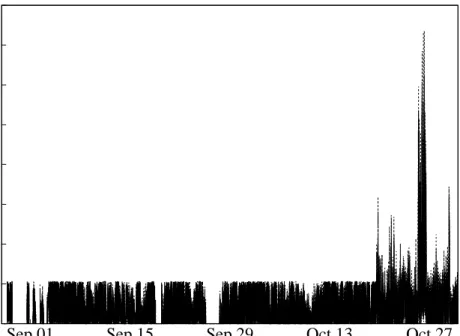
Despite the fact that the majority of software bugs are easily detected and fixed be-fore deployment and during indoor testing, some code bugs go undetected especially if configuration parameters are modified right before or during deployment. As an example, by observing the wind speed data of station 6 during the G´en´epi deployment, developers discovered a subtle bug in the wind sensor’s driver: an 8-bit counter was not adequate to store the number of revolutions the anemometer completes during one sampling period. The bug was not detected during pre-deployment testing since the sampling period was set much shorter (30 seconds). This bug affected all wind sensors alike, rendering the wind speed readings unusable over the period during which counter overflows were encountered. Figure 2.8 shows wind speed readings collected from two stations during the G´en´epi de-ployment. Clearly, all data before October 19 are useless.
Finally, uncorrelated sensor readings may be reported unexpectedly. In [8], authors joked about one occasion where one of the weather stations continuously generated un-correlated sensor readings (anomalous node), to find out that it was entirely covered with plastic wraps by construction workers to protect it from a near-by construction.
0 2 4 6 8 10 12 14 16
Sep 01 Sep 15 Sep 29 Oct 13 Oct 27
Wind Speed (m/s)
Date
Figure 2.8: Wind speed readings collected from two stations during the G´en´epi deploy-ment. Data prior to October 19 are unusable due to a software bug in the wind sensor’s driver.
We have seen that, although sensors were carefully calibrated, anomalies still occurred due to other issues mentioned above (i.e., inadequate packaging, software bugs, unexpected behaviors). In [112], for example, authors have identified SHORT faults (outliers) in three of the 31 weather stations deployed outdoor on the EPFL campus and it is not clear what caused such faults. Flagging and removing anomalies is usually done manually with hu-man intervention. Manual anomaly filtering is time consuming, therefore, SensorScope researchers have called for better approaches that rely on powerful off-line analysis and rapid on-line detection algorithms to filter out outliers and hence to ameliorate sensor data quality.
2.5
GreenOrbs
2.5.1
Overview
The GreenOrbs project [75, 82] aimed at monitoring the micro-climate and ecological trends in the forest. The collected sensor data support several applications including fire risk evaluation, biodiversity and forestry research, monitoring of carbon dioxide ab-sorbed by trees during the photosynthesis process, and estimation of canopy closure [82]. GreenOrbs deployments were carried out at several locations in the forest at a scale ranging from 50 nodes to 349 nodes during a recent deployment [114]. The long-term goal is to achieve a year-round kilo-scale sensor network deployment with 1000+ motes. The first deployment operated over 30 days starting July 2008 and consisted of 50 TinyOS-powered TelosB [96] motes scattered in a 20,000 meter squared forest at the campus of Zhejiang Agriculture & Forestry University, Hangzhou, China. The deployed motes formed a multi-hop network of 6-multi-hop diameter. The second deployment took place in March 2009 with 120 motes forming a 10-hop network. Since then, the network has been continuously expanded. The system employs the TinyOS conventional services for network-wide synchronization to enable duty cycling (FTSP [79]), reconfiguration (DRIP [125]), and sensor data collec-tion (CTP [37]). Motes collect temperature, humidity, light, voltage, and carbon dioxide (CO2) levels. The network also collects routing, neighborhood, and node statistics
infor-mation. The latter helps diagnosing the network to identify root causes such as link failures or any functional abnormal behavior in the network [114]. Each sensor mote runs on 2 AA batteries and is enclosed inside a plastic box to protect it from harsh environmental conditions such as rain. To maintain light readings close to the true illuminance values, the
top of the box is designed to be transparent, whereas holes on the sides of the box main-tain temperature and humidity values close to those outside of the box. Finally, the box is mounted on a bracket to protect it from wild animals.
2.5.2
Observations
Data Yield
At a scale of 330 nodes, GreenOrbs researchers found that the network yield dropped from 60% to 10% when changing the sampling frequency from 20 minutes to 66 seconds [75]. Further investigations revealed that the main reason behind packet losses was packet drops due to poor wireless channels or severe collisions. This accounted for 61.08% of all packet losses. Due to this severe case, about 10% of the nodes were forced to drop a packet 20 to 50 times after 30 failed retransmission attempts. The rest of the packet drops were due to forwarding queue overflows at the receiver side (i.e. severe data congestion). Ingress drops could also take place due to a software bug that leads to a locked memory state of the forwarding queue in CTP. All the ingress drops occurred on less than 5% of the nodes. In addition, a number of nodes never successfully reported data to the sink [75] due to software or hardware problems [80]. Routing loops, on the other hand, were considered silent failures that are hard to detect but can drastically hinder the network performance. Measurement Faults
Similar to previous deployments discussed above, calibration turned out to be very impor-tant but hard and time consuming. For instance, during a deployment test of 21 nodes [82], the maximum deviation of one light reading from another was 6KLux when all motes were placed under the same illuminance level and 8.41KLux when placed under different
nance levels. Light readings were used to estimate the canopy closure (i.e., the percentage of the ground area vertically shaded by overhead foliage). This shows how important it is to pre-calibrate the sensors before deployment to eliminate instrumental errors and deviations in the light readings between correlated sensors, and hence arrive at an accurate estimation. Despite packaging and calibration efforts, GreenOrbs researchers still identified frequent pervasive sensing faults [75].
2.6
VigilNet
2.6.1
Overview
As one last real-world example, we consider VigilNet, a sensor network deployment for target tracking and surveillance [44]. It is an example of an event-driven application. The major challenge of VigilNet is to accurately estimate the speed and location of an intruder (e.g., a vehicle) while keeping the entire system stealthy and energy efficient. Stealthiness is very important when motes are deployed in hostile environments and therefore, are vul-nerable to attacks. The size of a sensor node should be unobtrusively small and the network traffic should be minimized. Positioning sensor motes in hidden areas protects them from node compromise while minimizing network traffic reduces the chance of interception of RF signals and packet sniffing. In VigilNet, 70 Mica2 motes running TinyOS were de-ployed over a 280-feet long grassy road, 35 motes on each side of the road. The road may typically resemble a hostile area to be monitored. A sensor board is mounted on top of the mote and is capable of measuring magnetic fields generated by the movement of target objects, acoustic signals, motion, and distance of the object. The dual-axis magnetometer can sense slowly moving vehicles at a distance of approximately 8-10 feet. In addition,
few long-range gateways are deployed in the sensor field which are responsible for relay-ing traffic to a distant base station. The base station is attached to a portable device such as a laptop which, in turn, triggers two cameras in the sensor field when a movement is detected.
2.6.2
Observations
In order to precisely estimate the position of the moving vehicle, the number of faulty read-ings generated by the magnetometers, due to potential change of power state or hardware failures, should be minimized. VigilNet employs aggregation where a leader node fuses correlated magnetic readings from its group members and discards readings from deviat-ing members. The degree of aggregation (DOA), i.e., the number of group members, is a key parameter which controls the percentage of false positives (i.e., reporting an event while there is no vehicle in the vicinity of the sensor field) and false negatives (i.e., miss-ing reports of movmiss-ing vehicles). Without employmiss-ing aggregation, the false positive rate is very high (60%). False positives are eliminated if DOA is set to 3, i.e., a leader node fuses readings from three members before reporting an event to the base station. In ad-dition to on-line fault detection and elimination via in-network aggregation, VigilNet also applies off-line fault detection at the base station by analyzing the spatiotemporal correla-tion among consecutive events. Consequently, the base stacorrela-tion sends power-off signals to shut down misbehaving nodes.
Similar to the deployments discussed previously, VigilNet researchers have also advo-cated for software calibration to eliminate sensor drifts as much as possible before deploy-ment as well as repeated calibrations over time to adapt to changes in the environdeploy-ment.
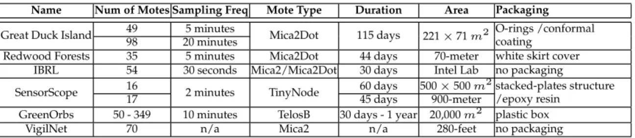
Table 2.1: Summary of The Existing Deployments Discussed In This Chapter
Name Num of Motes Sampling Freq Mote Type Duration Area Packaging
Great Duck Island 49 5 minutes Mica2Dot 115 days 221×71m2 O-rings /conformal
coating 98 20 minutes
Redwood Forests 35 5 minutes Mica2Dot 44 days 70-meter white skirt cover IBRL 54 30 seconds Mica2/Mica2Dot 30 days Intel Lab no packaging SensorScope 16 2 minutes TinyNode 60 days 500×500m
2
stacked-plates structure /epoxy resin
17 45 days 900-meter
GreenOrbs 50 - 349 10 minutes TelosB 30 days - 1 year 20,000m2 plastic box
VigilNet 70 n/a Mica2 n/a 280-feet no packaging
Unlike the deployments discussed above, however, sensor nodes in VigilNet are more vul-nerable to security attacks due to the nature of the application. For some experiments, which required a long duration of time, VigilNet researchers could not afford to deploy the system unattended due to security issues [44]. Nodes in VigilNet can also be easily compromised. Despite precise calibration and fault detection via on-line fusion and off-line analysis, node compromise can drastically affect the fidelity and trustworthiness of the vehicle detection estimate. Once a node is compromised, injecting falsified readings in a smart way may harm the aggregation process or even worse these readings become hard to detect off-line. Hence, anomaly detection algorithms should also be able to identify such behavior and potentially eliminate readings from compromised nodes. Furthermore, these algorithms should detect malicious network behaviors that may hinder the network performance (e.g., data yield, latency, etc.) or shorten its lifetime.
2.7
A Smarter Supply Chain
As can be seen, anomaly detection in existing sensor network deployments is a crucial challenge which needs to be addressed. Researchers have also envisioned future deploy-ments at a very large scale. As an example, Franklin et al [33] have envisioned a supply chain management (SCM) system, an example of a high fan-in (HiFi) system, where
sen-sor data are initially collected and cleaned at the receptor-level which constitutes a number of field deployable units (FDUs). A FDU has a network of sensors and a set of RFID readers. FDUs may be located at different places in the supply chain, including store shelves, store checkouts, and manufacturing lines. Data are then aggregated and smoothed by Stargate-like devices [121] at the second level (i.e., dock doors level). At the third level (i.e., warehouse level), sensor data are arbitrated and sensor streams are correlated across all devices by full-fledged centralized servers. The interior of the system constitutes the regional centers (fourth level) where data are validated, and the headquarters (fifth-level) at which data mining algorithms are run over the processed sensor data streams on the fly to foster the business decision making process and to provide better sales recommendations. A HiFi proof-of-concept prototype was proposed by the authors in [33] which constitutes three-levels of the main system’s hierarchy and uses TinyDB [78] for querying as well as TelegraphCQ [13], an adaptive data stream processor. The authors have also demonstrated the significance of pushing data cleaning and data reduction (i.e., aggregation) function-alities to the edges of the HiFi system. This calls for anomaly detection algorithms at the integrated WSN-RFID [109] end. The CSAVA (clean, smooth, arbitrate, validate, and analyze) process discussed in the paper incorporates several data processing tasks at the various levels of the HiFi system: cleaning, fault detection, anomaly detection, calibration, stream correlation, and event monitoring. Cleaning and smoothing are achieved by simple filtering queries; sensor readings with an RSSI (Received Signal Strength Indicator) higher than a certain threshold will be discarded, and if the number of readings over a time win-dow is less than a user-specified threshold, these readings are dropped. This calls for more advanced anomaly detection techniques at the receptor-level which may further improve
accuracy against erroneous and noisy sensor data, detect abnormal sensor activities, and avoid fail-dirty cases where sensor nodes fail to report correct readings due to a possibly drained battery.
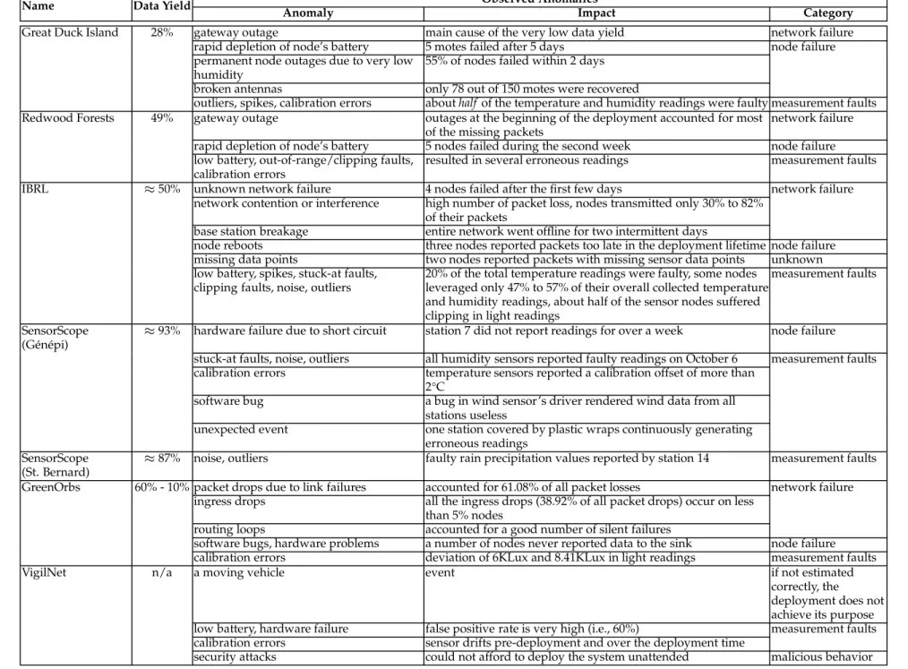
Table 2.2: Summary of Anomalies Prevalent In The Deployments Discussed In This Chapter
Name Data Yield Anomaly Observed AnomaliesImpact Category
Great Duck Island 28% gateway outage main cause of the very low data yield network failure rapid depletion of node’s battery 5 motes failed after 5 days node failure permanent node outages due to very low
humidity
55% of nodes failed within 2 days broken antennas only 78 out of 150 motes were recovered
outliers, spikes, calibration errors abouthalf of the temperature and humidity readings were faulty measurement faults Redwood Forests 49% gateway outage outages at the beginning of the deployment accounted for most
of the missing packets
network failure rapid depletion of node’s battery 5 nodes failed during the second week node failure low battery, out-of-range/clipping faults,
calibration errors
resulted in several erroneous readings measurement faults IBRL ≈50% unknown network failure 4 nodes failed after the first few days network failure
network contention or interference high number of packet loss, nodes transmitted only 30% to 82% of their packets
base station breakage entire network went offline for two intermittent days
node reboots three nodes reported packets too late in the deployment lifetime node failure missing data points two nodes reported packets with missing sensor data points unknown low battery, spikes, stuck-at faults,
clipping faults, noise, outliers
20% of the total temperature readings were faulty, some nodes leveraged only 47% to 57% of their overall collected temperature and humidity readings, about half of the sensor nodes suffered clipping in light readings
measurement faults
SensorScope
(G´en´epi) ≈
93% hardware failure due to short circuit station 7 did not report readings for over a week node failure stuck-at faults, noise, outliers all humidity sensors reported faulty readings on October 6 measurement faults calibration errors temperature sensors reported a calibration offset of more than
2°C
software bug a bug in wind sensor’s driver rendered wind data from all stations useless
unexpected event one station covered by plastic wraps continuously generating erroneous readings
SensorScope
(St. Bernard) ≈
87% noise, outliers faulty rain precipitation values reported by station 14 measurement faults GreenOrbs 60% - 10% packet drops due to link failures accounted for 61.08% of all packet losses network failure
ingress drops all the ingress drops (38.92% of all packet drops) occur on less than 5% nodes
routing loops accounted for a good number of silent failures
software bugs, hardware problems a number of nodes never reported data to the sink node failure calibration errors deviation of 6KLux and 8.41KLux in light readings measurement faults
VigilNet n/a a moving vehicle event if not estimated
correctly, the deployment does not achieve its purpose low battery, hardware failure false positive rate is very high (i.e., 60%) measurement faults calibration errors sensor drifts pre-deployment and over the deployment time
security attacks could not afford to deploy the system unattended malicious behavior
3
Chapter 3
A Taxonomy Of Sensor Network
Anomalies and Their Detection
Approaches
The previous chapter explored several real-world sensor network deployments and identi-fied instances of anomalies in each deployment. In this chapter, we systematically analyze the different types of anomalies prevalent in a sensor network, construct a taxonomy of such anomalies, and discuss potential detection mechanisms necessary to reveal the root causes behind each anomaly. Figure 3.1 illustrates three major types of anomalies that can exist in a sensor network deployment; (i) a natural fault; (ii) a malicious behavior; and (iii) an event. We discuss each category independently, pinpointing the possible root causes and the potential tools or mechanisms necessary to detect (and possibly recover from) all or a subset of these anomalies.
The chapter is organized as follows. Natural faults, malicious behaviors, and events are discussed in the next three sections. Having emphasized the demand for anomaly detection mechanisms in real-world applications and deployments of sensor networks, Section 3.4 summarizes the challenges of designing an anomaly detection algorithm for sensor net-works. Finally, we discus related work in Section 3.5 and conclude in Section 3.6.