A Computational Study of Flow Over a Wall-Mounted Cube in a Turbulent Boundary Layer Using Large Eddy Simulations

(1)

A Computational Study of Flow Over a Wall-Mounted

Cube in a Turbulent Boundary Layer Using Large

Eddy Simulations

by

Siddhesh Dilip Shinde

A dissertation submitted in partial fulfillment of the requirements for the degree of

Doctor of Philosophy

(Mechanical Engineering and Scientific Computing) in The University of Michigan

2018

Doctoral Committee:

Associate Professor Eric Johnsen, Chair Assistant Professor Jesse Capecelatro Associate Professor Kevin Maki Professor Joaquim Martins

(2)

(3)

Siddhesh Shinde siddhesh@umich.edu ORCID iD: 0000-0002-0378-6761

c

(4)

(5)

ACKNOWLEDGEMENTS

First and foremost I would like to express my immense gratitude and love towards my family, especially my parents, who taught me to be fearless and always motivated me to strive for excellence. This thesis would not have been possible without their support, for which I will forever be in their debt. I would like to express my deepest thanks to Dr. Eric Johnsen, my adviser, for this continued guidance and intellectual support during the course of my thesis. His advice has helped me excel in my research endeavor, and enabled me to perform at the best of my ability. I take this opportunity to thank Dr. Kevin Maki for his valuable inputs that have played a vital role in shaping my thesis objectives. I extend my thanks to my committee members Dr. Joaquim Martins, and Dr. Jesse Capecelatro for their thoughts and advice on my work. I would also like to thank Dr. Pooya Movahed for his contributions in developing the inflow boundary condition method.

My experiences at the University of Michigan have been invaluable in shaping my person-ality, and I am thankful for the memories I will cherish forever. I want to thank my colleague and dear friend, Suyash. Our research has progressed in tandem since the inception of my thesis, and I believe have gained a valuable friend for life. I want to thank all my friends including Vicky for co-founding “House of Bhaus”, Jovin for being the younger brother away from home, Sameer for his wit and delicious cooking, Nikhil for his Chai sessions, Prasad for his life lessons, Nitish for his anecdotes, Sumit for his social media skills, and Namit for his Bollywood enthusiasm. I truly believe my time at the University of Michigan would not have been nearly as fulfilling without the company of my friends in the Autolab. I am thankful to Brian for his house parties and science talks, TJ for his board problems and humor, Brandon

(6)

for this help with anything computer related, Mauro for proof-reading my documents, Marc for his research related inputs, Sam for his insights into French culture, Harish for his philos-ophy about life, Phil for sharing his DG wisdom, Kevin for his March madness enthusiasm, and Greg and Yang for all the OpenFOAM related help. Their presence made the Autolab a fun place to work and my graduate experience a pleasant journey. During my PhD I served on the board of Graduate Rackham INternational (GRIN) student organization. I want to thank everyone at GRIN for giving me the opportunity to contribute my bit to improving the graduate life experience of all international students on campus. I also worked with the Michigan Data Science Team (MDST) on exciting machine-learning projects, and I am grateful to them for this collaborative opportunity. Finally, I want to thank my undergrad friends from Sardar Patel College of Engineering (SPCE), Mumbai, India: Jugal, Kumar, Priyam, Ankit, Atharv, Chaithra, Parshva, Manalee, Pranav, Arati, Saurabh, Saumil, for all the adventures, love and craziness.

This work used the Extreme Science and Engineering Discovery Environment (XSEDE), which is supported by National Science Foundation grant number ACI-1053575.

(7)

LIST OF FIGURES

Figure

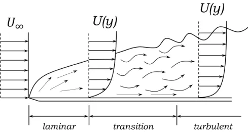
1.1 A schematic representation of laminar to turbulent boundary layer transition. 3 1.2 Mean turbulent boundary layer velocity profile normalized by the outer

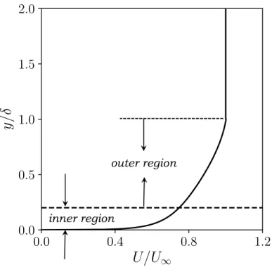
vari-ables. . . 5

1.5 Streamwise vortices produced by vane-type VGs from Cuvier [3]. . . 9

1.6 A type classification of flow control actuators from Cattafesta et al. [4]. . . 11

1.7 A schematic of synthetic jets from Cuvier [3]. . . 11

1.8 Forces acting on an automobile as a function of it’s speed from Barnard [5]. 12 1.9 Visualization of air-flow separation of the rear end of an automobile. Photo credit: NASA [6]. . . 13

1.14 Iso-surfaces of Q−criterion colored with vorticity magnitude for flow over a wall-mounted cube in a spatially evolving turbulent boundary layer. . . 20

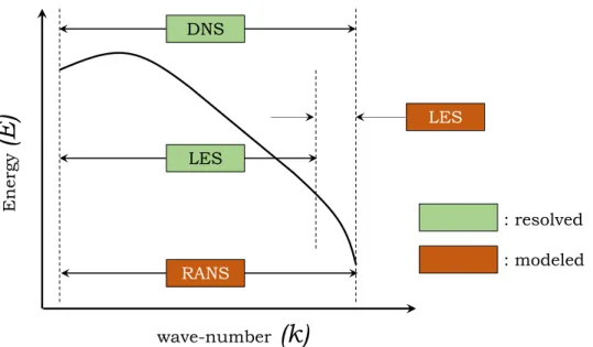
2.1 Schematic of the one-dimensional turbulent kinetic energy spectrum as a function of wave-number. . . 25

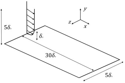
2.2 Flow configuration for validation of the inflow generator technique. . . 37

2.3 Span-wise average of Reynolds stress profiles at the inlet . . . 38

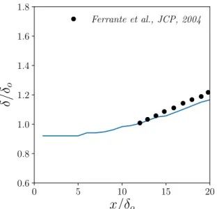
2.4 Mean quantities averaged in time and span-wise direction. . . 39

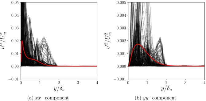
2.5 Reynolds stress profiles averaged in time and span-wise direction at different stream-wise locations. . . 39

(11)

2.6 Reynolds stresses at x/δo = 15 from the precursor simulation. Red curve is the mean, averaged in time and the spanwise direction. Black lines are the instantaneous profiles. . . 43 2.7 Machine-learned profiles of Reynolds stresses at x/δo = 15 from the

precur-sor simulation. . . 45 2.8 Results from main SETBL simulation on a flat plate using ML inflow approach. 46 2.9 Instantaneous velocity fluctuation profiles generated by the physics-based

approach and the ML approach. . . 47 2.10 Span-wise averaged profiles vs. normalized wall-normal coordinate (y) from

a SETBL on a flat plate using the ML approach. . . 49 3.1 Problem setup . . . 56 3.2 Computational grid for h/δo= 1.0. . . 57 3.3 Iso-surfaces ofQ−criterion colored with vorticity in the near wall region for

a cube with h/δo = 1.0 in a SETBL. . . 59 3.4 Skin friction coefficient (Cf) for different h/δo ratios. . . 60 3.5 Span-wise contours of streamwise component of the mean vorticity atx/h=

0.1,0.5 and 0.9 along the cube, with the cube outlined in black . . . 62 3.6 Mean pressure contours in the y −z plane at x/h = 0.5, with the cube

outlined in black. . . 62 3.7 Span-wise contours of stream-wise mean vorticity at x = 3h and 5h

down-stream of the cube. . . 63 3.8 Mean velocity and Reynolds stress profiles at y = 0.5h, x = 4h for h/δo =

1.0: ,u02_; _, _v02_; _,_w02_; _,_u0_v0_; _,_u0_w0_; _,

v0_w0_{. . . .} ₆₄

3.9 Mean velocity and Reynolds stress profiles in the centerplane and at z =h for h/δo = 1.0 atx= 4h: ,u02; , v02; , w02; , u0v0;

, u0_w0_; _, _v0_w0_{. . . .} ₆₅

3.10 TKE area density as a function of stream-wise location for different h/δo ratios. . . 67 3.11 TKE area density dependence on the normalized stream-wise coordinate. . 69 3.12 TKE production to dissipation ratio contours in the y−z plane at x/h =

0.5,2 and 5. . . 70 3.13 Contours of the production term and absolute value of the dissipation term

from the TKE budget ofh/δo = 1.0 in the center-plane. . . 72 3.14 Normalized span-wise averaged terms on the right hand side of the TKE

bud-get equation at x = 0.5h: , convection; , production; , turbulence transport; , viscous diffusion; , viscous dissipation;

, velocity-pressure gradient. . . 72 3.15 Normalized span-averaged terms on the right-hand-side of the TKE

bud-get equation at x/h = 3: , convection; , production; , turbulence transport; , viscous diffusion; , viscous dissipation;

(12)

3.16 Normalized span-averaged terms on the right-hand-side of the TKE bud-get equation at x/h = 6: , convection; , production; , turbulence transport; , viscous diffusion; , viscous dissipation;

, velocity-pressure gradient. . . 75

4.1 Problem setup. . . 82

4.2 Computational grid for w= 7h. . . 83

4.3 Skin friction coefficient vs. normalized stream-wise coordinate. . . 85

4.4 Normalized mean velocity vs. normalized span-wise coordinate at x= 5.5h in the stream-wise direction and y= 0.5h in the wall-normal direction. . . 87

4.5 Normalized Reynolds stresses vs. normalized span-wise coordinate at x = 5.5h and y = 0.5h. , u02_; _, _v02_; _, _w02_; _, _u0_v0_; , u0_w0_; _, _v0_w0_{. . . .} ₈₈

4.6 Normalized mean velocity vs. normalized wall-normal coordinate at x = 5.5h in the stream-wise direction and in the center-plane (z = 0). . . 89

4.7 Normalized mean velocity vs. normalized wall-normal coordinate at x = 5.5h in the stream-wise direction and at z =h in the span-wise direction. . 89

4.8 Normalized Reynolds stresses vs. normalized wall-normal coordinate at x= 5.5h in the center-plane (z = 0). , u02_; _, _v02_; _, _w02_; , u0_v0_; _, _u0_w0_; _,_v0_w0_{. . . .} ₉₀

4.9 Normalized Reynolds stresses vs. normalized wall-normal coordinate at x= 5.5h and z =h. , u02_; _, _v02_; _, _w02_; _, _u0_v0_; _, u0_w0_; _, _v0_w0_{. . . .} ₉₀

4.10 Span-wise contours of streamwise component of the mean vorticity atx/h= 0.1,0.5 and 0.9 along the cube, with the cube outlined in black. . . 91

4.11 Span-wise contours of streamwise component of the mean vorticity atx/h= 3 and 5 in the wake of the cube. . . 92

4.12 TKE area density as a function of the stream-wise distance for different inter-cube spacings. . . 93

4.13 Absolute value of TKE production to dissipation ratio contours in they₋z plane at x/h= 0.5,3 and 6, with the cube outlined in black. . . 95

4.14 Span-wise averaged TKE budget normalized using outer coordinates at x= 0.5h: , convection; , production; , turbulence trans-port; , viscous diffusion; , viscous dissipation; , velocity-pressure gradient. . . 97

4.15 Span-wise averaged TKE budget normalized using inner and outer coordi-nates atx= 3h: , convection; , production; , turbulence transport; , viscous diffusion; , viscous dissipation; , velocity-pressure gradient. . . 98

4.16 Span-wise averaged TKE budget normalized using inner and outer coordi-nates atx= 6h: , convection; , production; , turbulence transport; , viscous diffusion; , viscous dissipation; , velocity-pressure gradient. . . 100

A.1 Schematic of the problem setup. . . 113

A.2 Mean quantities averaged in time and the span-wise direction. . . 114 A.3 Normalized Reynolds stresses averaged in time and the span-wise direction. 114

(13)

B.1 Problem setup. . . 117 B.2 Mean velocity components and Reynolds stresses in the center plane for fully

developed turbulent flow around a wall-mounted cube in a channel . +: experimental result [11]; dashed line: one equation model [12]; dash-dotted line: localized dynamic one equation model [12]; pink line: our results with dynamic k−equation model. . . 119 C.1 Profiles of mean velocity (x-component) and Reynolds stress (xx-component)

for spatially evolving turbulent boundary layer flow around a wall-mounted cube withh/δo = 0.2. coarse mesh, medium mesh, fine mesh. 122 C.2 Profiles of mean velocity (x-component) and Reynolds stress (xx-component)

for spatially evolving turbulent boundary layer flow around a wall-mounted cube withh/δo = 0.6. coarse mesh, medium mesh, fine mesh. 123 C.3 Profiles of mean velocity (x-component) and Reynolds stress (xx-component)

for spatially evolving turbulent boundary layer flow around a wall-mounted cube withh/δo = 1.0. coarse mesh, medium mesh, fine mesh. 124 D.1 TKE budget terms in a turbulent boundary layer on a flat plate at a

(14)

LIST OF TABLES

Table

3.1 Non-dimensional grid spacing details. . . 58 3.2 Drag coefficient (Cd), and separation and reattachment length normalized

by cube height for a spatially evolving turbulent boundary layer flow over a wall-mounted cube. . . 61 B.1 Separation and reattachment lengths normalized by the cube height (h). . . 118 C.1 Non-dimensional grid spacing details. . . 122

(15)

LIST OF APPENDICES

Appendix

A. Validation of our implementation of the conventional synthetic inflow method 112 B. Validation of the OpenFOAM numerical framework . . . 116 C. Grid refinement study of flow over a wall-mounted cube in a turbulent

bound-ary layer . . . 120 D. Validation of our calculation of the turbulent kinetic energy budget in

(16)

LIST OF ABBREVIATIONS

CFD Computational Fluid Dynamics TBL Turbulent Boundary Layer APG Adverse Pressure Gradient FPG Favorable Pressure Gradient LES Large Eddy Simulation SGS Sub-Grid Scale

SETBL Spatially Evolving Turbulent Boundary Layer TKE Turbulent Kinetic Energy

DNS Direct Numerical Simulation

LUST Linear Upwind Stabilized Transport FVM Finite Volume Method

PISO Pressure Implicit with Splitting of Operator

SIMPLE Semi-Implicit Method for Pressure-Linked Equations CFL Courant-Friedrichs-Lewy

KDE Kernel Density Estimation PDF Probability Density Function HIT Homogenous Isotropic Turbulence FFT Fast Fourier Transform

PDE Partial Differential Equation FST Free-Stream Turbulence

(17)

ABSTRACT

Flow over a wall-mounted cube in a turbulent boundary layer is a canonical problem with applications in many engineering systems. Atmospheric flow over buildings in an urban environment or vegetative canopies, air flow over road vehicles, flow over printed circuit boards, etc., are few examples which can be modeled by considering flow over wall-mounted cubes. Without loss of generality, the problem of interest in this work is controlling the separation region on the rear end of road vehicles to reduce aerodynamic drag. To do so, we intend to use an array of cubes placed in single line normal to the flow direction, as passive vortex generators (VGs) to reduce flow separation. Flow separation is caused by a strong adverse pressure gradient (APG). As the flow expends its kinetic energy to overcome the strong APG it decelerates, and eventually separates from the surface. It is important to reduce flow separation to improve and maintain aerodynamic efficiency, and the approach of interest is to energize the flow to help overcome the APG. Passive VGs aid in reducing flow separation by entraining the turbulent kinetic energy (TKE) from the free-stream flow to the near wall region. Prior research in passive flow control reveals that the effectiveness of a VG in controlling separation depends on multiple factors which include, the size of the VG relative to the boundary layer thickness, spacing between adjacent VGs, and position of the VG with respect to the line of separation. Performing experiments of the different VG geometries and configurations is both expensive and time consuming. While recent advances in numerical methods and computational resources have brought more complex flows under our computational grasp, resolving all the length and time scales for a large portion of real-world flows is still unfeasible. Large Eddy Simulations (LES) provide a promising alternative,

(18)

and is our tool for investigation in this study.

An optimal deployment of cubes to control boundary layer separation requires a thorough understanding of the TKE entrainment and distribution in the wake of the cubes. The dependence of these quantities on the cube to height (h) to boundary layer thickness (δ) ratio, and spacing between adjacent cubes (w/h) is poorly understood. Therefore, the objectives of this work are to perform LES of flow over wall-mounted cubes in turbulent boundary layer (TBL) to understand the effect of: (i) h/δ on the wake characteristics in general, and TKE distribution in particular (ii) inter-cube spacing (w/h) on the TKE distribution in the wake of a single line of cubes placed normal to the flow direction. To achieve these objectives, we validate an existing approach to simulate a spatially evolving turbulent boundary layer (SETBL), and propose a novel method using machine learning for the same purpose, with the aim of reducing computation time without any significant modification to the numerical framework. For a single cube placed in SETBL on a flat plate we discover that the TKE per unit area decays as a power law in the near-wake, and the power law exponent increases in a non-linear manner with increasing h/δ. The presence of the cube results in a departure from the state of equilibrium of the TBL, and a higher value of the power law exponent facilitates the faster transition back toward equilibrium. LES of flow over an array of cubes in SETBL reveals amplification of large scale coherent structures in the outer region of the TBL, which are characterized by increasing TKE. We believe the ejection of low momentum fluid in the region in between adjacent cubes is responsible for this amplification. From our physics-based findings we propose an optimal configuration of a row of cube shaped VGs to reduce pressure drag on road vehicles. We believe the cube height should be between 0.6δ and δ, the spacing between adjacent cubes should be between 3h and 4h, and the row of cubes should be placed at an approximate distance of 5w from the line of separation. Our findings have direct applications in reducing aerodynamic drag on automobiles, aircrafts and improving turbine efficiency, which in turn can help us reduce greenhouse gas emissions.

(19)

CHAPTER I

Introduction

This chapter explains the motivation of our work. It defines the scope of the dissertation and the application of our work to solving problems of academic and engineering interest. Presented work lies within the broad research area of computational fluid dynamics (CFD). The goal behind pursuing a deeper understanding of a turbulent boundary layer flow over a wall-mounted cube is explained, along with a comprehensive review of relevant literature. The use of large eddy simulation approach as our preferred tool of investigation is defended, and the application of our results in reducing emissions of greenhouse gases from automobiles is explained. Finally, this chapter concludes with the thesis objective and the outline.

1.1

Physical context and applications

Turbulent flows are ubiquitous in nature. Flow of water in rivers, air flowing on the surface of earth, flow of air over an aircraft or an automobile, combustion of fuels in an engine, etc., are all examples of turbulent flows. Understanding the universal nature of turbulent flows has eluded researchers for a long time. One of the most notable contributions to the field of turbulence research was made by Kolmogorov (1941) [13]. Kolmogorov’s hypotheses provided a foundation connecting the underlying nature of all turbulent flows. Based on the speed of the fluid under consideration in the problem, the variation in density of the fluid may or may not be significant. The importance of density variation is governed by the ratio

(20)

of fluid velocity (u) to the speed of sound in the medium (c), known as Mach number (_M), i.e., _M= u/c. As a rule of thumb if _M . 0.3 the flow is considered to be incompressible, and considered compressible in other scenarios. Flow over an aircraft cruising at high speeds is an example of a compressible turbulent flow, whereas flow over an automobile moving on a freeway is an example of an incompressible turbulent flow.

The problem of interest in the present work lies in the incompressible wall-bounded turbulent flow regime. The term “wall-bounded” refers to the fact that the fluid motion occurs in contact with a solid surface. Air flow over the surface of a car, an aircraft, or the earth are all examples of wall-bounded turbulent flows. The effect of the solid surface on the fluid flow is explained in Sec. 1.2. A common characteristic of all turbulent flows is the presence of a wide spectrum of length scales. These large and small length scales are stochastically time-varying, and a closed form analytical solution to determine the turbulent flow quantities does not exist. Therefore, in the present work we resort to computational methods to solve the governing system of equations.

The specific problem investigated in this study is turbulent flow over a wall-mounted cube. The canonical nature of the problem and its applicability in various engineering systems makes it an attractive problem for a high-fidelity, physics-based computational study. The numerical framework developed in this work can be further applied to investigate problems with applications in design of turbo-machinery, buildings, circuit boards, etc. However, it is important to mention that the quantities investigated and the choice of parameters in our work are influenced by the efforts in reducing aerodynamic drag on road vehicles. In the following sections we explain the fundamental concepts necessary to understand the motivation behind this research campaign, and describe the objectives and contributions of this thesis.

(21)

laminar transition turbulent

!

"

U(y)

Figure 1.1: A schematic representation of laminar to turbulent boundary layer transition.

1.2

Turbulent boundary layer on a flat plate

When a fluid moves along a solid surface, due to the viscosity of the fluid a region develops close to the wall where the fluid velocity is much lower than the fluid velocity far away from the wall, and where the shear stresses are increasingly dominant. On the surface where the fluid meets the solid, the velocity of the fluid must be equal to that of the solid. This boundary condition is referred to asno-slip. At the surface, the fluid is at rest relative to the surface, whereas the fluid continues to move at the free-stream velocity far away from the surface. This difference results in a gradient of fluid velocity as a function of its wall-normal distance from the surface. This region extending from the surface to a point at which the fluid attains 99% of the free-stream velocity is called as the boundary layer. The height of the boundary layer is usually denoted by δ. This concept was first introduced by Prandtl in 1904 [14]. The boundary layer can be laminar or turbulent in nature. In case of laminar flow, the fluid flows in “layers”, and the transfer of momentum takes place only across adjacent layers. In a turbulent flow on the other hand, there is transfer of momentum across the flow in a more effective manner than a comparable laminar flow. This is well demonstrated by an experiment conducted by injecting dye on the centerline of a long pipe in which water is flowing [15]. As Reynolds [16] later established, this flow is characterized by a single

(22)

non-dimensional parameter, now known as the Reynolds number (Re). The Reynolds number is defined in Eq. 1.1.

Reynolds number, Re= ρU L

µ (1.1)

whereρis the fluid density,U is the characteristic flow velocity,Lis the characteristics length scale associated with the flow, andµis the dynamic viscosity of the fluid. In Reynolds’ pipe-flow experiment, if the Re is less than about 2,300, the flow is laminar, and the dye injected on the centerline forms a long streak that increases in diameter only slightly with downstream distance. If, on the other hand,Re exceeds about 4,000, then the flow is turbulent1_{. The dye}

streak is jiggled about by the turbulent motion; it becomes progressively less distinct with downstream distance; and eventually mixing with the surrounding water reduces the peak dye concentration to the extent that it is no longer visible. The Reynolds number relates the magnitude of inertia to viscous forces. For a fluid moving on a flat surface if the Reynolds number is higher than a critical value (_∼ 5_×105_{), the boundary layer transitions from a}

laminar to a turbulent regime as depicted in Fig. 1.1.

The turbulent boundary layer (TBL) is a complex flow phenomenon, and it is character-ized by a wide-range of length and time scales. A TBL can be further divided into a inner region and a outer region, as illustrated in Fig. 1.2. The inner region is the region close to the wall, where the magnitude of the viscous forces is comparable to the inertial forces. The characteristics length scale inside the inner region is much smaller than that in the outer region, and it is densely populated with coherent structures [17, 18]. These coherent structures scale with the friction velocity (uτ) and the kinematic viscosity (ν), anduτ andν are known as the inner variables. The inner region extends to a height of y≈0.2δ from the wall [19, 20], and it is characterized by high levels of production and dissipation of turbulent

1_{As the Reynolds number is increased, the transition from laminar to turbulent flow occurs over a range}

(23)

0.0 0.4 0.8 1.2

U/U

₁ 0.0 0.5 1.0 1.5 2.0

y/

inner region outer region

Figure 1.2: Mean turbulent boundary layer velocity profile normalized by the outer variables. kinetic energy (TKE). The outer region extends from y _≈ 0.2δ to the end boundary layer, and has low levels of TKE production. Inertial forces are dominant in the outer region, and the length scales in this region are governed by the outer variables, i.e., flow velocity (U) and TBL thickness (δ). The outer region has larger coherent structures known as the hairpin vortices, which are organized in packets, and are of the size of the boundary layer thickness [21, 22]. Many researchers have investigated different aspects of the TBL in great detail over the years [23, 24, 25]. TBLs are a common occurrence in engineering applications, and separation of the TBL from the surface can have profound consequences on the efficiency of the application.

1.3

Flow separation

When flow along a surface decelerates too strongly, streamlines detach from the surface in a process called flow separation. Flow separation occurs either due to a strong adverse pressure gradient (APG) on a smooth surface, or a surface discontinuity. Consider the

(24)

stream-wise momentum equation inside a boundary layer in the limit, Re_{→ ∞}, presented in Eq. 1.2. ∂u ∂t +u ∂u ∂x +v ∂u ∂y =− 1 ρ ∂p ∂x +ν ∂2_u ∂y2 (1.2)

At the solid surface, y= 0, at steady state we have, ∂u/∂t= 0, u= 0 andv = 0, so that,

dp dx =µ

∂2_u

∂y2

On the surface ∂2_u/∂y2 _{must always have the same sign as the pressure gradient,} _dp/dx_,

and in case of an APG, dp/dx > 0. However, at the edge of the boundary layer we must have, ∂2_u/∂y2 _< _{0. Therefore, there must exist an inflection point between the cross-over}

from the inner region of ∂2_u/∂y2 _>_{0 and the outer region of} _∂2_u/∂y2 _<_{0. As we proceed}

along the stream-wise direction the gradient of the velocity profile becomes so steep that,

∂u ∂y y=0 = 0

This point is defined as the point of separation. When a TBL approaches separation due to a strong APG, it results in modification of the coherent structures inside the boundary layer; coherent streaks tend to disappear or reduce [26, 27]. Flow separation and the stages that lead to it have been studied in great detail. Yet, investigating the flow characteristics in the separated and reattachment regions is an area of active research. Stratfordet al. [28] developed a criterion for turbulent boundary layer separation on a flat plate. Work done by Simpson et al. [29] on measurements of flows with adverse pressure gradient revealed that the log law is maintained until close to separation. More recently, direct numerical simulation (DNS) of separating turbulent boundary layer studied by Naet al. [30] revealed stark similarities in the kinetic energy budget in the separated region to that of a plane mixing layer. Along with studying the underlying universal nature of the boundary layer in separated regions, the subsequent reattachment and recovery of the boundary layer have

(25)

been investigated with equal interest. In the review on recovery of a boundary layer, Smits

et al. [31] report that the recovery process initiates from the wall and grows outwards in the shear layer. However, Alving et al. [32] present a contrary view observed while studying mild separation of a turbulent boundary layer in which the recovery process is initiated in the outer layer. Flow separation has drastic effects in engineering applications like, drop in lift and increase in drag of an aircraft, drop in efficiency of turbo-machinery, energy losses in subsonic diffusers, increased after-body drag in aircraft fuselage, etc., making flow separation control important.

1.4

Control of flow separation

When a TBL encounters a strong APG it expends its energy to overcome the APG. According to the Bernoulli equation, the kinetic energy gradient (1₂∆u2_{) is working against}

the pressure gradient (∆p/ρ). The point at which the flow can no longer overcome the APG, it separates. Conversely, one might expect that energizing the flow will help mitigate flow separation. This is the fundamental idea behind flow separation control strategies that are relevant to the present work. Energizing the TBL can be achieved by inducing strong stream-wise and/or span-wise vortices near the wall, which entrain high momentum fluid from the free-stream to the near wall region. The methods used to facilitate this momentum transfer can be classified into two categories: passive and active flow control.

1.4.1 Passive flow control

In passive flow control methods, stationary objects are mounted on the surface inside the flow domain, before the flow separates. These objects are referred to as passive vortex generators (VGs). Passive VGs have been found to be most effective in controlling flow separation in applications where flow separation line is relatively fixed [2] like, flow over a backward-facing step [33, 34]. Passive VGs with different shapes and sizes have been investigated, which include, vane-type, span-wise cylinders, wheeler’s doublets, wishbone

(26)

separation-control effectiveness somewhat; however, the

VGs substantially lose their effectiveness when lowering

h

=

d

to less than 0.1. Velocity survey data indicate that a

value of

h

=

d

o

0

:

1 corresponding to

y

þ

o

300, which

approximates where the inner (log) region ends and

the outer (wake) region begins [16], as illustrated in

Fig. 4(a).

The above results demonstrate that for certain

applications where the ﬂow-separation line is relatively

fixed, the low-profile VGs could be more efficient and

effective than the much larger conventional VGs having

a device drag an order-of-magnitude higher. The most

effective range of low-proﬁle VGs is determined to be

about 5–30

h

upstream of baseline separation, although

the device-induced streamwise vortices could last up to

100

h. Therefore, the low-proﬁle VGs roughly follow

many of the same guidelines established by Pearcey [7]

for conventional VGs, where the downstream

effective-ness, deﬁned as a multiple of

h

(instead of

d

for the

conventional VGs), is thereby reduced due to the lower

height of the device.

Although both Wheeler’s doublet and wishbone VGs

could effectively provide ﬂow mixing over 3 times their

own device height [15], the performance of low-proﬁle

vane-type VGs generally compares favorably with that

of the doublet or wishbone VGs. For example, at

in separation control while incurring less device drag

than the wishbone VGs with equivalent heights.

How-ever, the doublet VGs, because of their extended device

chord length (double rows), could be more effective than

the vane-type VGs when the device height is reduced to

only 10% of the boundary-layer thickness [16].

Simplis-tically, the effectiveness of the low-proﬁle VGs is at least

partially attributed to the full velocity-proﬁle

character-istic of a turbulent boundary layer. As an example,

Fig. 4(b) shows the typical height of low-proﬁle VG

relative to the boundary-layer velocity proﬁle. Even at a

height of only 0.2

d

;

the local velocity is over 75% of the

free-stream value. Any further increase in height

provides only a moderate increase in local velocity but

dramatically increases the device drag.

Ashill et al. [20] report a recent experiment performed

at the Defence Evaluation and Research Agency

(DERA) Boundary Layer Tunnel, Bedford, to examine

the comparative effectiveness of ﬂow-separation control

over a 2D bump for various low-proﬁle VGs at

UN

¼

20 m/s. Wedge type and counter-rotating

delta-vane VGs with

h

=

d

B

0

:

3 (

d

B

33 mm,

e

=

h

B

10

;

D

z

=

h

¼

12

;

b

¼

7

14

1

) are located at 52

h

upstream of the

baseline separation. All VG devices examined reduce the

extent of the separation region, but the counter-rotating

vanes spaced by 1

h

gap are the most effective in

Region of reduction in

reattachment distance

Region of separation delay

100

-30

-20

-10

0

10

20

30

40

50

60

70

80

90

LEBU at +1 0° Viets’ flapp ers Elongated arches at +1 0° Swept grooves Helmholt zresonators Passive po rous surfa ces Transver se groovesR iblets Longi tud inal grooves d~0.2 spanwise cylinders h~0.1 doublet VGs h~0.2 rev. wishbone VGs h~0.8 vane VGs h~0.2 vane VGs

% Reduction in

Separation Region

(a) Summary: relative effectiveness in flow

separation control versus device category.

Vane-type VGs

Flow

Wishbone

Doublet

Flow

Counter-rotating

Co-rotating

Wheeler VGs

e

h

z

e

h

z

h

z

h

z

e

(b) VG geometry and device parameters.

Fig. 1. Flow-control effectiveness summary and VG geometry [16].

J.C. Lin / Progress in Aerospace Sciences 38 (2002) 389–420

395

type etc. as seen in Fig. 1.3. Passive VGs modify the flow by entraining turbulent kinetic energy from the mean flow to the near the wall region inside a TBL. The increased TKE helps to overcome the adverse pressure gradient, and reduce the region of flow separation. Reduction in flow separation can be beneficial in reducing pressure drag, as demonstrated by Pujals et al. [8]. They used cylinder shaped passive VGs to reduce pressure drag on a simplified car model.

The effectiveness of passive VGs depends on the size (h) of the VG compared to the boundary layer thickness (δ). Larger VGs produce stronger vortices however, they also have a greater device drag associated with their size. VGs of size comparable to the boundary layer thickness (δ) have been used by early researchers [35, 2]. However, it was soon realized that larger VGs have a greater device drag associated with their shape, and soon they were replaced by sub-merged VGs, with height h ∼ 0.2δ [36, 2]. Sub-merged VGs are found

(27)

separation-control effectiveness somewhat; however, the VGs substantially lose their effectiveness when lowering h=dto less than 0.1. Velocity survey data indicate that a value of h=do0_:1 corresponding to yþ o300, which approximates where the inner (log) region ends and the outer (wake) region begins [16], as illustrated in Fig. 4(a).

The above results demonstrate that for certain applications where the flow-separation line is relatively fixed, the low-profile VGs could be more efficient and effective than the much larger conventional VGs having a device drag an order-of-magnitude higher. The most effective range of low-profile VGs is determined to be about 5–30hupstream of baseline separation, although the device-induced streamwise vortices could last up to 100h. Therefore, the low-profile VGs roughly follow many of the same guidelines established by Pearcey [7] for conventional VGs, where the downstream effective-ness, defined as a multiple of h(instead of _d for the conventional VGs), is thereby reduced due to the lower height of the device.

Although both Wheeler’s doublet and wishbone VGs could effectively provide flow mixing over 3 times their own device height [15], the performance of low-profile

in separation control while incurring less device drag than the wishbone VGs with equivalent heights. How-ever, the doublet VGs, because of their extended device chord length (double rows), could be more effective than the vane-type VGs when the device height is reduced to only 10% of the boundary-layer thickness [16]. Simplis-tically, the effectiveness of the low-profile VGs is at least partially attributed to the full velocity-profile character-istic of a turbulent boundary layer. As an example, Fig. 4(b) shows the typical height of low-profile VG relative to the boundary-layer velocity profile. Even at a height of only 0.2_d; the local velocity is over 75% of the free-stream value. Any further increase in height provides only a moderate increase in local velocity but dramatically increases the device drag.

Ashill et al. [20] report a recent experiment performed at the Defence Evaluation and Research Agency (DERA) Boundary Layer Tunnel, Bedford, to examine the comparative effectiveness of flow-separation control over a 2D bump for various low-profile VGs at UN ¼20 m/s. Wedge type and counter-rotating

delta-vane VGs with h=dB0_:3 (_d_B33 mm, e=hB10_; Dz=h¼ 12_; _b¼714₁) are located at 52h upstream of the baseline separation. All VG devices examined reduce the

Region of reduction in reattachment distance Region of separation delay 100 -30 -20 -10 0 10 20 30 40 50 60 70 80 90 LEBU at +10 ° Viets’ flapp ers Elongated arches at+1 0° Sw ept gro ove s Helmholt zresonators Passive po rous surfa ces Transver se groovesR iblets Longi tud inal grooves d~0.2 spanwise cylinders h~0.1 doublet VGs h~0.2 rev. wishbone VGs h~0.8 vane VGs h~0.2 vane VGs % Reduction in Separation Region

(a) Summary: relative effectiveness in flow separation control versus device category.

Vane-type VGs Flow Wishbone Doublet Flow Counter-rotating Co-rotating Wheeler VGs e e h z e h z h z h z e

(b) VG geometry and device parameters.

Fig. 1. Flow-control effectiveness summary and VG geometry [16].

J.C. Lin / Progress in Aerospace Sciences 38 (2002) 389–420 395

. .

1

Pressure orifices

m 5

r

.

-

. .

2

. .

.

. .

Ideal

'..

..,

Baseline

o

0.66 (7h)

Upstream of ref. sep.

2.1 6 (25h) Upstream of ref. sep.

0

5.06 (60h) Upstream of ref. sep.

XI6

(c) Doublet vortex generators.

Fig. 8 Continued.

Flow

a =

10'

0.86

Flow

+

a

=

-10"

. .

::

f

.

. .

.

. .

.

. .

Ideal

'...,,

.3

.

.2

.1

CP 0

-.

1

a =

O0

0

a = - 1 0 '

-.2

-.3

Location of LEBU

-.4

-.5

-5

0

5

10

15

20

XI6

Fig. 10 Pressure distributions for 16 chord LEBU at 26

upstream of baseline separation and h=0.86.

Flow

Fig.

11 Flow structure downstream of 0.26 spanwise cylin-

der

in

turbulent boundary layer.

Fig. 9 Flow structure downstream of airfoil LEBU at angle

of attack in turbulent boundary layer.

Downloaded by LIBRARY on June 9, 2016 | http://arc.aiaa.org | DOI: 10.2514/6.1991-42

Pitot-static probe Adjustable upper wall

7 k tfor zero pressure gradient)

Doublet Wishbone 0.11" 1.25" 0.42 0.50" 0.125" 1.60" 0.80" 1.00" 0.15" 1.65" 0.56" 0.75" Flow

+

0.50" 3.35" 1.62" 2.00" Wishbone h l s X

-

To suction

7

I Model ramp 7 geometry

~1

R = 8 . 0 0 (side view)

1-

(a) Submerged vortex generators.

Fig. 2 Test configuration in wind tunnel.

LEBU airfoil

-.. r l " thick splitter plate

(b) LEBU's at angle of attack.

v i d e o l g %a:

-camera end view)

(side view) Supports

1

Velocity profile

Fig. 3 Test configuration in water tunnel.

Flow (c) Spanwise cylinders. (top view) Jet orifices Flow* Flow y-z plane (side view) (d) Vortex-generator jets.

(a) Generator in laminar boundary layer.

Fig. 4 Flow structure downstream of doublet vortex gen- erator.

Fig. 1 Geometry of vortex-generating devices.

separation-control effectiveness somewhat; however, the VGs substantially lose their effectiveness when lowering

h=d to less than 0.1. Velocity survey data indicate that a value of h=do0_:1 corresponding to yþ o300, which approximates where the inner (log) region ends and the outer (wake) region begins [16], as illustrated in Fig. 4(a).

The above results demonstrate that for certain applications where the flow-separation line is relatively fixed, the low-profile VGs could be more efficient and effective than the much larger conventional VGs having a device drag an order-of-magnitude higher. The most effective range of low-profile VGs is determined to be about 5–30hupstream of baseline separation, although the device-induced streamwise vortices could last up to 100h. Therefore, the low-profile VGs roughly follow many of the same guidelines established by Pearcey [7] for conventional VGs, where the downstream effective-ness, defined as a multiple of h(instead of _d for the conventional VGs), is thereby reduced due to the lower height of the device.

Although both Wheeler’s doublet and wishbone VGs could effectively provide flow mixing over 3 times their own device height [15], the performance of low-profile vane-type VGs generally compares favorably with that of the doublet or wishbone VGs. For example, at

h=dB0_:2_; the vane-type VGs are slightly more effective

in separation control while incurring less device drag than the wishbone VGs with equivalent heights. How-ever, the doublet VGs, because of their extended device chord length (double rows), could be more effective than the vane-type VGs when the device height is reduced to only 10% of the boundary-layer thickness [16]. Simplis-tically, the effectiveness of the low-profile VGs is at least partially attributed to the full velocity-profile character-istic of a turbulent boundary layer. As an example, Fig. 4(b) shows the typical height of low-profile VG relative to the boundary-layer velocity profile. Even at a height of only 0.2_d_; the local velocity is over 75% of the free-stream value. Any further increase in height provides only a moderate increase in local velocity but dramatically increases the device drag.

Ashill et al. [20] report a recent experiment performed at the Defence Evaluation and Research Agency (DERA) Boundary Layer Tunnel, Bedford, to examine the comparative effectiveness of flow-separation control over a 2D bump for various low-profile VGs at

UN ¼20 m/s. Wedge type and counter-rotating delta-vane VGs with h=dB0:3 (dB33 mm, e=hB10; Dz=h¼

12; b ¼7141) are located at 52h upstream of the baseline separation. All VG devices examined reduce the extent of the separation region, but the counter-rotating vanes spaced by 1h gap are the most effective in this respect. Although the device-induced streamwise Region of reduction in

reattachment distance Region of separation delay 100 -30 -20 -10 0 10 20 30 40 50 60 70 80 90 LEBU at+1 0° Viets’ flapp ers Elongated arches at+1 0° Sw ept gro ove s Helmholt zresonators Passive po rous surfa ces Transver se groovesR iblets Longi tud inal grooves d~0.2 spanwise cylinders h~0.1 doublet VGs h~0.2 rev. wishbone VGs h~0.8 vane VGs h~0.2 vane VGs % Reduction in Separation Region

(b) VG geometry and device parameters. Fig. 1. Flow-control effectiveness summary and VG geometry [16].

. .

1

Pressure orifices

m 5

r

.

-

. .

2

. .

.

. .

Ideal

'..

..,

Baseline

o

0.66 (7h)

2.1 6 (25h)

0

5.06 (60h)

XI6

Fig. 8 Continued.

Flow

a =

10'

0.86

Flow

+

a

=

-10"

. .

::

f

.

. .

.

. .

.

. .

Ideal

'...,,

.3

.

.2

.1

CP 0

-.

1

a =

O0

0

a = - 1 0 '

-.2

-.3

Location of LEBU

-.4

-.5

-5

0

5

10

15

20

XI6

Flow

Fig.

11 Flow structure downstream of 0.26 spanwise cylin-

der

in

Pitot-static probe Adjustable upper wall

7 k tfor zero pressure gradient)

Doublet Wishbone 0.11" 1.25" 0.42 0.50" 0.125" 1.60" 0.80" 1.00" 0.15" 1.65" 0.56" 0.75" Flow

+

0.50" 3.35" 1.62" 2.00" Wishbone h l s X

-

To suction

7

~1

R = 8 . 0 0 (side view)

1-

Fig. 2 Test configuration in wind tunnel.

LEBU airfoil

v i d e o l g %a:

-camera end view)

(side view) Supports

1

Flow

(c) Spanwise cylinders.

(top view) Jet orifices

Flow*

Flow y-z plane

(side view)

(d) Vortex-generator jets.

Fig. 4 Flow structure downstream of doublet vortex gen- erator.

(a) co-rotating vane-type VG

separation-control effectiveness somewhat; however, the VGs substantially lose their effectiveness when lowering h=dto less than 0.1. Velocity survey data indicate that a value of h=do0:1 corresponding to yþ o300, which approximates where the inner (log) region ends and the outer (wake) region begins [16], as illustrated in Fig. 4(a).

The above results demonstrate that for certain applications where the flow-separation line is relatively fixed, the low-profile VGs could be more efficient and effective than the much larger conventional VGs having a device drag an order-of-magnitude higher. The most effective range of low-profile VGs is determined to be about 5–30hupstream of baseline separation, although the device-induced streamwise vortices could last up to 100h. Therefore, the low-profile VGs roughly follow many of the same guidelines established by Pearcey [7] for conventional VGs, where the downstream effective-ness, defined as a multiple of h(instead of d for the conventional VGs), is thereby reduced due to the lower height of the device.

Although both Wheeler’s doublet and wishbone VGs could effectively provide flow mixing over 3 times their own device height [15], the performance of low-profile vane-type VGs generally compares favorably with that of the doublet or wishbone VGs. For example, at h=dB0:2; the vane-type VGs are slightly more effective

in separation control while incurring less device drag than the wishbone VGs with equivalent heights. How-ever, the doublet VGs, because of their extended device chord length (double rows), could be more effective than the vane-type VGs when the device height is reduced to only 10% of the boundary-layer thickness [16]. Simplis-tically, the effectiveness of the low-profile VGs is at least partially attributed to the full velocity-profile character-istic of a turbulent boundary layer. As an example, Fig. 4(b) shows the typical height of low-profile VG relative to the boundary-layer velocity profile. Even at a height of only 0.2d;the local velocity is over 75% of the free-stream value. Any further increase in height provides only a moderate increase in local velocity but dramatically increases the device drag.

Ashill et al. [20] report a recent experiment performed at the Defence Evaluation and Research Agency (DERA) Boundary Layer Tunnel, Bedford, to examine the comparative effectiveness of flow-separation control over a 2D bump for various low-profile VGs at U_N ¼20 m/s. Wedge type and counter-rotating delta-vane VGs with h=dB0:3 (dB33 mm, e=hB10; Dz=h¼ 12; b¼7141) are located at 52h upstream of the baseline separation. All VG devices examined reduce the extent of the separation region, but the counter-rotating vanes spaced by 1h gap are the most effective in this respect. Although the device-induced streamwise Region of reduction in

reattachment distance Region of separation delay 100 -30 -20 -10 0 10 20 30 40 50 60 70 80 90 LEBU at+1 0° Viets’ flapp ers Elongated arches at+1 0° Sw ept gro ove s Helmholt zresonators Passive porous surfa ces Transver se groovesR iblets Longi tud inal grooves d~0.2 spanwise cylinders h~0.1 doublet VGs h~0.2 rev. wishbone VGs h~0.8 vane VGs h~0.2 vane VGs % Reduction in Separation Region

(b) VG geometry and device parameters. Fig. 1. Flow-control effectiveness summary and VG geometry [16].

. .

1

Pressure orifices

m 5

r

.

-

. .

2 . .

. .

.

. .

Ideal

'..

..,

Baseline

o

0.66 (7h)

2.1 6 (25h)

0 5.06 (60h)

XI6

Fig. 8 Continued.

Flow

a =

10'

0.86

Flow

+

a

=

-10"

. .

::

f

. .

.

. .

.

. .

Ideal

'...,,

.3

.

.2

.1

CP 0

-.

1

a = O0 0 a = - 1 0 '

-.2

-.3

Location of LEBU

-.4

-.5

-5

0

5

10

15

20

XI6

Flow

Fig.

11 Flow structure downstream of 0.26 spanwise cylin-

der

in

Pitot-static probe Adjustable upper wall 7 k tfor zero pressure gradient) Doublet Wishbone 0.11" 1.25" 0.42 0.50" 0.125" 1.60" 0.80" 1.00" 0.15" 1.65" 0.56" 0.75" Flow

+

0.50" 3.35" 1.62" 2.00" Wishbone h l s X

-

To suction

7

~1

R = 8 . 0 0 (side view)

1-

Fig. 2 Test configuration in wind tunnel.

LEBU airfoil

v i d e o l g %a:

-camera end view) (side view) Supports

1

Flow (c) Spanwise cylinders.

(top view) Jet orifices

Flow*

Flow y-z plane

(side view)

(d) Vortex-generator jets.

Fig. 4 Flow structure downstream of doublet vortex gen- erator.

(b) counter-rotating vane-type VG

Figure 1.5: Streamwise vortices produced by vane-type VGs from Cuvier [3].

to be more efficient in momentum transfer than bigger VGs [36, 2, 37]. In 2002, Lin et al. published work on an extensive exploratory analysis on the effectiveness of different

(28)

passive VGs in flow control. They measured the effectiveness of a VG configuration based on the percentage reduction in separation region, as observed in Fig. 1.4. They concluded that submerged VGs that produce strong stream-wise vortices like the vane-type, are most effective in separation control, Fig. 1.5, followed by VGs that produce span-wise vortices, like span-wise cylinders. Researchers have explored a variety of shapes of passive VGs to control separation on different geometries [35, 36, 2, 38]. From [2, 38] and several others it is clear the effectiveness of the VG in controlling boundary layer separation depends on the size of the VG relative to the boundary layer thickness, the span-wise spacing between the VGs, and the streamwise distance between the VG trailing edge and the line of separation.

1.4.2 Active flow control

Active flow control is the use of actuators to convert electrical energy to fluid flow distur-bances. There are scenarios in which flow control is needed only under specific conditions, in which case continuously using a passive VG would result in performance degradation. An example is the flow separation that occurs on the wings on an aircraft during landing and take off. When an aircraft lands or take off, the wings are exposed to high angles of attack, leading to separated flow on the suction side however, when the aircraft is in cruise condition, the airfoil is designed such that there is no separation. If passive VGs were used in cruise conditions they would result in increased drag and lower efficiency. To overcome this problem, active devices have been developed, which can be turned off when not required. There are various types of actuators used to interact with the flow, which can be classified in numerous ways. One way to classify them is based on their function, as illustrated in Fig. 1.6. The most common type is fluidic, which uses fluid suction or injection, and are briefly described below. Another class of actuators include moving body inside or on the domain boundary, with the objective to induce local fluid motion. An example is the electrodynamic fluid oscillator used in the classic flat plate experiments [39]. The final category of commonly used active VGs is the plasma actuators, which have gained popularity in the recent years

(29)

Flow control

actuators

Fluidic

Moving

object/surface

Plasma

Synthetic jets

Non-zero

mass flux

Vibrating ribbon

Vibrating flap

Morphing surface

Corona discharge

Dielectric barrier

discharge

Local arc filament

Oscillating wire

Rotating surface

Spark-jet

Figure 1.6: A type classification of flow control actuators from Cattafesta et al. [4].

(a) Co-rotating (b) Counter rotating

Figure 1.7: A schematic of synthetic jets from Cuvier [3]. because of their solid-state nature and fast response time.

Within the class of fluidic actuators, round jets are the most commonly used active VGs [40, 41, 42]. Steady jet VGs require a constant supply of power and are not suitable for real-world applications due to their large energy requirements. To overcome this drawback, pulsed jets have been developed [42, 43], which can be used in a co-rotating or

(30)

counter-Figure 1.8: Forces acting on an automobile as a function of it’s speed from Barnard [5]. rotating configurations, as illustrated in Fig. 1.7. Steady and pulsed jets were initially used in an open loop, without feedback [40, 42]. More recently, closed-loop pulsed jets have been used efficiently to reduce flow separation [44, 45]. The effectiveness of a pulsed jet depends on a number of factors like the jet velocity compared to the free-stream velocity, the jet angle compared to the free-stream velocity, the diameter of the jet, the pulse frequency, the spacing between adjacent jets, etc. [42, 43, 46].

1.5

Flow separation on an automobile

Our work is a part of a larger project with the ultimate goal of reducing the aerodynamic drag acting on road vehicles by manipulating the separated region on the back of the vehicles. Recent data from the Environmental Protection Agency (EPA) reveals that nearly 23% of the total greenhouse gas emissions in the United States come from automobiles [47]. For a typical mid-sized American car, 18% of fuel energy is expended to perform work against

(31)

Figure 1.9: Visualization of air-flow separation of the rear end of an automobile. Photo credit: NASA [6].

the aerodynamic drag on an urban schedule, and the number can be as high as 51% on the free-way [48]. Reducing the aerodynamic drag will in turn aid our efforts in mitigating greenhouse gas emissions. Aerodynamic drag is the resistance to the motion of the car by air. If we consider an automobile moving on a freeway there are two main forces acting on the car: (i) rolling resistance acting on the wheels, and (ii) air resistance, i.e., aerodynamic drag. Barnard [5] explain that as the speed of the automobile increases the rolling resistance does not significantly change, while, the aerodynamic drag increases in a quadratic manner, as depicted in Fig. 1.8. This aerodynamic drag acting on the car can be decomposed into two components,

Aerodynamic drag = Pressure drag + Viscous drag

where pressure drag is the net pressure force acting on the car and viscous drag is the net viscous force acting on the surface of the car, which depends strongly on the viscosity of

(32)

the fluid. Flow separation occurs on the rear end of the automobile, as illustrated in Fig. 1.9. The sudden change in vehicle geometry at the rear end of the roof results in flow separation. Experimental investigation [8] of a simplified model shows that the separated region is characterized by low pressure. The pressure gradient setup along the surface of the vehicle results in a net force opposing its motion. This force is termed as pressure drag.

1.6

Ahmed body: a simplified car model

The geometry of road vehicles is complex and highly variable, therefore for the purpose of academic research Ahmed et al. [49] proposed a simplified model subsequently referred to as Ahmed body (Fig. 1.10). Amongst other studies, researchers have used this model to understand the complex three dimensional wake formed behind a car [8, 50, 51]. An Ahmed body is essentially a parallelepiped with a slant face at the rear which reproduces basic aerodynamic features of a car. Ahmedet al. showed that the strength of the side-edge vortices and the horse-shoe vortices in the separation bubble is mainly determined by the rear slant angle. Beyond a critical slant angle (α_≈ 30◦_{) while keeping all other parameters}

(33)

(a) Shape of cylinder VGs with relevant parameters.

(b) Rear view of the cylinder VGs placed on the Ahmed body.

fixed, pressure drag increases significantly.

The separation of flow from the rear edge creates a strong pressure gradient between the sides and the slant, which leads to the formation of strong counter-rotating vortices from the two upper corners of the slant. Minguez et al. [52] performed a LES of flow over an Ahmed body to find that the flow separates from the leading edge of the body front and reattaches after a recirculation bubble on the top-surface. The reattachment is followed by a thickening of the turbulent boundary layer. Minguez et al. demonstrated in their simulations that before the flow separates from the rear end of the Ahmed body the turbulent boundary layer is spatially evolving in nature. The quantities investigated and the choice of parameters in our work are influenced by the efforts in reducing pressure drag acting on the rear end of an Ahmed body.

Pujals et al. [8] performed an exploratory study to reduce the flow separation on the rear end of an Ahmed body using cylinders as passive VGs with different configurations. The cylinder-shaped VGs and their arrangement on the Ahmed body can be seen in Fig. 1.11a and 1.11b respectively. An experimental study conducted by Pujals et al. [53, 8]

(34)

using cylinder shaped roughness elements to modify a flat plate turbulent boundary layer at moderate Reynolds number (Re =Ueδ∗/ν = 1000, where δ∗ is the displacement thickness) demonstrated that large-scale, high-speed and low-speed stream-wise coherent structures are formed downstream of the roughness elements. These coherent structures emanate from the horse-shoe vortex formed in front of the cylinder, as illustrated by Fig. 1.12. From the extensive work done on passive VGs by Lin et al. [2], we know that strong stream-wise vortices are most effective in entraining momentum from the free stream to the near wall region, and therefore in separation reduction. Pujals et al. put this observation to test by investigating the ability of large-scale stream-wise coherent streaks to reduce flow separation on the rear end of the Ahmed body, and then evaluating whether the drag changed [8]. In the most optimal configuration they were able to reduce the total drag coefficient by 10% in which the cylinders were placed at a distance of 4λz to 5λz upstream of the separation line, where λz is the distance between adjacent cylinders. In this study the Reynolds number of the TBL on the top surface of an Ahmed body was 20,000, based on the boundary layer thickness and the mean flow velocity. The similarity between the horse-shoe vortices produced by a wall-mounted cylinder and a cube is evident from Fig. 1.12 and 1.13. This is the inspiration behind considering a wall-mounted cube as a potential passive VG.

1.7

Cube as a passive vortex generator

Flow over cube-like obstacles in a turbulent flow have been investigated using experimen-tal and numerical methods. Martinuzzi [54] performed an extensive experimenexperimen-tal study of flow over surface-mounted prismatic obstacles of width-to-height ratio (W/H) ranging from 1 to 24 in a fully developed channel flow at Reynolds numbers ranging from 80,000 to 115,000 based on the mean velocity and channel height. They documented the reattachment length and separation length for different ratios, and concluded that for W/H >6 the flow is nom-inally two dimensional in the middle of the wake. In the experimental study by Hussein et al. [11] the evolution of the spatial dissipation rate from the near field recirculation zone to

(35)

Figure 1.12: Coherent structures of horse-shoe vortex around a cylinder in a turbulent boundary layer from Escauriaza et al. [9],

c

the asymptotic wake is examined. A cube of half channel height was placed in a fully devel-oped turbulent channel flow at a Reynolds number of 40,000, based on the cube height and mean channel velocity. The production and dissipation of turbulent kinetic energy (TKE) exhibited a power law decay in the center-plane of the channel.

Numerical studies of flow over a wall-mounted cube placed in a turbulent channel have been performed using the Reynolds Averaged Navier Stokes (RANS) approach with little success [55, 56] because steady RANS simulation neglects the unsteady flow features. Shah et al. [57, 58] and Krajnovic et al. [59, 12] performed Large-Eddy Simulation (LES) of this problem at a Reynolds number of 40,000 based on the mean velocity and cube height. They compared their results with those of Martinuzzi et al. [54] with good agreement. For this problem, the one-equation sub-grid scale model and its variants were reported to perform better than Smagorinsky-type models due their ability to capture back-scatter. Back-scatter is a phenomenon in which TKE flows from smaller scales to larger scales, contrary to an equilibrium turbulent flow.

More recently, Liakos et al. [60] performed a Direct Numerical Simulation (DNS) of steady-state laminar flow over a cube at Reynolds numbers ranging from 1 to 2000 based on

A Computational Study of Flow Over a Wall-Mounted Cube in a Turbulent Boundary Layer Using Large Eddy Simulations