1 2 3 4 5 6 7 8 9 10 11 12 13 14 15 16 17 18 19 20 21 22 23 24 25 26 27 28 29 30 31 32 33 34 35 36 37 38 39 40 41 42 43 44 45 46 47 48
Distributed Graph Clustering and Sparsification
HE SUN,
The University of EdinburghLUCA ZANETTI,
The University of CambridgeGraph clustering is a fundamental computational problem with a number of applications in algorithm design, machine learning, data mining, and analysis of social networks. Over the past decades, researchers have proposed a number of algorithmic design methods for graph clustering. Most of these methods, however, are based on complicated spectral techniques or convex optimisation, and cannot be directly applied for clustering many networks that occur in practice, whose information is often collected on different sites. Designing a simple and distributed clustering algorithm is of great interest, and has comprehensive applications for processing big datasets.
In this paper we present a simple and distributed algorithm for graph clustering: for a wide class of graphs that are characterised by a strong cluster-structure, our algorithm finishes in a poly-logarithmic number of rounds, and recovers a partition of the graph close to optimal. One of the main procedures behind our algorithm is a sampling scheme that, given a dense graph as input, produces a sparse subgraph that provably preserves the cluster-structure of the input. Compared with previous sparsification algorithms that require Laplacian solvers or involve combinatorial constructions, this procedure is easy to implement in a distributed setting and runs fast in practice.
CCS Concepts: •Theory of computation→Graph algorithms analysis; Distributed algorithms; Random walks and Markov chains;
Additional Key Words and Phrases: graph clustering, graph sparsification, distributed computing ACM Reference format:
He Sun and Luca Zanetti. 201x. Distributed Graph Clustering and Sparsification.ACM Trans. Parallel Comput.x, 4, Article 00 (March 201x),23pages.
DOI: 0000001.0000001
1 INTRODUCTION
Analysis of large-scale networks has brought significant advances to our understanding of complex systems. One of the most relevant features of networks occurring in practice is their structure of clusters, i.e., an organisation of nodes into clusters such that nodes within the same cluster enjoy a higher degree of connectivity in contrast to nodes from different clusters. Graph clustering is an important research topic in many disciplines, including computer science, biology, and sociology. For instance, graph clustering is widely used in finding communities in social networks, webpages dealing with similar topics, and proteins having the same specific function within the cell in protein-protein interaction networks (Fortunato 2010). However, despite extensive studies on efficient methods for graph clustering, many approximation algorithms for this problem require advanced algorithm design techniques, e.g., spectral methods, or convex optimisation, which make the algorithms difficult to be implemented in the distributed setting, where graphs are allocated in sites which are physically remote. Designing
Permission to make digital or hard copies of all or part of this work for personal or classroom use is granted without fee provided that copies are not made or distributed for profit or commercial advantage and that copies bear this notice and the full citation on the first page. Copyrights for components of this work owned by others than ACM must be honored. Abstracting with credit is permitted. To copy otherwise, or republish, to post on servers or to redistribute to lists, requires prior specific permission and /or a fee. Request permissions from [email protected].
© 201x ACM. 1539-9087/201x/3-ART00 $15.00 DOI: 0000001.0000001
1 2 3 4 5 6 7 8 9 10 11 12 13 14 15 16 17 18 19 20 21 22 23 24 25 26 27 28 29 30 31 32 33 34 35 36 37 38 39 40 41 42 43 44 45 46 47 48
a simple and distributed algorithm is of important interest in practice, and has received considerable attention in recent years (Chen et al. 2016;Hui et al. 2007;Yang and Xu 2015).
1.1 Structure of clusters
LetG=(V,E,w)be an undirected graph withnnodes and weight functionw :V ×V →R>0. For any setS, let the conductance ofSbe
ϕG(S),w(S,V\S)
vol(S) ,
wherew(S,V \S) , Íu∈SÍv∈V\Sw(u,v)is the total weight of edges betweenS andV \S, and vol(S) , Í
u∈SÍu∼vw(u,v)is the volume ofS, whereu ∼v stands for the fact that there is an edge betweenuandv. Intuitively, nodes inSform a cluster if there are fewer connections between the nodes ofSto the nodes inV \S, i.e., the value ofϕG(S)is small. We call subsets of nodes (i.e.clusters)A1, . . . ,Akak-way partitionofGifAi ,∅ for all 16i 6k,Ai∩Aj =∅for differentiandj, andÐki=
1Ai =V. Moreover, we define thek-way expansion constantby ρ(k), min partitionA1, ...,Ak max 16i6k ϕG(Ai).
Computing the exact value ofρ(k)iscoNP-hard (Blum et al. 1981), and a sequence of results show thatρ(k)can be approximated by algebraic quantities relating to the matrices representingG. For instance, Lee et al. (Lee et al. 2014) shows the following high-order Cheeger inequality:
λk
2 6ρ(k)6O k 2 pλ
k, (1)
where 0 =λ1 6· · · 6λn 62 are the eigenvalues of the normalised Laplacian matrix ofG. By (1) we know that a large gap betweenλk+1andρ(k)guarantees (i) existence of ak-way partitionS1, . . .Sk with bounded
ϕG(Si) 6 ρ(k), and (ii) any(k +1)-way partitionA1, . . . ,Ak+1 ofG contains a subsetAi with much higher conductanceρ(k+1)>λk+1/2 compared withρ(k). Peng et al. (Peng et al. 2015) formalises this observation by defining the parameter
ϒG(k), λk+1
ρ(k),
and shows that a suitable lower bound onϒG(k)implies thatGhaskwell-defined clusters.
1.2 Our results
In this paper we study distributed graph clustering, and our algorithm is obtained by combining the following two results. Our first result is a sampling-based algorithm to obtain a sparse graphHthat approximately preserves the cluster-structure of the input graphG. In contrast to previous algorithms for constructing a spectral sparsifier, which usually involve complicated sampling processes, our algorithm samples edges based on the degrees of their two endpoints, and can be implemented in the distributed setting. We show that our sampling approximately preserves the cluster-structure ofG. The approximation guarantees are summarised as follows:
Theorem 1.1. There exists an algorithm that, given a graphG=(V,E,w)withkclusters as input, with probability greater than0.99, computes a sparsifierH =(V,F ⊂ E,
e
w)with |F| =O((1/λk+1) ·nlogn)edges such that the following holds:
(1) It holds for any16i6kthatϕH(Si)=O(k·ϕG(Si)), whereS1, . . . ,Skare the optimal clusters inGthat achievesρ(k);
(2) ϒH(k)=Ω(ϒG(k)/k).
Moreover, this algorithm can be implemented inO(1)rounds in the distributed setting, and the total information exchanged among all nodes isO((1/λk+1) ·nlogn)words.
1 2 3 4 5 6 7 8 9 10 11 12 13 14 15 16 17 18 19 20 21 22 23 24 25 26 27 28 29 30 31 32 33 34 35 36 37 38 39 40 41 42 43 44 45 46 47 48
The first property of Theorem1.1shows that the conductance of each optimal clusterSi inGis approximately preserved inH up to a factor ofk, thereforeSi is a low-conductance subset inH. Notice that thesekclusters
S1, . . . ,Skmight not form an optimal clustering inHanymore, however this is not an issue since every cluster with low conductance inHhas large overlap with its optimal correspondence. Hence, any algorithm that recovers a clustering close to the optimal one inHwill recover a clustering close to the optimal one inG. The second propertyϒH(k)=Ω(ϒG(k)/k)of Theorem1.1further ensures that the gap inHis preserved as long asϒG(k) k. In addition, sinceλk+1represents the inner-connectivity of the clusters (Oveis Gharan and Trevisan 2014), it is usually quite high: for most interesting cases we can assumeλk+1=Ω(1/poly(logn)), which makes the total number of sampled edges nearly-linear in the number of nodes inG.
Our second result is a distributed algorithm to partition a graphGthat possesses a cluster-structure with clusters of balanced size. At a high level, the algorithm consists of three steps: the seeding, averaging, and query steps. (1) In the seeding step, each node becomes active with a certain probability. (2) In the averaging step, which consists ofT rounds, nodes repeatedly update their states based on the states of their neighbours from the previous round. Alternatively, one can view the seeding step as choosing a subset of nodes to initiate parallel random walks, and the average step as simulating these parallel random walks forT steps. (3) In the query step, each node uses the information computed in the averaging step, i.e., the current state of theT-step parallel random walks started from the active nodes, to determine the label of the cluster it belongs to. The performance of our algorithm is summarised as follows.
Theorem 1.2. There is a distributed algorithm that, given as input a graphG =(V,E,w)withnnodes,medges, andk optimal clustersS1, . . . ,Skwithvol(Si)>βvol(V)for any16i 6kand
ϒG(k)=ω k2 log2 1 β +logn·log 1 β , (2) finishes in T ,Θ logn λk+1
rounds, and with probability greater than0.99the following statements hold:
(1) Each nodevreceives a label`vsuch that the total volume of misclassified nodes iso(vol(V)), i.e., under a possible permutation of the labelsσ, it holds that
vol k Ø i=1 {v|v ∈Si and`v ,σ(i)} ! =o(vol(V));
(2) The total information exchanged among thesennodes, i.e., the message complexity, isO T·m· 1 βlog1 β words.
As a direct application of Theorems1.1and1.2, let us look at a graphGthat consists ofk =O(1)expander graphs of almost balanced size connected by sparse cuts. By first applying the sparsification algorithm from Theorem1.1, we obtain a sparse subgraphH ofGthat has a similar cluster-structure toG, and this graphH is obtained with total communication costO(n·poly logn)words. Then, we apply the distributed clustering algorithm (Theorem1.2) onH, which hasO(n·poly logn)edges. The distributed clustering algorithm finishes in
O(logn)rounds, has total communication costO(n·poly logn)words, and the volume of the misclassified nodes iso(vol(V)). Notice that the communication cost of the two algorithms together isO(n·poly logn)words, which is sublinear inmfor a dense input graph.
1 2 3 4 5 6 7 8 9 10 11 12 13 14 15 16 17 18 19 20 21 22 23 24 25 26 27 28 29 30 31 32 33 34 35 36 37 38 39 40 41 42 43 44 45 46 47 48
1.3 Related work
There is a large amount of literature on graph clustering, and our work is most related to efficient algorithms for graph clustering under different formulations of clusters. Oveis Gharan and Trevisan (Oveis Gharan and Trevisan 2014) formulates the notion of clusters with respect to the inner and outer conductance: a clusterS should have low outer conductance, and the conductance of the induced subgraph bySshould be high. Under some assumption about the gap betweenλk+1andλk, they present a polynomial-time algorithm which finds a
k-way partition{Ai}ki
=1that satisfies the inner and outer conductance condition. Allen-Zhu et al. (Allen-Zhu et al. 2013) studies graph clustering with a gap assumption similar to ours, and presents a local algorithm with better approximation guarantee under the gap assumption. However, the setup of our algorithms differs significantly from most local graph clustering algorithms (Allen-Zhu et al. 2013;Gharan and Trevisan 2012;Spielman and Teng 2013) for the following reasons: (1) One needs to run a local algorithmktimes in order to findkclusters. However, as the output of each execution of a local algorithm only returns anapproximatecluster, the approximation ratio of the final output cluster might not be guaranteed when the value ofkis large. (2) For many instances, our algorithm requires only a poly-logarithmic number of rounds, while local algorithms run in time proportional to the volume of the output set. It is unclear how these algorithms could finish in a poly-logarithmic number of rounds, even if we were able to implement them in the distributed setting.
Becchetti et al. (Becchetti et al. 2017) studies a distributed process to partition an almost-regular graph into clusters, and their analysis focuses mostly on graphs generated randomly from stochastic block models. In contrast to ours, their algorithm requires every node to exchange information with all of its neighbours in each round, which results in significantly higher communication cost. Moreover, the design and analysis of our algorithm succeeds to overcome their regularity constraint by an alternative averaging rule. More recently, Becchetti et al. (Becchetti et al. 2018) studies the same problem in the asynchronous setting, which is more general than our synchronous setting. Their algorithm requires, again, the graph to be almost regular and to have a strong community-structure (this is satisfied by graphs sampled from the stochastic block model).
We notice that the distributed algorithm presented in Kempe and McSherry (Kempe and McSherry 2004) for computing the topkeigenvectors of the adjacency matrix of a graph can be applied for graph clustering. However, their algorithm is more involved than ours. Moreover, for an input graphGofnnodes, the number of rounds required in their algorithm is proportional to the mixing time of a random walk inG. For a graph consisting of multiple expanders connected by very few edges, their algorithm requiresO(poly(n))rounds, which is much higher thanO(poly logn)rounds needed for our algorithm.
Another line of research closely related to our work is graph sparsification, including both cut sparsifica-tion (Bencz ´ur and Karger 1996) and spectral sparsification (Batson et al. 2012;Lee and Sun 2015,2017;Spielman and Srivastava 2011;Spielman and Teng 2011). The constructions of both cut and spectral sparsifiers, however, are quite complicated or require solving Laplacian systems, while our algorithm is simply based on sampling and easy to implement. The idea of using sparsification to reduce the communication complexity for clustering a graph in the distributed setting is first proposed by (Chen et al. 2016). They assume the graph is distributed across multiple servers, while our work considers more extreme distributed settings: each node of the graph is a computational unit. Our algorithms, however, work in their distributed model as well. We emphasise that the sparsification schemes of (Chen et al. 2016) require the computation of effective resistances, which is very expensive in practice, while our scheme is much simpler and faster.
1.4 Organisation
The remaining part of the paper is organised as follows: Section2lists the notations used in the paper. We present and analyse the sparsification algorithm in Section3, and prove Theorem1.1. Section4is to present the
1 2 3 4 5 6 7 8 9 10 11 12 13 14 15 16 17 18 19 20 21 22 23 24 25 26 27 28 29 30 31 32 33 34 35 36 37 38 39 40 41 42 43 44 45 46 47 48
distributed algorithm for graph clustering, which corresponds to Theorem1.2. We report the experimental results of our sparsification algorithm in Section5.
2 PRELIMINARIES
LetG=(V,E,w)be an undirected weighted graph withnnodes and weight functionw :E→R>0. For any node
u, the degreeduofuis defined asdu ,Íu∼vw(u,v), where we writeu∼vif{u,v} ∈E[G]. For any setS ⊆V, the volume ofSis defined by volG(S),Ív∈Sdv. The (normalised) indicator vector of a setS ⊂V is defined by
χS ∈Rn, whereχS(v)=pdv/vol(S)ifv∈S, andχS(v)=0 otherwise.
We work with algebraic objects related toG. LetAGbe the adjacency matrix ofGdefined by(AG)u,v=w(u,v)if
{u,v} ∈E(G), and(AG)u,v=0 otherwise. The degree matrixDGofGis a diagonal matrix defined by(DG)u,u =du, and the normalised Laplacian ofGis defined byLG ,I−D−
1/2
G AGD −1/2
G . Alternatively, we can write the normalised Laplacian with respect to the indicator vectors of nodes: for each nodev, we define an indicator vectorχv ∈Rn byχv(u)=1/
√
dvifu=v, andχv(u)=0 otherwise. We further definebe ,χu −χv for each edgee ={u,v}, where the orientation ofeis chosen arbitrarily. Then, we can writeLG =Íe={u,v} ∈Ew(u,v) ·bebe|. We always use 0=λ16· · ·6λn 62 to express the eigenvalues ofLG, with the corresponding orthonormal eigenvectors
f1, . . . ,fn. With a slight abuse of notation, we useL
−1
G for the pseudoinverse ofLG, i.e.,L−1
G ,Íni=2 1
λifif |
i . WhenGis connected, it holds thatλ2>0 and the matrixL−1
G is well-defined. Sometimes we drop the subscript
Gwhen it is clear from the context.
Remember that the Euclidean norm of any vectorx ∈Rn is defined askxk , q
Ín
i=1x 2
i, and the spectral norm of any matrixM∈Rn×n is defined as
kMk, max
x∈Rn\{0} kMxk
kxk .
3 CLUSTER-PRESERVING SPARSIFIERS
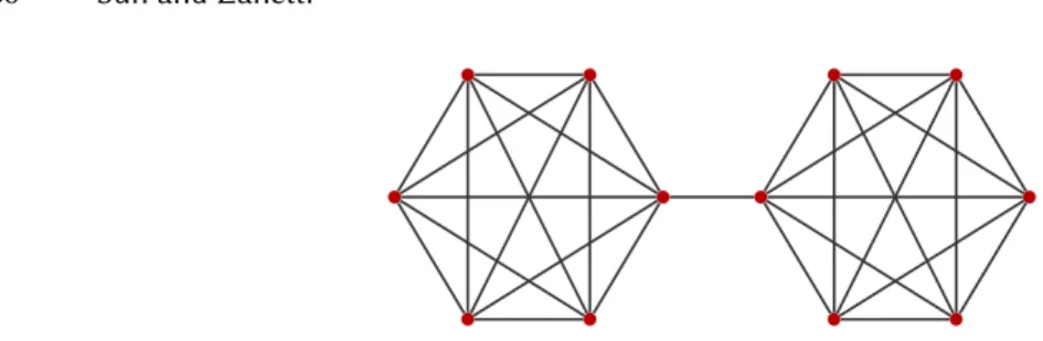
In this section we present an algorithm for constructing a cluster-preserving sparsifier that can be easily imple-mented in the distributed setting. Our algorithm is based on sampling edges with respect to the degrees of their endpoints, which was originally introduced in (Spielman and Teng 2011) as a way to construct spectral sparsifiers for graphs withhighspectral expansion. To sketch the intuition behind our algorithm, let us look at the following toy example illustrated in Figure1, i.e., the graphGconsisting of two complete graphs ofnnodes connected by a single edge. It is easy to see that, when we sampleO(nlogn)edges uniformly at random fromGto form a graph
H, with high probability the middle edge will not be sampled andH will consist of two isolated expander graphs, each of which has constant spectral expansion. Although our sampled graphHdoes not preserve the spectral and cut structure ofG, it does preserve its cluster-structure: every reasonable clustering algorithm will recover these two disjoint components ofH, which correspond exactly to the two clusters inG. We will show that this sampling scheme can be generalised, and sampling every edgee={u,v}with probability depending only ondu anddvsuffices to construct a sparse subgraph that preserves the cluster-structure of the original graph.
3.1 Algorithm description
In our algorithm every nodeu checks every edgee = {u,v} adjacent tou itself, and samples edgee with probability pu(v),min w(u,v) · C·logn du·λk+1 ,1 (3)
for a large enough constantC ∈R>0. The algorithm uses a setFto maintain all the sampled edges, whereF is initially set to be empty. Finally, the algorithm returns a weighted graphH =(V,F,wH), where the weight ACM Transactions on Parallel Computing, Vol. x, No. 4, Article 00. Publication date: March 201x.
1 2 3 4 5 6 7 8 9 10 11 12 13 14 15 16 17 18 19 20 21 22 23 24 25 26 27 28 29 30 31 32 33 34 35 36 37 38 39 40 41 42 43 44 45 46 47 48 1 2 3 4 3 4 1 2 3 4 3 4
Fig. 1. The graphGconsists of two complete subgraphs ofnnodes connected by an edge. It is easy to see that sampling
O(nlogn)edges uniformly at random suffices to construct a subgraph having the same cluster-structure ofG.
wH(u,v)of every sampled edgee={u,v} ∈F is defined as
wH(u,v), w(u,v)
pe ,
and
pe ,pu(v)+pv(u) −pu(v) ·pv(u)
is the probability thate ={u,v}is sampled by at least one of its endpoints. Notice that our algorithm can be easily implemented in a distributed setting: any nodeuchooses to retain (or not) an edgeu∼vindependently from any other node, and communication betweenuandvis needed only ifu∼vis sampled by one of its two endpoints. Therefore, the total communication cost of the algorithm is linear in the number of edges inH.
3.2 Analysis of the algorithm
Now we analyse the algorithm, and prove Theorem1.1. At a high level, our proof consists of the following two steps:
(1) We show that the conductance ofS1, . . . ,Skare approximated preserved inH, i.e.,
ϕH(Si)=O(k·ϕG(Si)) for anyi=1, . . . ,k. (4) (2) We analyse the intra-connectivity of the clusters in the returned graphH, and prove that the topn−k
eigenspaces ofLGare preserved inLH. This implies thatλk+1(LH)=Ω(λk+1(LG)).
Combining these two steps, we will prove thatϒH(k)=Ω(ϒG(k)/k), which proves the approximation guarantees of Theorem1.1. The total number of edges inH follows by the sampling scheme of our algorithm. We first recall the following concentration inequalities that will be used in our proof.
Lemma 3.1 (Bernstein’s ineqality (Chung and Lu 2006)). LetX1, . . . ,Xn be independent random variables such that|Xi|6Mfor anyi ∈ {1, . . . ,n}. LetX =Íni
=1Xi and letR= Ín
i=1E[X 2
i]. Then, it holds that
P[ |X−E[X]|>t]62exp − t 2 2(R+Mt/3) .
Lemma 3.2 (Matrix Chernoff Bound, (Tropp 2012)). Consider a finite sequence{Xi}of independent, random, PSD matrices of dimensiondthat satisfykXik 6R. Letµmin ,λmin(E[
Í
iXi])andµmax,λmax(E[ Í
1 2 3 4 5 6 7 8 9 10 11 12 13 14 15 16 17 18 19 20 21 22 23 24 25 26 27 28 29 30 31 32 33 34 35 36 37 38 39 40 41 42 43 44 45 46 47 48 it holds that P " λmin Õ i Xi ! 6(1−δ)µmin # 6d· e−δ (1−δ)1−δ µmin/R forδ∈ [0,1], and P " λmax Õ i Xi ! >(1+δ)µmax # 6d· eδ (1+δ)1+δ µmax/R forδ >0. Proof of Theorem1.1. We first analyse the size ofF. Since
Õ u∈V Õ e={u,v} w(u,v) · Clogn du·λk+1 =O nlogn λk+1 ,
it holds by Markov inequality that the number of edgese ={u,v}withpu(v)>1 isO((1/λk+1) ·nlogn). Without loss of generality, we assume that these edges are inF, and in the remaining part of the proof we assume it holds for any edgeu∼vthat
w(u,v) · C·logn du ·λk+1
<1. Then, the expected number of edges inH equals to
Õ e={u,v} pe 6 Õ e={u,v} pu(v)+pv(u)= Õ e={u,v} w(u,v) · C·logn du·λk+1 +w(u,v) · C·logn dv·λk+1 =O nlogn λk+1 , and by Markov inequality it holds with constant probability that|F|=O((1/λk+1) ·nlogn). This implies that the total information exchanged among all nodes is|F|=O((1/λk+1) ·nlogn). TheO(1)rounds needed for the algorithm is simply by the algorithm description.
Now we will show that the degrees of nodes inH are approximately preserved with high probability. Letube an arbitrary node ofG. For any edgee ={u,v}, we define random variableYeby
Ye = (w(u,v)
pe with probabilitype,
0 otherwise.
We further defineZu =Íe={u,v}Ye. Hence, it holds that E[Zu]= Õ e={u,v} E[Ye]= Õ e={u,v} pe·w(u,v) pe = Õ e={u,v} w(u,v)=du. For the second moment, we have that
Ru , Õ e={u,v} EY2 e= Õ e={u,v} pe· w(u,v) pe 2 = Õ e={u,v} (w(u,v))2 pe . (5)
Sincepe =pu(v)+pv(u) −pu(v)pv(u)>pu(v), we can rewrite (5) as
Ru = Õ e={u,v} E[Y2 e]6 Õ e={u,v} (w(u,v))2 pu(v) = Õ e={u,v} (w(u,v))2 ·du ·λk+1 w(u,v) ·C·logn = d2 u·λk+1 C·logn. On the other hand, we have for anye={u,v}that
06 w (u,v) pe 6 w(u,v) pu(v) = du ·λk+1 C·logn,
1 2 3 4 5 6 7 8 9 10 11 12 13 14 15 16 17 18 19 20 21 22 23 24 25 26 27 28 29 30 31 32 33 34 35 36 37 38 39 40 41 42 43 44 45 46 47 48
by applying Bernstein’s inequality (Lemma3.1) we have that
P |dH(u) −du| > 1 2 ·du =P |Zu−E[Zu]|> 1 2 ·E[Zu] 62·exp© « − d 2 u/8 d2 u·λk+1 Clogn + 1 6· d2 uλk+1 Clogn ª ® ¬ =2·exp − Clogn/8 λk+1+λk+1/6 =o(1/n).
Hence, it holds by the union bound that, with high probability, the degree of all the nodes inHare approximately preserved up to a constant factor. We assume that this event occurs in the rest of the proof. This implies that volH(S)=Θ(volG(S))for any subsetS ⊆V.
We continue to show thatϕH(Si)=O(k·ϕG(Si))for any 16i 6k, whereS1, . . . ,Skform an optimal clustering inG. By the definition ofYe, it holds for any 16i 6kthat
E[wH(Si,V\Si) ]=E Õ e={u,v}, u∈Si,v<Si Ye = Õ e={u,v}, u∈Si,v<Si pe·w(u,v) pe =w(Si,V \Si).
Hence, by Markov’s inequality and the union bound, with constant probability it holds for alli=1, . . . ,kthat
wH(Si,V\Si)=O(k·w(Si,V \Si)), (6)
i.e., the cut value betweenSi andV\Si is approximately preserved for any 16i6k. Therefore, it holds with constant probability that
ρH(k)6 max 16i6k
ϕH(Si)= max 16i6k
O(k·ϕG(Si))=O(k·ρG(k)).
Secondly, we show that the cluster-structure ofGis approximately preserved inH. LetLGbe the projection ofLG on its topn−keigenspaces, andLGcan be written as
LG = n Õ i=k+1 λifif| i .
With a slight abuse of notation we callL
−1/2
G the square root of the pseudoinverse ofLG, i.e.,
LG−1/2= n Õ i=k+1 (λi)−1/2 fif| i .
Analogously, we callIthe projection on span{fk+1, . . . ,fn}, i.e.,
I= n Õ i=k+1 fif| i .
We will prove that the topn−k eigenspaces ofLGare preserved, which implies thatλk+1(LG)=Θ(λk+1(LH)). To prove this, we recall that the probability that every edgee={u,v}is sampled inH is
1 2 3 4 5 6 7 8 9 10 11 12 13 14 15 16 17 18 19 20 21 22 23 24 25 26 27 28 29 30 31 32 33 34 35 36 37 38 39 40 41 42 43 44 45 46 47 48
and it holds that1
2(pu(v)+pv(u))6pe 6pu(v)+pv(u). Now for each edgee={u,v}ofGwe define a random matrixXe ∈Rn×nby Xe= ( wH(u,v) · L−1/2 G bebe|L −1/2
G ife ={u,v}is sampled by the algorithm,
0 otherwise,
where we recall thatbe =χu−χvfor edgee={u,v}. Notice that Õ e∈E[G] Xe = Õ sampled edgese={u,v} wH(u,v) · L−1/2 G bebe|L −1/2 G =L −1/2 G LH0L −1/2 G , where LH0 = Õ sampled edgese={u,v} wH(u,v) ·beb| e
is essentially the Laplacian matrix ofHbut is normalised with respect to the degrees of the nodes in the original graphG, i.e.,LH0 =DG−1DH−D−
1/2
G AHD −1/2
G . We will prove that, with high probability, the topn−keigenspaces ofLH0 andLGare approximately the same. Later we will show the same holds forLHandL0H, which implies thatλk+1(L
0
H)=Ω(λk+1(LG)).
We start looking at the first moment of the expression above:
E " Õ e∈E Xe # = Õ e={u,v} ∈E[G] pe·wH(u,v) · LG−1/2bebe|L−G1/2 = Õ e={u,v} ∈E[G] pe·w(u,v) pe · L −1/2 G bebe|L −1/2 G =LG−1/2LGLG−1/2=I.
Moreover, for any samplede={u,v} ∈Ewe have that
kXek6wH(u,v) ·be|LG−1/2L−G1/2be=w(u,v) pe ·be|L −1 Gbe 6w(u ,v) pe · 1 λk+1 · kbek2 6 2λk+1 C·logn· 1 du + 1 dv · 1 λk+1 1 du + 1 dv 6C 2 logn,
where the second inequality follows by the min-max theorem of eigenvalues. Now we apply the matrix Chernoff bound (Lemma3.2) to analyse the eigenvalues ofÍe∈EXe, and build a connection between λk+1(L0
H)and
λk+1(LG). By setting the parameters of Lemma3.2by µmax = λmax E Í
e∈E[G]Xe = λmax
I = 1,R = 2/(C·logn)andδ =1/2, we have that
P λmax© « Õ e∈E[G] Xeª ® ¬ >3/2 6n· e1/2 (1+1/2)3/2 Clogn/2 =O(1/nc) for some constantc. This gives us that
P λmax© « Õ e∈E[G] Xeª ® ¬ 63/2 =1−O(1/nc). (7) ACM Transactions on Parallel Computing, Vol. x, No. 4, Article 00. Publication date: March 201x.
1 2 3 4 5 6 7 8 9 10 11 12 13 14 15 16 17 18 19 20 21 22 23 24 25 26 27 28 29 30 31 32 33 34 35 36 37 38 39 40 41 42 43 44 45 46 47 48
On the other side, since our goal is to analyseλk+1(L0
H)with respect toλk+1(LG), it suffices to work with the top(n−k)eigenspace ofLG. SinceE[Íe∈EXe]=I, we can assume without loss of generality thatµmin=1.
1
Hence, by settingR=2/(C·logn)andδ =1/2, we have that P λmin© « Õ e∈E[G] Xeª ® ¬ 61/2 =n· e−1/2 (1/2)1/2 Clogn/2 =O(1/nc) for some constantc. This gives us that
P λmin© « Õ e∈E[G] Xeª ® ¬ >1/2 =1−O(1/nc). (8) Combining (7), (8), and the fact ofÍe∈E[G]Xe =L
−1/2
G LH0 L −1/2
G , with probability 1−O(1/nc)it holds for any non-zerox ∈Rn in the space spanned byfk+1, . . . ,fnthat
x|L−1/2 G LH0 L −1/2 G x x|x ∈ (1/2,3/2). (9) By settingy=L −1/2 G x, we can rewrite (9) as y|L0 Hy y|L1G/2L1G/2y =y|L 0 Hy y|LGy = y|L0 Hy y|y y|y y|LGy ∈ ( 1/2,3/2).
Since dim(span{fk+1, . . . ,fn})=n−k, we have just proved there existn−korthogonal vectors whose Rayleigh quotient with respect toL0
H isΩ(λk+1(LG)). By the Courant-Fischer Theorem, we have
λk+1(L 0 H)> 1 2λk+ 1(LG). (10)
It remains to show thatλk+1(LH)=Ω λk+1(L
0
H), which implies thatλk+1(LH)=Ω(λk+1(LG))by (10). By the definition ofL0 H, we have thatLH =D−1/2 H D 1/2 G LH0D 1/2 G D −1/2
H . Therefore, for anyx ∈Rnandy=D1/2
G D −1/2 H x, it holds that x|LHx x|x = y|L0 Hy x|x > 1 2 ·y |L0 Hy y|y , (11)
where the last equality follows from the fact that the degrees inH andGdiffer just by a constant multiplicative factor, and therefore,
y|y=D1/2 G D −1/2 H x | D1/2 G D −1/2 H x =x|D GD−H1x > 1 2 ·x|x.
Finally, we show that (11) implies thatλk+1(LH) >(1/2) ·λk+1(L
0
H). To see this, letS1 ⊆Rn be a(k+1)-th dimensional subspace ofRn such that
λk+1(LH)=max x∈S1 x|LHx x|x . LetS2= n D1/2 G D −1/2 H x:x ∈S1 o
. Notice that sinceD1/2
G D−1/2is full rank,S2has dimensionk+1. Therefore,
λk+1(L 0 H)= min S: dim(S)=k+1 max y∈S y|L0 Hy y|y 6maxy∈S2 y|L0 Hy y|y 62 maxx∈S1 x|LHx x|x =2λk+1(LH), (12) 1
To understand why this is the case, notice we could have definedXeas an(n−k)-dimensional operator. Then,Iwould be just the identity in this(n−k)-dimensional space.
1 2 3 4 5 6 7 8 9 10 11 12 13 14 15 16 17 18 19 20 21 22 23 24 25 26 27 28 29 30 31 32 33 34 35 36 37 38 39 40 41 42 43 44 45 46 47 48
where the last inequality follows by (11). Combining (10) with (12) gives us thatλk+1(LH)=Ω(λk+1(G)), which
impliesϒH(k)=Ω(ϒG(k)/k).
4 DISTRIBUTED GRAPH CLUSTERING
In this section we present and analyse a distributed algorithm to partition a graphGthat possesses a cluster-structure with clusters of balanced size, and prove Theorem1.2. Throughout the section, we assume thatS1, . . . ,Sk are the optimal clusters satisfying vol(Si)>βvol(V)for any 16i6k.
4.1 Algorithm description
Our algorithm consists of Seeding, Averaging, and Query steps, which are described as follows. The Seeding step:The algorithm sets
¯ s=Θ1 β ·log 1 β ,
and each nodevchooses to beactivewith probability ¯s·dv/vol(V). For simplicity, we assume thatv1,· · ·,vs are the active nodes, for somes ∈N. The algorithm associates each active node with a vectorx(0,i)=χv
i, and these vectorsx(0,1), . . . ,x(0,s)represent the initial state (round 0) of the graph, where each nodevonly maintains the valuesx(0,1)(v), . . . ,x(0,s)(v). Notice that the information about which nodes are active doesn’t need to be broadcasted during the seeding step of the algorithm.
The Averaging step:This step consists ofT rounds, and in each round every nodevupdates its state based on the states of its neighbours from the previous round. Namely, for any 16i 6s, the valuesx(t,i)(v)maintained by nodevin roundtare computed according to
x(t,i)(v)= 1 2x (t−1,i) (v)+1 2 Õ {u,v} ∈E w(u,v) √ dudvx (t−1,i) (u). (13)
The Query step:Every nodevcomputes the label`vof the cluster that it belongs to by the formula `v =min i | x(T,i)(v)> √ dv 2βvol(V) . (14)
Notice that the execution of the algorithm requires each node to know certain parameters about the graph, including the number of nodesn, the volume of the graph vol(V), a boundβon the size of the clusters, and the value ofT. However, nodes do not need to know the exact values of these parameters, but only a reasonable approximation. Moreover, although the value ofT is application-dependent, for graphs with clusters that have strong intra-connectivity properties, we can setT ≈lognin practice.
4.2 Analysis of the algorithm
In this subsection we analyse the distributed clustering algorithm, and prove Theorem1.2. Recall that we assume
Ghas an optimal clusteringS1, . . . ,Sk with vol(Si)>βvol(V)for any 16i 6k, andGsatisfies the following gap assumption: ϒG(k)=ω k2 log2 1 β +logn . (15)
Before analysing the algorithm, we first describe some intuitions behind the proof. We usex(t,1), . . . ,x(t,s)to denote the configuration of the algorithm’s execution in roundt, and these vectors are updated according to (13). For the sake of intuition, we assume thatGis regular, and the vectorx(t,i)corresponds to the probability distribution of at-step lazy random walk inG. It is well-known that, after a sufficient number of rounds, the vectorsx(t,i)s are close to the uniform distribution, which would provide no information about the structure ACM Transactions on Parallel Computing, Vol. x, No. 4, Article 00. Publication date: March 201x.
1 2 3 4 5 6 7 8 9 10 11 12 13 14 15 16 17 18 19 20 21 22 23 24 25 26 27 28 29 30 31 32 33 34 35 36 37 38 39 40 41 42 43 44 45 46 47 48
of clusters in a graph. However, the timeT =Θ(logn/λk+1)can be informally viewed as thelocal mixing time of some clusterSi: when a random walk starts with somev ∈Si and the random walk does not leaveSi, the resulting distribution of thisT-step random walk will be close to the uniform one supported on the node set ofSi. We will formalise the fact by showing that, when picking a starting vertex uniformly at random fromSi, with high probability the probability mass of aT-step random walk will be concentrated onSi. In other words, afterT rounds, each vectorx(T,1), . . . ,x(T,s)is almost uniform on one of the clusters, and close to zero everywhere else. This further implies that, once the algorithm ensures that there is at least one active node from every cluster, the query step will assign the same label to two nodes if and only if they belong to the same cluster. WhenGis not regular, the averaging step defined in (13) can be viewed as apower iteration methodto approximate (klinearly independent combination of ) the bottom eigenvectors ofLG. We will show that these eigenvectors contain all the information needed to obtain a good partitioning of the graph.
We first analyse the properties of aT-stepsinglerandom walk, and letx(i)be the distribution that the random walk reaches a specific vertex afteristeps. Let
I= k Õ i=1 fif| i
be the projection on the bottomkeigenspaces. The following lemma shows that, whenx(0)is the initial distribution of a random walk, afterT steps the distributionx(T)that the random walk reaches a specific node is close to
Ix(0).
Lemma 4.1. For a large constantc>0, it holds x (T)− Ix(0) =O logn ϒG(k)· Ix (0) +n −c.
Proof. We introduce the matrixPdefined by P=1 2 ·I+1 2 ·D−1/2 AD−1/2 =I−1 2 LG.
Hence, by the description of the averaging step, it holds thatx(t)=Px(t−1), which implies thatx(T)=PTx(0). To analyse the property ofx(T), we study the spectral property ofPT, which can be written as
PT = I−1 2 LG T = n Õ i=1 1−λi 2 T fif| i = k Õ i=1 1−λi 2 T fif| i + n Õ i=k+1 1−λi 2 T fif| i , (16)
where we recall thatλ1 6. . .6λnare the eigenvalues ofLGwith the corresponding eigenvectors f1, . . . ,fn. We look at the second term in (16) and, by settingT =clogn/λk+1, it holds fori >k+1 that
1−λi 2 T 6 1−λk+1 2 2c·logn/λk+1 6e−clogn 6n−c, (17)
where the second inequality holds by the fact thatλk+1/261 and 1−x 6e−xholds forx∈ [−1,1]. Similarly, we look at the first term in (16) and it holds for any 16i 6kthat
1−λi 2 T >1−T ·λi 2 = 1−O λi ·logn λk+1 =1−O logn·λk λk+1 , (18)
1 2 3 4 5 6 7 8 9 10 11 12 13 14 15 16 17 18 19 20 21 22 23 24 25 26 27 28 29 30 31 32 33 34 35 36 37 38 39 40 41 42 43 44 45 46 47 48
where the first inequality holds by the fact that(1+x)r >1+rxfor anyx >−1 andr >1. Combining (16), (17) and (18), we upper bound the distance betweenx(T)andIx(0)by
x (T)− Ix(0) 2 = PT − Ix(0) 2 = k Õ i=1 1− 1−λi 2 T! fif| i x( 0)+ n Õ i=k+1 1−λi 2 T fif| i x( 0) 2 = k Õ i=1 1− 1−λi 2 T!2 D fi,x(0)E 2 + n Õ i=k+1 1−λi 2 2T D fi,x(0)E 2 =O logn·λk λk+1 2 k Õ i=1 D fi,x(0)E 2 +n−2c ! =O logn·λk λk+1 · Ix (0) 2 +n−2c ! =O logn ϒG(k)· Ix (0) 2 +n−2c ! , where the last inequality uses the fact that
λk λk+1 6 ρ(k) 2λk+1 = 1 2ϒG(k)
by the higher-order Cheeger inequality (Lee et al. 2014). Then, taking the square root on both sides of the equality
above proves the lemma.
Our algorithm is to recover the structure of clusters based onx(T), and the previous lemma builds a connection betweenx(T)andI. Next, we will build a connection betweenIand the indicator vectors ofS1, . . . ,Sk. Based on Lemma4.2, we will prove in Lemma4.3that the bottomkeigenvectors ofLGare close to a linear combination of the indicator vectors ofS1, . . . ,Sk, which implies the structure of clusters can be approximately recovered from
x(T).
Lemma 4.2 ((Peng et al. 2015)). Let{Si}k
i=1be ak-way partition ofGachievingρ(k), and letϒG(k)=Ω k 2
. Assume thateχi is the projection offi in the span of{χS1, . . . ,χSk}. Then, it holds for any16i6kthat
keχi −fik=O s k ϒG(k) ! . Lemma 4.3. LetϒG(k)=Ω k2. For any16i6kthere exists
b χi ∈span{χS 1, . . . ,χSk}such that kbχi −fik=O s k ϒG(k) ! . Moreover,{bχi}ki=1form an orthonormal set.
Proof. Since{fi}k
i=1is an orthonormal set, it holds by Lemma4.2that{eχi}
k
i=1arealmostorthonormal. Hence, our task is to construct an orthonormal set{
b
χi}ki=1based on{eχi}
k
i=1, which can be achieved by applying the ACM Transactions on Parallel Computing, Vol. x, No. 4, Article 00. Publication date: March 201x.
1 2 3 4 5 6 7 8 9 10 11 12 13 14 15 16 17 18 19 20 21 22 23 24 25 26 27 28 29 30 31 32 33 34 35 36 37 38 39 40 41 42 43 44 45 46 47 48
Gram-Schmidt orthonormalisation procedure. We start by setting
b χ1 , e χ1 keχ1k . By Lemma4.2and the triangle inequality, it holds that
| keχ1k −1|=| keχ1k − kf1k | 6keχ1−f1k=O s k ϒG(k) ! , which implies that
kbχ1−eχ1k= e χ1 keχ1k −eχ1 = 1 keχ1k −1 · keχ1k=| keχ1k −1|=O s k ϒG(k) ! . By another application of the triangle inequality, this implies that
kbχ1−f1k6kbχ1−eχ1k+keχ1−f1k=O s k ϒG(k) ! .
For any 26i 6k, we inductively construct b
χi in the following way:
b χi , eχi − Íi−1 j=1heχi,bχjibχj eχi −Íi −1 j=1heχi,bχjibχj . By construction,{ b
χi}ki=1are orthonormal. It remains to boundkbχi−fik. Notice that eachbχi is a linear com-bination of
e
χ1, . . . ,eχi. Indeed,{bχ1, . . . ,bχi−1}is a basis of the space spanned byeχ1, . . . ,eχi−1. LetQi−1be the orthogonal projection of the space spanned by
e
χ1, . . . ,eχi−1. We have that e χi− i−1 Õ j=1 heχi,bχjibχj −fi
=keχi−Qi−1eχi −fik6keχi−fik+kQi−1eχik. (19)
By Lemma4.2we know thatk e
χi −fik=OqϒGk(k). Moreover, it holds that
kQi−1eχik=keχik − k(I−Qi−1)eχik61− keχi−fik − |heχi,fii|=O s
k
ϒG(k)
!
, (20)
where the last equality follows again by Lemma4.2. Combining with (19) and (20), we have that
e χi − i−1 Õ j=1 heχi,bχjibχj−fi =O s k ϒG(k) ! . (21)
1 2 3 4 5 6 7 8 9 10 11 12 13 14 15 16 17 18 19 20 21 22 23 24 25 26 27 28 29 30 31 32 33 34 35 36 37 38 39 40 41 42 43 44 45 46 47 48
This implies that
kbχi −fik= e χi −Íi−1 j=1heχi,bχjibχj eχi −Íi− 1 j=1heχi,bχjibχj −fi 6 e χi−Íi−1 j=1heχi,bχjibχj eχi−Íi− 1 j=1heχi,bχjibχj − eχi − i−1 Õ j=1 heχi,bχjibχj ! + e χi− i−1 Õ j=1 heχi,bχjibχj ! −fi = 1 eχi −Íi− 1 j=1heχi,bχjibχj −1 · e χi− i−1 Õ j=1 heχi,bχjibχj +O s k ϒG(k) ! = e χi − i−1 Õ j=1 heχi,bχjibχj −1 +O s k ϒG(k) ! = e χi − i−1 Õ j=1 heχi,bχjibχj − kfik +O s k ϒG(k) ! 6 e χi− i−1 Õ j=1 heχi,bχjibχj−fi +O s k ϒG(k) ! =O s k ϒG(k) ! ,
where the third line follows from (21), the sixth line follows from the triangle inequality, and the last line follows
from (21).
Based on Lemma4.3, we will prove that there is a setAconsisting of a sufficient number of “good” nodes such that, for any random walk starting fromv ∈A∩Sj for some 16j 6k, the resulting distribution of aT-step random walk fromvis close to the indicator vector ofSj. This fact is formalised as follows:
Lemma 4.4. There is a setA⊆V with
vol(A)>vol(V)
1− β
Clog(1/β)
for some constantCsuch that, for anyj=1, . . . ,kand anyv∈A∩Sj, settingx(0)=χvwe have that x(T) −p 1 vol(Sj) χSj =O logn ϒG(k) ·pβvol(V) + s k2 log(1/β) ϒG(k)βvol(V) ! . Proof. Without loss of generality we assumev∈Sj, and let{
b
χi}ki=1be the set of vectors defined in Lemma4.3. We show that the projection ofχvon span{
b
χ1, . . . ,bχk}is exactly equal to 1
√
vol(Sj)χSj
. To this end, first notice
that span{ b
χ1, . . . ,bχk} =span{χS1, . . . ,χSk}, since each bχi is by definition a linear combination of vectors in
{χSi}ki=1and dim(span{ b χ1, . . . ,bχk})=dim span{χS1, . . . ,χSk} =k. Then, k Õ i=1 hχv,bχiibχi = k Õ i=1 χv,χSi χSi = χv,χSj χSj = 1 p vol(Sj) χSj. (22)
1 2 3 4 5 6 7 8 9 10 11 12 13 14 15 16 17 18 19 20 21 22 23 24 25 26 27 28 29 30 31 32 33 34 35 36 37 38 39 40 41 42 43 44 45 46 47 48
where the first equality holds by the fact that span{ b
χ1, . . . ,bχk}=span{χS1, . . . ,χSk}and the orthonormality of
the two sets of vectors, and the second holds becauseχvis orthogonal to everyχS
`with`,j.
Now we start with analysing the distance between the resulting distribution of aT-step random walk starting withv ∈Sjand √ 1
vol(Sj)χSj
. First of all, we apply the triangle inequality and have that
x(T)− 1 p vol(Sj) χSj 6 x (T)− Iχv + Iχv−p 1 vol(Sj) χSj . (23)
We will analyse the two terms in the right hand size of (23) separately. By Lemma4.1we have
x (T)− Iχv =O logn·Iχv ϒG(k) +n −c ! . (24)
To show that the term above is small, we introduce for anyv ∈V a parameterαvwhich represents how far the b
χi’s are from the bottom eigenvectors in the entries corresponding tov, i.e.,
αv , v u t 1 dv k Õ i=1 (fi(v) −bχi(v))2 , and we will prove that
Iχv =O 1 p vol(Sj) +αv ! . (25)
By expandingIχvas a linear combination off1, . . . ,fkwe have that
Iχv 2 = k Õ i=1 hχv,fii2 = k Õ i=1 hχv,bχi − (bχi−fi)i2 = k Õ i=1 (hχv,bχii − hχv,bχi −fii)2 6 k Õ i=1 2 hχv,bχii2 +hχv,bχi −fii2 (26) = 2 vol(Sj) + 2 k Õ i=1 hχv,bχi−fii2 (27) 6 2 vol(Sj)+ 2αv2 (28)
where (26) follows from the inequality(a−b)2 62(a2+b2), (27) follows from (22), and (28) follows from the definition ofαv. Hence, (25) holds and the first termx(T)− Iχv
in the right hand side of (23) can be upper bounded by x (T) − Iχv =O logn ϒG(k) · 1 p vol(Sj) +αv ! +n−c ! . (29)
1 2 3 4 5 6 7 8 9 10 11 12 13 14 15 16 17 18 19 20 21 22 23 24 25 26 27 28 29 30 31 32 33 34 35 36 37 38 39 40 41 42 43 44 45 46 47 48
Now we look at the second term in the right hand side of (23): by (22) and the triangle inequality we have that Iχv−p 1 vol(Sj) χSj = k Õ i=1 hχv,fiifi− k Õ i=1 hχv,fiibχi+ k Õ i=1 hχv,fiibχi− k Õ i=1 hχv,bχiibχi 6 k Õ i=1 hχv,fiifi− k Õ i=1 hχv,fiibχi + k Õ i=1 hχv,fiibχi− k Õ i=1 hχv,bχiibχi . (30) Let’s now analyse the two terms in (30) separately. For the first term, it holds that
k Õ i=1 hχv,fiifi − k Õ i=1 hχv,fiibχi 6 k Õ i=1 |hχv,fii| kfi −bχik 6O s k ϒG(k) ! · k Õ i=1 |hχv,fii| 6O s k ϒG(k) ! · v u t k Õ i=1 |hχv,fii|2 ·√k =O© « s k2 ϒG(k) ª ® ¬ ·Iχv =O s k2 ϒG(k)βvol(V)+αv ! (31)
where the first inequality follows from the triangle inequality, the second by Lemma4.3, the third one follows by the Cauchy-Schwarz inequality, and the last inequality follows by (25). For the second term of (30), we have
k Õ i=1 (hχv,fii − hχv,bχii)bχi = k Õ i=1 1 √ dv (fi(v) −bχi(v))bχi = v u t k Õ i=1 1 dv(fi(v) −bχi(v)) 2 =αv, (32) where the second equality follows from the orthonormality of{
b
χi}i. Combining (23), (29), (30), (31) and (32), we have x(T)− 1 p vol(Sj) χSj =O logn ϒG(k)· 1 p vol(Sj) +αv ! +n−c ! +O s k2 ϒG(k)βvol(V)+αv ! +αv =O logn ϒG(k) ·pβvol(V) +n−c+ s k2 ϒG(k)βvol(V)+αv ! . (33)
Let’s define the set
B, ( v|αv > s Ck2 log(1/β) ϒG(k)βvol(V) ) , for some constantC. Let us look at vol(B)now. By Lemma4.3we know that
Õ v∈V dvα2 v= k Õ i=1 Õ v∈V (fi(v) −bχi(v))2 = k Õ i=1 kfi−bχik2 6 k 2 ϒG(k).
1 2 3 4 5 6 7 8 9 10 11 12 13 14 15 16 17 18 19 20 21 22 23 24 25 26 27 28 29 30 31 32 33 34 35 36 37 38 39 40 41 42 43 44 45 46 47 48
By the definition ofBand the averaging argument, it holds that vol(B)6 k 2 ϒG(k)· ϒG(k)βvol(V) Ck2log(1/β) = βvol(V) Clog(1/β). (34)
By (33) and the definition ofB, we have that for allv ∈Sj\B, by settingx(0)=χvwe have that x(T) −p 1 vol(Sj) χSj =O logn ϒG(k) ·pβvol(V) + s k2 ϒG(k)βvol(V)+ s Ck2 log(1/β) ϒG(k)βvol(V) ! =O logn ϒG(k) ·pβvol(V) + s k2log(1/β) ϒG(k)βvol(V) ! .
By definingA=V \B, we proved the statement.
So far we analysed the case of aT-step single random walk: we showed that there is a sufficient number of “good” nodes and, for anyT-step random walk starting from a good nodev ∈ Sj, inT steps the resulting distributionx(T)is close toχS
j. To identify all thekclusters simultaneously, our designed algorithm runs this process multiple times in parallel with carefully chosen initial nodes. In particular, as the resulting distribution
x(T)is close toχS
j for most random walks starting fromv∈ χSj, we need to ensure that there is a random walk starting with a good nodev∈Sj for any 16j 6k. This is why we introduce the Seeding step: by setting the probability ¯s·dv/vol(V)for every nodevto be active, it is easy to see that with constant probability there is at least an active node in each cluster.
Our analysis for the Query step is based on the relation between our averaging procedure and lazy random walks: since any single random walk gets well mixed inside a cluster afterT steps, we expect that the states of the nodes inside a cluster are similar. In particular, if theith random walk starts with a good node inSj, we expect thatx(T,i)(v) ≈1/vol(Sj)for mostv ∈Sjandx(T,i)(v) ≈0 otherwise. Hence, nodes from the same cluster will choose the same label based on (14), while nodes from different clusters will have different labels.
Proof of Theorem1.2. For each nodev, the probability that we start an averaging process with initial vector
χvis equal to ¯s·dv/vol(V), where ¯s=Θ
1
βlog1
β
. Hence, the probability that there exists ajsuch that no node fromSjis chosen as an initial node is at most
Ö v∈Sj 1− ¯ s·dv vol(V) 6 Ö v∈Sj e−s¯·dv/vol(V)=e− ¯ sÍ v∈Sjdv/vol(V) 6 1 200k,
where we used the inequality 1−x 6e−xforx 61, the assumption on the size of the clusters, i.e., vol(Sj)>
βvol(V), and the trivial fact thatβ 61/k. As a consequence, with probability greater than 199/200, for each clusterSj, at least one nodev∈Sj is chosen as a starting node of the averaging process.
Next, we bound the probability that all the starting nodes belong to the setAdefined in Lemma4.4. By the algorithm description, the actual number of active nodesssatisfiesE[s]=s¯. Therefore, it holds with probability 1−O(1)thats =O 1 βlog 1 β
. We assume that this event occurs in the rest of the proof. Letv1, . . . ,vs be the starting nodes. By Lemma4.4, the probability that there exists a starting nodevinot belonging toAis at most
P[there is some starting nodevi <A]6O( ¯
s) · (vol(V) −vol(A))
vol(V) 6 O(s) ·¯ β Clog(1/β) 6 1 200 .
Hence, with probability 1−O(1)every starting node belongs toA. For the rest of the proof we assume this is the case. For any nodev, letS(v)be the clustervbelongs to. Then, by the definition of the setA, it holds for any
1 2 3 4 5 6 7 8 9 10 11 12 13 14 15 16 17 18 19 20 21 22 23 24 25 26 27 28 29 30 31 32 33 34 35 36 37 38 39 40 41 42 43 44 45 46 47 48
starting nodevi that
x(T,i)− χS(vi) p vol(S(vi)) =O s k2log(1/β) ϒG(k)βvol(V) ! . (35)
On the other side, by the algorithm description we know that nodevcould be misclassified only if
x(T,i)(v)= x(T,i)(v) − χS(vi)(v) p vol(S(vi)) > √ dv 2βvol(V) for someisatisfyingS(vi),S(v), sinceχS(v
i)(v)=0 in this case. By studying a weaker condition we know that nodevcould be misclassified by the query step (14) only if there is someisuch that
x(T,i)(v) − χS(vi)(v) p vol(S(vi)) > √ dv 2βvol(V) , which is equivalent to x(T,i)(v) √ dv − χS(vi)(v) p dv·vol(S(vi)) 2 > 1 4β2vol(V)2. (36)
By (35) and the averaging argument the total volume of misclassified nodes is at most
O(s) ·¯ x(T,i)− 1 p vol(S(vi)) χS(vi) 2 ·4β2vol(V)2 =O 1 βlog 1 β · k2 ϒG(k) · log(1/β) βvol(V) + log2n ϒ2 G(k) ·βvol(V) ! ·β2 vol(V)2 ! =O k 2 ϒG(k)·log 2 1 β + log2n ϒ2 G(k) ·log 1 β ! vol(V).
Combining this with the assumption (15) proves the first statement. The second statement follows by the fact that the total communication among all nodes in each round isO(m· (1/β)log(1/β))words.
5 EXPERIMENTS
Now we present experimental results for our proposed algorithms. Since our clustering algorithm can be viewed as a distributed variant of the power method, we replace the distributed clustering algorithm by spectral clustering in order to evaluate our sparsification algorithm more accurately.
We test our sparsification algorithm on both synthetic and real-world datasets. To report a detailed and quantitative result, we will compare the clustering results of the following two approaches: (1) apply spectral clustering on the original input dataset; (2) apply spectral clustering on the graph returned by our sparsification algorithm. Besides giving the visualised results of our algorithm on various datasets, we use two functions to measure the quality of the above-mentioned two approaches: (1) For the synthetic datasets for which the underlying ground-truth clustering is known, the quality of a clustering algorithm is measured by the ratio of misclassified points, i.e.,
err(A1, . . . ,Ak), 1 n· k Õ i=1 |{v∈Ai :v <Si}|,
1 2 3 4 5 6 7 8 9 10 11 12 13 14 15 16 17 18 19 20 21 22 23 24 25 26 27 28 29 30 31 32 33 34 35 36 37 38 39 40 41 42 43 44 45 46 47 48
where {S1,· · ·,Sk} is the underlying ground-truth clustering and {A1, . . . ,Ak} is the one returned by the clustering algorithm. (2) For datasets for which a ground-truth clustering is not well-defined, the quality of a clustering is measured by thenormalised cut valuedefined by
ncut(A1, . . . ,Ak), k Õ i=1 w(Ai,V \Ai) vol(Ai) ,
which is a standard objective function for spectral clustering algorithms (Shi and Malik 2000;Von Luxburg 2007). All the experiments are conducted with Matlab and we use an implementation of the classical spectral clustering algorithm described in (Ng et al. 2001).
5.1 Datasets
We test the algorithms in the following three synthetic and real-world datasets, which are visualised in Figure2.
• Twomoons: this dataset consists ofnpoints inR2, wherenis chosen between 1,000 and 15,000. We consider each point to be a node. For any two nodesu,v, we add an edge with weightw(u,v)=exp(−ku−vk2/2σ2), whereσ =0.1.
• Gaussians: this dataset consists ofnpoints inR2, wherenis chosen between 1,000 and 15,000. Each point is sampled from a uniform mixture of 3 isotropic Gaussians of variance 0.04. The similarity graph is constructed in the same way asTwomoons, and we setσ =1 here.
• Sculpture: we use a 73×160 version of a photo ofThe Greek Slave2where each pixel is viewed as a node. To construct a similarity graph, we map each pixel to a point inR5with the form(x,y,r,д,b), where the last three coordinates are the RGB values. For any two nodesu,v, we put an edge betweenuandvwith weightw(u,v)=exp(−ku−vk2/2σ2), whereσ =20. This results in a graph with about 11,000 nodes andk=3 clusters.
These datasets are essentially the ones used in (Chen et al. 2016), which studies the effects of spectral sparsification on clustering. This makes it possible to easily compare our results with the state-of-the-art. The choice ofσvaries for different datasets, since they have in general different intra-cluster variance. There are several heuristics to choose the “correct” value ofσ(see, e.g., the classical reference (Ng et al. 2001)). In our case the value ofσ is chosen so that the spectral gap of the original similarity graph is large. This ensures that the clusters in the graph are well-defined, and spectral clustering outputs a meaningful clustering.
(a)Twomoons (b)Gaussians (c)Sculpture
Fig. 2. Visualisation of the datasets used in our experiments.
2
1 2 3 4 5 6 7 8 9 10 11 12 13 14 15 16 17 18 19 20 21 22 23 24 25 26 27 28 29 30 31 32 33 34 35 36 37 38 39 40 41 42 43 44 45 46 47 48
Table 1. Experimental results for theTwomoonsdataset, whereτ=C/λk+1is set to be0.8. Here err1and err2 stand for the
error ratios of spectral clustering on the original datasets and our sparsified graphs.
n # edges (%) err1 (%) err2 (%) 1,000 1.56 0.900 0.600 2,000 0.86 0.150 0.100 4,000 0.48 0.150 0.175 8,000 0.26 0.086 0.088 10,000 0.22 0.120 0.150 15,000 0.14 0.080 0.100
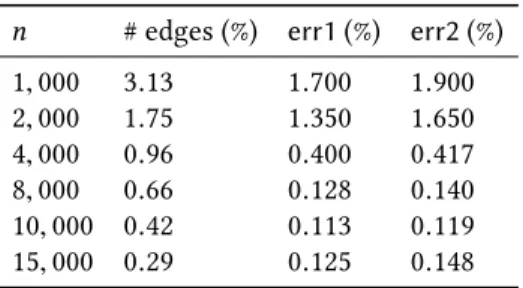
Table 2. Experimental results for theGaussiansdataset, whereτ=C/λk+1is set to be1.6. Here err1and err2 stand for the
error ratios of spectral clustering on the original datasets and our sparsified graphs.
n # edges (%) err1(%) err2(%) 1,000 3.13 1.700 1.900 2,000 1.75 1.350 1.650 4,000 0.96 0.400 0.417 8,000 0.66 0.128 0.140 10,000 0.42 0.113 0.119 15,000 0.29 0.125 0.148
5.2 Results on clustering quality
We test the performance of our algorithm on the three datasets. Notice that the sampling probability of the edges in our sparsification algorithm involves the factorC/λk+1. To find a desired value ofC/λk+1, denoted by
τ, we use the following doubling method: starting withτ =0.1, we double the value ofτ each time, until the spectral gap|λk+1−λk|of the resulting matrices doesn’t change significantly. Remarkably, for all the datasets considered in the paper,τ =1.6 always suffices for our purposes. Notice that this method will only increase the time complexity of our algorithm by at most a poly-logarithmic factor ofn.
For theTwomoonsandGaussiansdatasets, for all the tested graphs with size ranging from 1,000 to 15,000 points, our sparsified graphs require only about(1.63±1.5)% of the total edges. The error ratios of spectral clustering on the original datasets and our sparsified graphs are listed respectively aserr1 anderr2, and are always very close. See Table1and Table2for details.
TheSculpturedataset corresponds to a similarity graph ofn=11,680 nodes and 68 million edges. We run spectral clustering on both the input graph and our sparsified one, and compute the normalised cut values of each clustering in the original input graph. By settingτ =1.6, our algorithm samples only 0.37% of the edges (320,000) from the input graph. The normalised cut value of spectral clustering on the original dataset is 0.0938, while the normalised cut value of spectral clustering on our sparsified graph is 0.0935. The visualisations of the two clustering results are almost identical, as shown in Figure3.
ACKNOWLEDGMENTS
We would like to thank Dr. Emanuele Natale and Prof. Luca Trevisan who found a mistake in our paper that studies the same problem and appeared at SPAA’17. To fix that mistake, in the current paper we designed and
1 2 3 4 5 6 7 8 9 10 11 12 13 14 15 16 17 18 19 20 21 22 23 24 25 26 27 28 29 30 31 32 33 34 35 36 37 38 39 40 41 42 43 44 45 46 47 48
Fig. 3. Visualisation of the results onSculpture. The left-side picture is the original input dataset, the middle one is the
output of spectral clustering on the original input dataset, while the right-side picture is the output of spectral clustering on our sparsified graph.
analysed a different algorithm that works for a more general family of graphs. In particular, our algorithm works for non-regular graphs, while our claimed statement in the flawed SPAA’17 paper requires the underlying graph to be regular.
The second-named author wishes to acknowledge financial support received from the ERC Starting Grant (DYNAMIC MARCH).
REFERENCES
Zeyuan Allen-Zhu, Silvio Lattanzi, and Vahab S. Mirrokni. 2013. A Local Algorithm for Finding Well-Connected Clusters. In30th International
Conference on Machine Learning (ICML’13). 396–404.
Joshua Batson, Daniel A. Spielman, and Nikhil Srivastava. 2012. Twice-Ramanujan sparsifiers.SIAM J. Comput.41, 6 (2012), 1704–1721. Luca Becchetti, Andrea Clementi, Emanuele Natale, Francesco Pasquale, and Luca Trevisan. 2017. Find your place: Simple distributed
algorithms for community detection. In28th Annual ACM-SIAM Symposium on Discrete Algorithms (SODA’17). 940–959.
Luca Becchetti, Andrea E. F. Clementi, Pasin Manurangsi, Emanuele Natale, Francesco Pasquale, Prasad Raghavendra, and Luca Trevisan. 2018. Average Whenever You Meet: Opportunistic Protocols for Community Detection. In26th Annual European Symposium on Algorithms
(ESA’18). 7:1–7:13.
Andr ´as A. Bencz ´ur and David R. Karger. 1996. Approximatings-tminimum cuts inOe(n 2
)time. In28 Annual ACM Symposium on Theory of
Computing (STOC’96). 47–55.
Manuel Blum, Richard M. Karp, Oliver Vornberger, Christos H. Papadimitriou, and Mihalis Yannakakis. 1981. The Complexity of Testing Whether a Graph is a Superconcentrator.Inf. Process. Lett.13, 4/5 (1981), 164–167.
Jiecao Chen, He Sun, David P. Woodruff, and Qin Zhang. 2016. Communication-Optimal Distributed Clustering. In29th Advances in Neural
Information Processing Systems (NIPS’16). 3720–3728.
Fan Chung and Linyuan Lu. 2006. Concentration inequalities and martingale inequalities: a survey.Internet Math.3, 1 (2006), 79–127. Santo Fortunato. 2010. Community detection in graphs.Physics Reports486, 3 (2010), 75–174.
Shayan Oveis Gharan and Luca Trevisan. 2012. Approximating the Expansion Profile and Almost Optimal Local Graph Clustering. In53rd
Annual IEEE Symposium on Foundations of Computer Science (FOCS’12). 187–196.
Pan Hui, Eiko Yoneki, Shu Yan Chan, and Jon Crowcroft. 2007. Distributed community detection in delay tolerant networks. InProceedings of
2nd ACM/IEEE International Workshop on Mobility in the Evolving Internet Architecture.
David Kempe and Frank McSherry. 2004. A decentralized algorithm for spectral analysis. In36th Annual ACM Symposium on Theory of
Computing (STOC’04). 561–568.
James R. Lee, Shayan Oveis Gharan, and Luca Trevisan. 2014. Multiway Spectral Partitioning and Higher-Order Cheeger Inequalities.Journal
of the ACM61, 6 (2014), 37:1–37:30.
Yin Tat Lee and He Sun. 2015. Constructing Linear-Sized Spectral Sparsification in Almost-Linear Time. In56th Annual IEEE Symposium on
Foundations of Computer Science (FOCS’15). 250–269.
Yin Tat Lee and He Sun. 2017. An SDP-based algorithm for linear-sized spectral sparsification. In49th Annual ACM Symposium on Theory of
Computing (STOC’17).
Andrew Y. Ng, Michael I. Jordan, and Yair Weiss. 2001. On spectral clustering: Analysis and an algorithm. In14th Advances in Neural
1 2 3 4 5 6 7 8 9 10 11 12 13 14 15 16 17 18 19 20 21 22 23 24 25 26 27 28 29 30 31 32 33 34 35 36 37 38 39 40 41 42 43 44 45 46 47 48
Shayan Oveis Gharan and Luca Trevisan. 2014. Partitioning into Expanders. In25th Annual ACM-SIAM Symposium on Discrete Algorithms
(SODA’14). 1256–1266.
Richard Peng, He Sun, and Luca Zanetti. 2015. Partitioning Well-Clustered Graphs: Spectral Clustering Works!. In28th Conference on Learning
Theory (COLT’15). 1423–1455.
Jianbo Shi and Jitendra Malik. 2000. Normalized cuts and image segmentation.IEEE Transactions on pattern analysis and machine intelligence 22, 8 (2000), 888–905.
Daniel A. Spielman and Nikhil Srivastava. 2011. Graph Sparsification by Effective Resistances.SIAM J. Comput.40, 6 (2011), 1913–1926. Daniel A. Spielman and Shang-Hua Teng. 2013. A Local Clustering Algorithm for Massive Graphs and Its Application to Nearly Linear Time
Graph Partitioning.SIAM J. Comput.42, 1 (2013), 1–26.
Daniel A Spielman and Shang-Hua Teng. 2011. Spectral sparsification of graphs.SIAM J. Comput.40, 4 (2011), 981–1025.
Joel A. Tropp. 2012. User-friendly tail bounds for sums of random matrices.Foundations of computational mathematics12, 4 (2012), 389–434. Ulrike Von Luxburg. 2007. A tutorial on spectral clustering.Statistics and computing17, 4 (2007), 395–416.
Wenzhuo Yang and Huan Xu. 2015. A Divide and Conquer Framework for Distributed Graph Clustering. In32nd International Conference on
Machine Learning (ICML’15). 504–513.