Content-Based Scheduling of Virtual Machines
(VMs) in the Cloud
Sobir Bazarbayev
†, Matti Hiltunen
×, Kaustubh Joshi
×,
William H. Sanders
†, and Richard Schlichting
׆
University of Illinois at Urbana-Champaign,
×AT&T Labs Research
Abstract—Organizations of all sizes are shifting their IT infrastructures to the cloud because of its cost efficiency and convenience. Because of the on-demand nature of the Infras-tructure as a Service (IaaS) clouds, hundreds of thousands of virtual machines (VMs) may be deployed and terminated in a single large cloud data center each day. In this paper, we propose a content-based scheduling algorithm for the placement of VMs in data centers. We take advantage of the fact that it is possible to find identical disk blocks in different VM disk images with similar operating systems by scheduling VMs with high content similarity on the same hosts. That allows us to reduce the amount of data transferred when deploying a VM on a destination host. In this paper, we first present our study of content similarity between different VMs, based on a large set of VMs with different operating systems that represent the majority of popular operating systems in use today. Our analysis shows that content similarity between VMs with the same operating system and close version numbers (e.g., Ubuntu 12.04 vs. Ubuntu 11.10) can be as high as 60%. We also show that there is close to zero content similarity between VMs with different operating systems. Second, based on the above results, we designed a content-based scheduling algorithm that lowers the network traffic associated with transfer of VM disk images inside data centers. Our experimental results show that the amount of data transfer associated with deployment of VMs and transfer of virtual disk images can be lowered by more than 70%, resulting in significant savings in data center network utilization and congestion.
Index Terms—Scheduling, Virtualization, Data center, Cloud-computing.
I. INTRODUCTION
Today, large cloud service providers like Amazon Web Services (AWS), Rackspace, and Microsoft Azure have made it very cost-effective for companies to host their services on the cloud. Fast deployment and the pay-only-for-what-you-use nature of the cloud make it easy and convenient for companies to migrate applications and services to the cloud rather than own and maintain their own IT infrastructures. The rapid growth of cloud service providers can be seen in the size of their data centers. For example, according to [1], there are seven AWS data center locations around the world (four in the U.S.), and the total number of blade servers across all the locations is estimated at half a million.
The number of virtual machines (VMs) deployed in a large cloud data center each day can be very large, and their deployment introduces a significant load on the data center network. For example, we observed that an estimated
360,000 VMs were deployed in 24 hours in the East Coast data center of a major cloud provider (using the technique described in [2]). In typical data centers, VM disk images are stored in specialized storage racks and then transferred to compute nodes in other racks when a VM based on the image is deployed. The VM disk image sizes typically range from around 1 GB to tens of GBs. Transfer of such large numbers of such large VM disk images inside a data center introduces a significant amount of network traffic between racks. While the network architecture inside a data centers has been designed to accommodate such high network traffic, mainly through installation of expensive, specialized 10GbE switches between racks, it introduces a significant network cost and contention, for the limited network resources with application traffic to/from the VMs.
We propose a novel content-based VM scheduling algorithm that can significantly reduce the network traffic associated with transfer of VMs from storage racks to host racks in a cloud data center. Specifically, our algorithm takes advantage of the fact that different VM disk images share many common pages, especially if they use the same operating system and operating system version. While cloud providers typically provide a wide choice of VM images, and users can also bring their own VM images, the same operating systems and operating system versions are often used by different cloud users, resulting in many common pages. Furthermore, even though the contents of a VM disk change after the VM has been deployed and is in use, they still retain most of their similarity with the base image from which they were deployed. We used that characteristic of VMs to design our content-based scheduling algorithm. When deploying a VM, we search for potential hosts that have VMs that are similar in content to the VM being scheduled. Then, we select the host that has the VM with the highest number of disk blocks that are identical to ones in the VM being scheduled. Once we have chosen that host node, we calculate the difference between the new VM and the VMs residing at the host; then, we transfer only the difference to the destination host. Finally, at the destination host, we can reconstruct the new VM from the difference that was transferred and the contents of local VMs. Our experimental results show that this algorithm can result in a reduction of over 70% in the amount of data transfer associated with deployment of VM images. That saving is significant enough to have implications for data center network design and the
network congestion observed by VMs running on a cloud. While researchers have utilized the observation of identical pages in different VM images in the past to optimize VM deployment or live migration [3]–[6], our algorithm is to our knowledge the first one to utilize content similarity in VM disk images to optimize VM scheduling in a data center.
This paper is organized as follows. Section II presents related work and motivation. Section III presents design and technical details of our scheduling algorithm. In Section IV, we present our study and analysis of content similarity be-tween large sets of VM disk images we have collected. In Section V, we present a simulation of our scheduling algorithm in a data center and its results. Finally, we conclude in Section VII.
II. RELATEDWORK
An extensive evaluation of different sets of virtual machine disk images was done in [7] to test the effectiveness of deduplication for storing VM disk images. That paper shows promising results regarding content similarity among VM disk images.
A number of research projects have applied deduplication of identical pages among a group of related VMs being deployed [4] or migrated [5] from one source node to a specified destination node. However, our algorithm determines the node on which to deploy the new VM based on content similarity (scheduling), while those projects have taken the destination as given and did not consider scheduling. A special case of content similarity is considered in [6], which describes a process in which a VM is repeatedly migrated back and forth between two nodes. The pages of the migrated VM are stored at the original source node, and when the VM is migrated back to this node, only the pages that were modified need to be migrated back.
In the procedure described in [3], replicas of the VMs are stored in different nodes in order to speed up live migration of VMs. When a VM needs to be live-migrated, it is migrated to another node, where a replica of that VM is stored. In order to lower storage costs associated with storage of VM replicas, the authors use deduplication. Placement of VM replicas is based on content similarity between VMs; replicas are placed at nodes where storage savings can be maximized. Unlike our work, that project used content similarity to improve storage efficiency.
The fact that many VM instances share many common chunks or pages is utilized to speed up VM deployment and reduce the workload at the storage nodes in [8]. The strategy has compute nodes act as peers in a VDN (Virtual machine image Distribution Network), where a VM being deployed can be constructed from chunks being pulled from different compute nodes. However, [8] does not consider using content similarity in the scheduling decision.
A memory-sharing-aware placement of VMs in a data center was presented in [9]. Many data center virtualization solutions use content-based page sharing to consolidate the server’s
RAM resources. [10]–[12] studied maximization of page shar-ing in virtualized systems. In [9], runnshar-ing VMs with similar memory content are live-migrated to the same hosts. The costs associated with live-migration may diminish the benefits of memory-sharing in a data center. In our work, we saw that content-based scheduling of VMs leads to significant memory-sharing opportunities. VM disk images with high content similarity share many common libraries and applications. Our proposed content-based scheduling of VMs can lead to high memory sharing without live-migration of running VMs.
III. DESIGN
In this section, we first present background information on scheduling of VMs in data centers, and then describe design and implementation of our scheduling algorithm.
A. Background
In a typical Infrastructure as a Service (IaaS) deployment, a pool of VM disk images is stored in storage nodes. The images are templates for virtual machine file systems. VM instances are instantiated from these images at compute nodes. To deploy a VM instance, a user selects an image and instance type. An instance type typically specifies physical resources (such as CPU and RAM) that will be allocated for the instance once deployed. Once the user has specified the image he or she wants to deploy, a scheduling algorithm selects a compute node and copies the image from the storage node to the local storage of the compute node. Once copied, the VM can be booted up at the compute node.
The part of this process in which we are interested is the scheduling of VMs. The methods of VM scheduling algo-rithms used by major cloud service providers are proprietary. Hence, to explain VM scheduling in data centers, we will refer to the scheduling algorithm implemented in OpenStack [13]. OpenStack is open-source cloud software supported by thousands of developers, researchers, and the open-source community, in addition to hundreds of leading companies. The default scheduling implementation in OpenStack is the
filter scheduler, which consists of two phases: filtering and
weighting.
The task of thefiltering phase is to eliminate the compute nodes without sufficient resources (such as CPU and RAM) to host the new VM. The weighting phase assigns weights to the remaining compute nodes based on the states of the compute nodes and properties of the VM being scheduled. Its purpose is to select the most appropriate host for the VM being scheduled. For example, it would not be optimal to schedule a simple VM with low resource requirements on a high-performance host. The weights can incorporate load-balancing policies in the data center, utilization of nodes, and how well the available resources of the compute nodes match up with the VM resource requirements.
B. Scheduling Algorithm
Our scheduling algorithms were designed with the goal of lowering the amount of data transferred between racks in the
1: functionSELECTHOST(V MN)
2: Filter nodes based on available resources 3: Filter nodes ifV MNOS different from node OS 4: N←nrandomly selected nodes from filtered nodes 5: maxSimilarity=−1
6: fornode∈Ndo
7: forV M∈nodedo
8: similarity=calcSimilarity(V M, V MN) 9: ifsimilarity > maxSimilaritythen
10: maxSimilarity=similarity
11: selectedN ode=node
12: selectedN odeV M=V M
13: end if
14: end for
15: end for
16: return(selectedN ode, selectedN odeV M) 17: end function
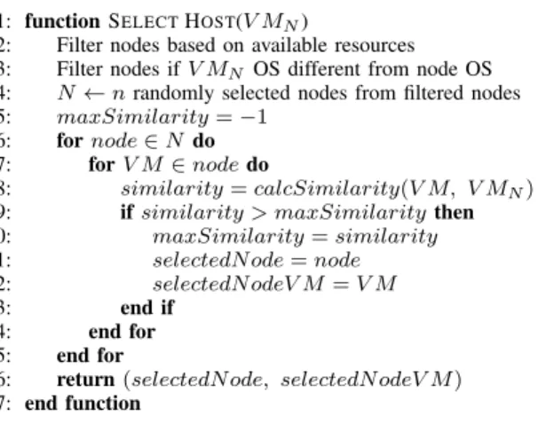
Fig. 1. Dedicated node scheduling algorithm.
data center when VM disk images are being copied to the host nodes. We achieved that goal through the colocation of VMs with high content similarity at the same hosts.
The architecture of our scheduler is as follows. There are management nodes that are separate from the compute and storage nodes in the data center that host the scheduler. Re-quests to deploy VMs are sent to the scheduler, which selects an appropriate compute node for each VM. The scheduler stores fingerprints for all of the virtual disk images from the image library. It also stores fingerprints for every running VM in the data center. For a running VM, the scheduler maintains a mapping between the VM’s fingerprint and the compute node hosting the VM. All the fingerprints are stored on the man-agement nodes. When VMs terminate, their fingerprints are removed from management nodes. Fingerprints are described in Section III-C1; they are used to estimate content similarity between two VM disk images.
We have designed two different content-based scheduling algorithms.
Dedicated nodes algorithm: In this algorithm, each compute
node is dedicated to hosting VMs with the same OS. For example, if a compute node is hosting a Ubuntu VM, then all the VMs hosted on the node will be Ubuntu VMs. We do not require the version numbers of the VMs to be the same on a compute node. Nodes get assigned specific OSs dynamically, as follows. When some VM with OSX is being scheduled,
if there are no nodes dedicated to OSX or if all the nodes
dedicated toOSX are full, then the VM is assigned to a node
that has no VMs running on it. As a result, that node becomes a dedicated node for OSX. When all the running VMs on a
certain node are terminated, that node is no longer dedicated to any OS.
In lines 2 and 3 in Figure 1, the scheduler eliminates the nodes that are not dedicated to the same OS as the new VM, and the nodes that do not have enough available resources to host the new VM. What remains are nodes that are dedicated to the new VM’s OS. Next, the scheduler selects n nodes randomly from the remaining nodes. In Section V, we will discuss how the different values of n affect the performance of the algorithm. The reason for randomly selecting the nodes
1: functionGENERATEFINGERPRINT(diskImage) 2: f ingerprint←bitArray(m)
3: f ingerprint.setAll(0)
4: hf1, . . . , hfk←kdifferent hash functions
5: whileblock=diskImage.read(4096)do
6: fori= 1→kdo
7: arrayIndex=hfi(block) %m
8: f ingerprint[arrayIndex] = 1 9: end for
10: end while
11: returnf ingerprint
12: end function
Fig. 2. Fingerprint generation for VM disk images.
is to balance the load in the data center. Then, the scheduler does content comparison between the new VM and all the running VMs at thenselected nodes (lines 5–15 in Figure 1). The new VM is assigned to the node hosting the VM with the highest content similarity to the new VM. The algorithm returns the selected node and the VM on that node with the highest content similarity, and that VM is used during transfer of the new VM to that node.
Greedy algorithm: In this algorithm, we do not require
the host nodes to be dedicated to any one OS; rather, the nodes can host VMs with any combination of OSs. As in the above algorithm, in the first step, the scheduler filters out all the nodes that do not have enough resources available to host the new VM. Then, it iterates over all the remaining nodes, computing content similarity between the new VM and all the VMs running on the host nodes. It selects the node hosting the VM with the highest content similarity. Compared to the dedicated nodes scheduler, this approach is more computationally intensive, because many more nodes are evaluated to find the highest content similarities. The greedy algorithm can be adjusted to limit the number of nodes it inspects, so that it does not need to inspect all the nodes in the system. In our experiments (see Section V), we studied how well the greedy algorithm works even when all the nodes are inspected to identify the maximal content similarity.
C. Implementation
1) VM disk image fingerprints: We implemented the VM disk image fingerprints using Bloom filters [14]. A Bloom filter is a space-efficient randomized data structure used to represent a set in order to support membership queries. Large sets can be represented using Bloom filters while keeping the size of the filters small.
Figure 2 shows the algorithm for generating fingerprints using a Bloom filter. Each fingerprint represents the contents of one VM disk image. In Figure 2, a fingerprint is represented by a bit array of size m. We also define k different hash functions. In our implementation, we use common hash func-tions, such asmd5,sha1, andsha256. To getkdifferent hash functions, we generate multiples of md5, sha1, and sha256
using different salt values.
Starting on line 5 of the algorithm, we read the contents of the disk image in 4096B chunks. The whole VM disk image is split into 4096B fixed-size disk blocks, and each 4096B disk
block represents an element in the set. For each disk block, we generatekdifferent hash values using the hash functions, and set to 1 the entries of the fingerprint bit array corresponding to the hash values. The algorithm finishes when all the disk blocks of the disk image have been added to the fingerprint. Since each VM disk image is represented as a set, duplicate disk blocks of the image are ignored in the fingerprint.
One of the main reasons we selected Bloom filters, besides space efficiency, is that they allow for easy and efficient calculation of the intersections between two sets [14] as follows: 1 m 1− 1 m −k|S1∩S2| ≈ Z1+Z2−Z12 Z1Z2 (1)
Here, k and m are the same as in Figure 2. S1 and S2
represent the two sets; Z1 and Z2 represent the number of
0s in the bit arrays for S1 and S2, respectively. Finally, Z12
represents the number of 0s in the inner product of the two bit arrays. We solve the equation for |S1∩S2 | to calculate
the approximate size of the intersection of S1 andS2.
We use (1) to calculate content similarity between two fingerprints representing two VM disk images. Solving for
| S1∩S2 |in (1) gives an estimate of the number of 4096B
disk blocks that are identical between the two VM disk images. We ran VM comparisons using fingerprints with smaller block sizes (512B, 1024B), but the accuracy of the content similarity calculation increased very little. Also, using 4096B disk blocks for fingerprints resulted in smaller-sized fingerprints; therefore, we chose 4096B disk blocks for the fingerprints.
2) Transfer algorithm: Figure 3 shows the algorithm for transferring VM disk images from storage nodes to host nodes once the scheduler has selected a host node. It is similar to the rsyncalgorithm, and has four phases. LetV MN be the VM
that is being transferred, andV ML be the VM that is running
on the destination node. In the first phase, the source (storage) generates the md5 hash values for each of the 4KB disk blocks that make up the V MN. Then, these hash values are sent to
the destination (compute) node. In the second phase, once the destination node has received the list of hash values from the source node, it also calculates the md5 hash values for the disk blocks of the local V ML. Next, the destination node makes
a list of theV MN’s hash values that do not appear inV ML.
They correspond to the V MN’s disk blocks that are not in V ML. The destination node requests the missing disk blocks
from the source node. In phases 3 and 4, the source node sends the missing blocks to the destination node, and the destination node reconstructs theV MN using the blocks fromV MLand
the missing blocks received from the source node.
The size of each md5 hash value is 16B, and each hash value represents a 4KB disk block; therefore, the list of hash values in phases 1 and 2 is much smaller than the VM being deployed.
1: Phase 1:Source node
2: LetV MNbe the VM disk image being transferred 3: whileblock←V MN.read(4096)do
4: blockHash←md5(block) 5: hashList.append(blockHash) 6: end while
7: SendhashListto destination node 8:
9: Phase 2:Destination node
10: ReceivehashListfrom source node
11: LetV MLbe the local VM with highest content similarity
12: whilelocalBlock←V ML.read(4096)do
13: blockHash←md5(localBlock) 14: localHashList.append(blockHash) 15: end while
16: forblockHash∈hashListdo
17: ifblockHash /∈localHashListthen
18: missingBlocksList.appendP(blockHash) 19: end if
20: end for
21: SendmissingBlocksListto source node 22:
23: Phase 3:Source node
24: ReceivemissingBlocksListfrom destination node 25: forblockHash∈missingBlocksListdo
26: of f set←hashList.indexOf(blockHash)·4096 27: block←V MN.read(of f set)
28: missingBlocksKeyV alue[blockHash]←block
29: end for
30: Send(missingBlocksKeyV alue, md5(V MN))to destination node 31:
32: Phase 4:Destination node
33: Receive(missingBlocksKeyV alue, md5(V MN))from source 34: Combine local blocks fromV MLand received blocks fromV MN to
reconstructV MN locally
35: Generatemd5hash for localV MNand verify it matchesmd5ofV MN
received from source node
Fig. 3. VM disk image transfer algorithm.
IV. VM COMPARISON
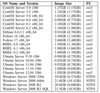
In this section, we present our findings on content similarity between VM disk images. We mainly studied VMware images, and some Amazon machine images (AMIs). We collected about 50 different VM images (Linux- and Unix-based OSs) from [15] and 10 images from [16]; some of them are listed in Table I.
We used the Bloom-filter-based fingerprints (described in Section 2) in all of our comparisons. We generated a finger-print for each VM disk image. To calculate content similarity between two images, we calculated the intersection of the corresponding fingerprints. In our experiments, content sim-ilarity estimates based on the fingerprints were within 1% of the actual content similarities. VM disk images often have duplicate blocks, but the fingerprints allow us to determine the total size of the VM disk image without the duplicate blocks. In Table I, in the second column, we first show the size of each stored VM disk image on the file system (size with duplicate blocks), and then, in parentheses, its size without duplicate blocks.
A. Comparison between Base Virtual Disk Images
In this section, we discuss the content similarity results between the base VM disk images. Results of our comparisons are shown in Table II. We found that VMs with different
OS Name and Version Image Size FS
CentOS Server 5.0 i386 1.27GB (1.13GB) ext3 CentOS Server 5.5 i386 1.32GB (1.17GB) ext3 CentOS Server 5.8 x86 64 1.62GB (1.40GB) ext3 CentOS Server 6.0 x86 64 0.98GB (0.77GB) ext3 CentOS Server 6.1 x86 64 2.16GB (1.94GB) ext3 CentOS Server 6.2 x86 64 2.18GB (1.96GB) ext3 Debian 6.0.2.1 x86 64 0.91GB (0.76GB) ext3 Fedora 16 x86 64 2.49GB (2.24GB) ext3 Fedora 17 x86 64 2.66GB (2.40GB) ext3 RHEL 6.0 x86 64 1.50GB (1.36GB) ext4 RHEL 6.1 x86 64 1.80GB (1.66GB) ext4 RHEL 6.2 x86 64 1.80GB (1.70GB) ext4 Ubuntu Server 9.10 i386 0.90GB (0.75GB) ext3 Ubuntu Server 10.04 i386 0.85GB (0.74GB) ext3 Ubuntu Server 11.04 i386 0.92GB (0.78GB) ext3 Ubuntu Server 11.10 i386 1.00GB (0.84GB) ext3 Ubuntu Server 12.04 i386 1.05GB (0.85GB) ext3 Windows Server 2008 32bit 19.0GB (6.57GB) NTFS Windows Server 2008 64bit 21.0GB (10.1GB) NTFS Windows Server 2008 R2 20.0GB (8.60GB) NTFS Windows Server 2008 R2 SQL 21.5GB (10.5GB) NTFS
TABLE I
VMDISK IMAGES FROM[15]AND[16].
VM 1 VM 2 Shared CentOS 5.0 33% CentOS 5.5 32% 376MB CentOS 5.0 28% CentOS 5.8 23% 376MB CentOS 5.0 0% CentOS 6.0 – 6.2 0% 0MB CentOS 5.5 38% CentOS 5.8 32% 444MB CentOS 5.5 0% CentOS 6.0 – 6.2 0% 0MB CentOS 5.8 0% CentOS 6.0 – 6.2 0% 0MB CentOS 6.0 36% CentOS 6.1 15% 280MB CentOS 6.0 28% CentOS 6.2 12% 220MB CentOS 6.1 60% CentOS 6.2 60% 1.15GB Fedora 16 33% Fedora 17 30% 720MB RHEL 6.0 56% RHEL 6.1 46% 730MB RHEL 6.0 50% RHEL 6.2 38% 650MB RHEL 6.1 56% RHEL 6.2 53% 890MB Ubuntu 9.10 0% Ubuntu 10.04 – 12.04 0% 0MB Ubuntu 10.04 18% Ubuntu 11.04 17% 132MB Ubuntu 10.04 14% Ubuntu 11.10 12% 100MB Ubuntu 10.04 7.6% Ubuntu 12.04 6.6% 56MB Ubuntu 11.04 26% Ubuntu 11.10 24% 204MB Ubuntu 11.04 13% Ubuntu 12.04 12% 100MB Ubuntu 11.10 16% Ubuntu 12.04 16% 136MB Win 2008 32b 67% Win 2008 64b 44% 4.4GB Win 2008 32b 23% Win 2008 R2 17% 1.5GB Win 2008 32b 23% Win 2008 R2 SQL 14% 1.5GB Win 2008 64b 31% Win 2008 R2 36% 3.1GB Win 2008 64b 31% Win 2008 R2 SQL 30% 3.1GB Win 2008 R2 96% Win 2008 R2 SQL 79% 8.3GB TABLE II
CONTENT SIMILARITY BETWEENVMS.
OSs have no content in common; therefore, such pairs are not displayed in the table. In Table II, we show the comparison between base VM disk images with the same OS but different version numbers. The sizes of the VM disk images are shown in Table I, and the last column of Table II shows the amount of data that is common to VM 1andVM 2. The percentages of content similarity (columns 2 and 4) between images are calculated by comparing the Shared column in Table II against the Image Size column in Table I. For example, consider the first row of Table II as an example. The size of the CentOS
VM Name Image Size Shared Size
CentOS Server 5.0 2.3GB (1.9GB) 1.0GB CentOS Server 5.5 2.4GB (1.8GB) CentOS Server 6.1 3.5GB (2.9GB) 2.2GB CentOS Server 6.2 3.7GB (2.9GB)
TABLE III
CONTENT SIMILARITY: CENTOSSERVERS WITH ALL UPDATES.
Server 5.0 is 1.27GB (1.13GB), where 1.13GB is the size of the image without the duplicate blocks. The shared size between CentOS Server 5.0 and CentOS Server 5.5 is 376MB, which does not include duplicate blocks either. Hence, to calculate what percent of CentOS Server 5.0’s content appears in CentOS Server 5.5, we take 1376.13M BGB = 0.33or 33%.
Content similarity for Red Hat Enterprise Linux VMs is between 38% and 56%; for Fedora VMs, content similarity is 30%. Content similarities are fairly high, considering that the VMs have different version numbers. Later, we will discuss how content similarity is higher for VMs that have the same OS and version numbers, but have different packages installed to perform different tasks. Content similarity among CentOS Servers 5.0 through 5.8 is also approximately 30%. Further, as shown in Table II, there is no content similarity between CentOS VMs with version numbers 5.8 and earlier, and those with version numbers 6.0 and later. There is much higher content similarity between CentOS Servers 6.1 and 6.2 (1.15GB or 60%). The content similarity is much higher between VMs with close version numbers. It is not shown in Table II, but the content similarity between CentOS Servers 5.5 and 5.7 is 550MB, while the content similarity between CentOS Servers 5.5 and 5.8 is 444MB. CentOS Server 6.0 is a minimal version of the server; hence, there is very low content similarity between it and the later versions of CentOS Server. For most OSs, we note that content similarity goes down drastically after each major release. That was also true for Ubuntu VMs where major releases of Ubuntu Server were 8.04 and 10.04. Ubuntu Server 8.04 and Ubuntu Server 10.04 are Long Term Support (LTS) releases of Ubuntu. As with CentOS Server VMs, there was no content similarity between VMs with version numbers prior to 10.04, and the ones with 10.04 and later. Indeed, compared to other OSs, content similarity between different versions of Ubuntu Server VMs is very low. For Windows servers, Windows Server 2008 R2 was re-leased after Windows Server 2008, and is a 64-bit-only OS. Hence, the content similarity between R2 and Windows Server 2008 64-bit is higher than the content similarity between R2 and Windows Server 2008 32-bit. The Windows Server 2008 R2 SQL VM has SQL Server Express 2008 & IIS installed. The content similarity between R2 and R2 SQL is very high, even after R2 SQL has been customized with new applications. So far in this paper, we have compared base VMs. For CentOS Servers, content similarity increased after the latest updates were applied. Table III shows comparisons after application of updates to CentOS Servers. Content similarity between CentOS Server 5.0 and CentOS Server 5.5 increased
Ubuntu packages
Web Servers Apache2 Web Server, Squid Proxy Server
Databases MySQL, PostgreSQL
Wiki Apps Moin Moin, MediaWiki
File Servers FTP Server, CUPS Print Server
Email Services Postfix, Exim4
Version Control System Subversion, CVS, Bazaar
TABLE IV
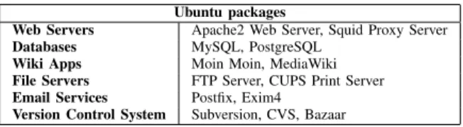
LIST OF PACKAGES USED TO CUSTOMIZEUBUNTU SERVERVMS.
Ubuntu Version Avg. Similarity Avg. Size
Ubuntu Server 10.04 680MB 920MB Ubuntu Server 11.10 925MB 1.15GB Ubuntu Server 12.04 870MB 1.09GB
TABLE V
AVERAGE CONTENT SIMILARITY BETWEEN CUSTOMIZEDUBUNTU SERVERVMS.
from about 33% to 53%. For CentOS Servers 6.1 and 6.2, it went up from 60% to 75%. This gain comes at a cost, because the overall sizes of the CentOS VMs increased by about a GB after the updates were applied. Similar behavior was not observed for other OSs.
B. Comparison between Customized VMs
In this section, we compare VMs that have the same OS and version numbers, but are customized with different packages. In the previous section, we saw that content similarity between VMs with the same OSs but different versions is not always very high. But in data centers, hundreds of thousands of VMs are deployed daily, and hence there will be opportunities to schedule VMs with both the same OSs and the same versions at the same hosts. Typically, certain versions of each OS will be more widely used than other versions, and users may have their own customized VMs of that version. To compare these types of VMs, we started with the same base image, installed different sets of packages on that image to create customized VMs, and measured the content similarity between them.
Table IV describes the set of packages we used to customize Ubuntu VMs. For each version of Ubuntu Server, we created three VMs from the same base image. Then, for each of the VMs, we installed different subsets of the packages shown in Table IV. We selected at least one package from each category in the table for each custom VM. The comparison results are shown in Table V. In the last column of that table, we display the average sizes of the three customized VMs after installation of the packages, without the duplicate blocks. In the second column, we averaged the content similarities in each pair of VMs. Even after we installed very different sets of packages, the content similarity between VMs with the same OS versions remained very high.
For Fedora VMs, we followed a similar technique to cus-tomize the VMs. The results, shown in Table VI, are very similar to the Ubuntu results.
V. EXPERIMENTS
To evaluate the effectiveness of the content-based schedul-ing algorithms in lowerschedul-ing network traffic in data centers, we
Fedora Version Avg. Similarity Avg. Size
Fedora 16 2.45GB 3.1GB
Fedora 17 2.3GB 3GB
TABLE VI
AVERAGE CONTENT SIMILARITY BETWEEN CUSTOMIZEDFEDORAVMS.
did a simulation of a deployment of VMs in a data center. In this section, we describe the simulator, simulation parameters, and the simulation results.
A. Simulation Setup
For our simulation, we generated a VM deployment trace. The trace consisted of all the VMs deployed during the simulation. Each VM deployment event in the trace contained the following information: start and termination time, OS name and version number, and instance type. We describe how we assigned each of these properties to the VMs next. Start and termination times are described in Section V-A1; OS name and version number assignments are covered in Section V-A2; and instance types are described in Section V-A3.
1) VM deployment rates: We wanted to use realistic esti-mates of how many VMs were getting deployed at any given time of day. We followed the technique described in [2] to estimate the VM deployment rates. According to [2], for AWS data centers, given two AMI IDs and their start times, it is possible to calculate the number of VMs that were deployed in the same AWS data center between the start times of the two VMs. Following that technique, we periodically deployed new VM in the AWS Virginia data center every five minutes for 24 hours. From the resulting data, we were able to gather the number of VMs deployed in each 5-minute period in one day. We used those data in generating start times and the number of VMs to deploy in our simulation.
Although we were able to estimate the start times of VMs, we could not perform any similar experiment to estimate the duration or termination times of the VMs in commer-cial clouds. Using all the information we had available, we estimated that a small portion of the VMs last only a few hours, and another small portion of the VMs stay in operation for weeks to months. Hence, in our simulation, we set the duration for 25% of the VMs to be between a few minutes to a couple of hours; specifically, we uniformly selected time lengths between 5 minutes and 2 hours for those VMs. We also set 15% of the VMs to have a duration between one day and a few weeks. Since we simulated one week of VM deployments in a data center, any durations longer than one week had the same effect. For the rest of the VMs, meaning the majority of the VMs, we uniformly selected running times between two hours and 15 hours.
2) OS distribution: Since many websites are hosted in cloud data centers, we used the distribution of Web server OSes listed in [17] to assign OSes to VMs in our simulation. However, [17] does not provide a breakdown of distributions by version numbers. Therefore, we assigned much higher probabilities to the latest versions of the OSes in our
sim-Sto rag e Rac k Sto rag e Rac k Switch Switch Storage Cluster Co m pu te Rac k Co m pu te Rac k Switch Switch Compute Cluster Co m pu te Rac k Co m pu te Rac k Switch Switch Compute Cluster
Switch Switch Switch Switch Switch Switch Switch Switch
Fig. 4. Data center architecture
Instance type Resource Usage
Small 1.70GB RAM, 1 Compute Unit Medium 3.75GB RAM, 2 Compute Units Large 7.50GB RAM, 4 Compute Units XLarge 15.0GB RAM, 8 Compute Units
TABLE VII
DESCRIPTION OFVMINSTANCE TYPES
ulation trace than to the older versions (e.g., 70% for CentOS 6.2, 75% for Fedora 17, and 50% for Ubuntu 12.04).
3) VM instance types: VM instance types specify the resource allocation for VMs when they are deployed. Table VII shows different instance types. Like the duration times of VMs, information about VM instance type distributions in data centers is not publicly available. Hence, we assigned instance types to VMs in our simulation based on the numbers that were provided in [18].
4) Data center: In our simulation, we simulated deploy-ment of VMs in a single data center. We impledeploy-mented a data center architecture that was inspired by a real cloud architecture deployed by a major U.S. ISP and is shown in Figure 4. Each node was represented by a blade server, and each rack contained several blade servers. In our deployment, the amount of RAM was the limiting resource of the blade servers; therefore, the RAM determined the number of VMs that could be hosted on a single blade server. The blade servers in our data center were equipped with 140GB of RAM. Table VII shows the resource requirements for each VM instance type. As shown in the table, we decided to use EC2 Compute Units as the measure of CPU requirements. Given the blade server specs and Table VII, we could deploy at most 9 XLarge VMs simultaneously on a single blade (compute node). Alternatively, we could have a combination of at most 2 XLarge, 6 Large, and 17 Medium VMs deployed at the same time (2·15 + 6·7.5 + 17·3.75 = 138.75≤140). During the simulation, at a VM’s termination time, we removed the VM from the node, and the resources occupied by the VM became available again.
5) Content similarity: During the simulation, the schedul-ing algorithm decisions were based on content similarity
0 50 100 150 200 250 300 350
Random Greedy Dedicated (1) Dedicated (5) Dedicated (10) Optimal
Transferred Data (TB)
64GB RAM Node 140GB RAM Node
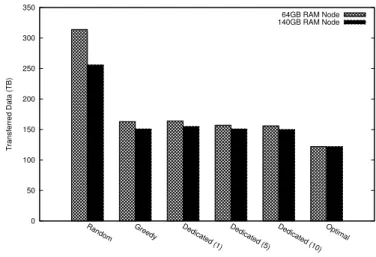
Fig. 5. Total amount of data transferred for different scheduling algorithms. The total size of all VMs deployed is 578TB, and the size of all VMs with duplicate disk blocks eliminated is 455TB. The confidence interval bound in either direction is less than 1TB for algorithms involving randomness (Dedicated, Random).
between the VM being scheduled and the rest of the VMs running on the compute nodes. We calculated the content similarity between VMs as follows. When there was a request from the scheduling algorithm to calculate content similarity between V M1 and V M2, we looked at two things. First, if
the two VMs had different OSs, we returned zero content similarity. If the two VMs had the same OS but different versions, we returned the size of the shared content noted in Table II. If the request was for two VMs with the same OS and the same version, then we treated the two VMs as customized VMs based on the same base image. In Section IV, we show content similarity only between customized VMs for Ubuntu and Fedora VMs, but we have collected similar results for the VMs with other OSs as well. For customized VMs of each OS and version number, we have four different content similarity values for each pair of comparisons. In response to a content similarity request for a pair of customized VMs, we returned a number uniformly chosen between the minimum and maximum of the four comparison values.
B. Simulation Results
We ran the simulation with different scheduling algorithms. The greedy and dedicated node algorithms are described in Section III. We tried the dedicated node algorithm with
n = 1,5, and 10, where n is the number of nodes we evaluated to find the greatest content similarity. We also used a random algorithm, which worked as follows. A random node in the data center was selected, and a local VM from that node that had the highest content similarity to the VM being scheduled was used to determine which other blocks needed to be transferred from the new VM to that selected node.
In the simulation, the amount of data transferred was calculated as follows. LetV Mnew be the VM disk image we
were transferring to a node. The VM on that node with the highest content similarity toV MnewisV Mlocal. Letsizeorig
be the size of the V Mnew on the file system; sizedist be
the size of the V Mnew without the duplicate blocks; and sizesharedbe the size of shared content betweenV Mnewand V Mlocal. To transferV Mnew, it is only necessary to transfer
missing blocks to the destination, and each unique disk block is transferred only once. Hence, the amount of data transferred to the destination is sizedist−sizeshared.
The simulation results are shown in Figure 5. The sim-ulations consisted of deploying VMs for a duration of one week. Initially, we started with a data center with no VMs running. We ran simulations with two data center setups, one with 140GB RAM nodes, and another with 64GB RAM nodes. We used the 64GB nodes to see how node RAM capacities affected the different algorithms. Each run of the simulation was performed on the same trace file that we generated.
The total size of all the deployed VMs was 578TB, and the size without the duplicate blocks was 455TB. Figure 5 shows the total amount of data transferred while the virtual disk images was being copied during the VM deployments. In the bars labeled Optimal, we show how much data would have to be transferred if, during the deployment of each VM, there existed another VM with the highest possible content similarity, and the new VM was scheduled on the same node as the other VM. Such a scenario cannot be guaranteed in a real scheduling algorithm execution, because there is no guarantee that there will be another VM with the highest content similarity running when each VM is deployed or that there is space on the compute node with this VM.
It can be seen in Figure 5 that the scheduling algorithms performed better when 140GB RAM nodes were used. The difference is the largest for the random algorithm. That was expected, because 140GB RAM nodes can host more than twice as many VMs as the 64GB RAM nodes can. In the random algorithm, VMs are scheduled to random nodes. Since a 140GB RAM node can host more VMs than a 64GB RAM node can, a randomly chosen node is more likely to have a VM with higher content similarity. Other algorithms are not affected as much, because the scheduler in the other algorithms evaluates multiple nodes to find the one with the highest content similarity.
From here on, we will refer to the results from the sim-ulation with the 140GB RAM nodes. The random algorithm transferred 256TB, where the total size of the VMs in the file system was 578TB. Even the random algorithm decreases the amount of transferred data by1−256T B
578T B = 56%. The dedicated
node algorithms with N= 1,5,and10decreased the amount of data transferred by 1− 155T B
578T B = 73.2%, 1−
151T B
578T B =
73.9%, and 1 − 150T B
578T B = 74%, respectively. The greedy
algorithm decreased the amount by 1−151T B
578T B = 73.9%.
The greedy algorithm performed only as well as the ded-icated nodes algorithm with N = 5. The greedy algorithm evaluates all the nodes in the data center, while the dedicated nodes algorithm only evaluates 5 nodes with the same OS as the VM being deployed. Hence, in terms of how long it takes the scheduling algorithm to find the destination node, the dedicated node algorithms have a big advantage over the
greedy algorithm. But, as we mentioned earlier, the greedy algorithm does not have the same restriction as the dedicated node algorithm, where each node can only run VMs with the same OS.
There was a small gain in going from N = 1 to N = 5
in the dedicated node algorithms, and an even smaller gain in going from N = 5 toN = 10. That tells us that we do not need to evaluate many dedicated nodes to find VMs with high content similarity.
The results are very promising. Transferring 73% less network data between racks inside a data center is a big improvement. The cost is that there is extra computation involved in transferring the VMs to the destination nodes. If the network bandwidth is the bottleneck inside a data center, then the benefits of the content-based scheduling algorithm are significant.
VI. LESSONSLEARNED
There are several important lessons to be learned from Section V. One of the biggest is that even without em-ploying computation-intensive scheduling algorithms, we can still achieve high network bandwidth savings using content-based scheduling of VMs in data centers. The dedicated node algorithm with N = 1 performed almost as well as the one withN = 5. That tells us that if we dedicate each compute node to host VMs with the same OS (but not necessarily the same OS release version), then a scheduling algorithm can perform very well by just randomly selecting a compute node whose OS matches the VMs being scheduled. In other words, the algorithm doesn’t have to examine more than one compute node to find high content similarity between VMs being scheduled and VMs already running on dedicated compute nodes.
The results from Sections IV and V also suggest that content similarity between VMs can sometimes be found through techniques even simpler than Bloom filters. For example, just matching OS name and release versions of VMs can sometimes lead to significant content similarity between the VMs. The reason, as we saw in Section IV, is that most content similarity seems to exist between custom VMs with the same origin OS and version.
The above discoveries make it easy to plug content-based scheduling into existing cloud data centers, and can lead to noticeable network bandwidth savings without involving too much extra computation cost.
VII. CONCLUSION
Cloud computing makes it easy to deploy and terminate vir-tual machines as desired, and the pay-for-what-you-use billing model encourages users to keep VMs running only when needed. As a result, hundreds of thousands of VMs may be deployed in a day in a large cloud data center. To deploy a VM, it is necessary to transfer the VM disk image from a storage rack to be executed on a compute node on a compute rack. As VM images can be tens of GB in size, intra-data-center traffic due to VM deployments can put a significant strain on the
data center network infrastructure. In this paper, we presented a novel scheduling algorithm that utilizes similarity between VM disk images, a similarity that is maintained for VMs with the same OS version even if the OS is customized and is in use. We quantified the similarities between VM images and showed that the similarity can be as high as 60–70%, or even over 90% in some cases. We demonstrated using a simulation that our scheduling algorithm can reduce the network utilized for a VM image transfer by over 70%. Such savings are significant enough to affect the networking design for cloud data centers, and definitely reduce network congestion and increase the available bandwidth for the VMs running in the cloud data center. Since the optimization results in colocation of VMs with shared pages on the same compute node, it also increases the benefits of using memory page sharing on the node resulting in better utilization of the often-bottlenecked memory resources.
REFERENCES
[1] H. Liu. Amazon data center size. Visited on November 9, 2012. [Online]. Available: http://huanliu.wordpress.com/2012/03/13/amazon-data-center-size/
[2] T. von Eicken. Amazon usage estimates. Visited on November 9, 2012. [Online]. Available: http://blog.rightscale.com/2009/10/05/amazon-usage-estimates/
[3] S. K. Bose, S. Brock, R. Skeoch, and S. Rao, “CloudSpider: Combining replication with scheduling for optimizing live migration of virtual machines across wide area networks,” in Proceedings of the 2011 11th IEEE/ACM International Symposium on Cluster, Cloud and Grid Computing (CCGrid). IEEE, 2011, pp. 13–22.
[4] S. Al-Kiswany, D. Subhraveti, P. Sarkar, and M. Ripeanu, “VMFlock: Virtual machine co-migration for the cloud,” inProceedings of the 20th International Symposium on High Performance Distributed Computing. New York, NY, USA: ACM, 2011, pp. 159–170. [Online]. Available: http://doi.acm.org/10.1145/1996130.1996153
[5] U. Deshpande, X. Wang, and K. Gopalan, “Live gang migration of virtual machines,” in Proceedings of the 20th International Symposium on High Performance Distributed Computing. New
York, NY, USA: ACM, 2011, pp. 135–146. [Online]. Available: http://doi.acm.org/10.1145/1996130.1996151
[6] K. Takahashi, K. Sasada, and T. Hirofuchi, “A fast virtual machine storage migration technique using data deduplication,” inProceedings of CLOUD COMPUTING 2012: The 3rd Int. Conf. on Cloud Computing, GRIDs, and Virtualization, 2012, pp. 57–64.
[7] K. Jin and E. L. Miller, “The effectiveness of deduplication on virtual machine disk images,” in Proceedings of SYSTOR 2009: The Israeli Experimental Systems Conference. New York, NY, USA: ACM, 2009, pp. 7:1–7:12. [Online]. Available: http://doi.acm.org/10.1145/1534530.1534540
[8] C. Peng, M. Kim, Z. Zhang, and H. Lei, “VDN: Virtual machine image distribution network for cloud data centers,” in Proceedings of IEEE INFOCOM, 2012, 2012, pp. 181–189.
[9] T. Wood, G. Tarasuk-Levin, P. Shenoy, P. Desnoyers, E. Cecchet, and M. D. Corner, “Memory buddies: Exploiting page sharing for smart colocation in virtualized data centers,” in Proceedings of the 2009 ACM SIGPLAN/SIGOPS International Conference on Virtual Execution Environments. New York, NY, USA: ACM, 2009, pp. 31–40. [Online]. Available: http://doi.acm.org/10.1145/1508293.1508299
[10] A. Arcangeli, I. Eidus, and C. Wright, “Increasing memory density by using KSM,” inProceedings of the Linux Symposium, 2009, pp. 19–28. [11] D. Gupta, S. Lee, M. Vrable, S. Savage, A. C. Snoeren, G. Varghese, G. M. Voelker, and A. Vahdat, “Difference engine: Harnessing memory redundancy in virtual machines,” Commun. ACM, vol. 53, no. 10, pp. 85–93, Oct. 2010. [Online]. Available: http://doi.acm.org/10.1145/1831407.1831429
[12] G. Mił´os, D. G. Murray, S. Hand, and M. A. Fetterman, “Satori: Enlightened page sharing,” inProceedings of the 2009 Conference on USENIX Annual Technical Conference. USENIX Association, 2009. [13] Openstack. Visited on November 10, 2012. [Online]. Available:
http://www.openstack.org/
[14] A. Broder and M. Mitzenmacher, “Network applications of Bloom filters: A survey,” inInternet Mathematics, vol. 1, no. 4. Taylor & Francis, 2004, pp. 485–509.
[15] VMware images. Visited on November 12, 2012. [Online]. Available: http://www.thoughtpolice.co.uk/vmware/
[16] Amazon Web Services. [Online]. Available: https://aws.amazon.com/ [17] Usage of operating systems for websites. Visited on November 13,
2012. [Online]. Available: http://w3techs.com/technologies/overview/-operating system/all
[18] T. von Eicken. More servers, bigger servers, longer servers, and 10x of that. Visited on November 9, 2012. [Online]. Available: http://blog.rightscale.com/2010/08/04/more-bigger-longer-servers-10x/