Artificial Neural Network Parameter Tuning
Framework For Heart Disease Classification
M. Haider Abu Yazid Faculty of Computing Universiti Teknologi Malaysia
(UTM) Johor Bahru, Malaysia [email protected]
Muhammad Haikal Satria Faculty of Bioscience and
Medical Engineering Universiti Teknologi Malaysia
(UTM) Johor Bahru, Malaysia
Shukor Talib Faculty of Computing Universiti Teknologi Malaysia
(UTM) Johor Bahru, Malaysia
Novi Azman Faculty of Engineering and
Science Universitas Nasional
Jakarta, Indonesia [email protected]
Abstract— Heart Disease are among the leading cause of death worldwide. The application of artificial neural network as decision support tool for heart disease detection. However, artificial neural network required multitude of parameter setting in order to find the optimum parameter setting that produce the best performance. This paper proposed the parameter tuning framework for artificial neural network. Statlog heart disease dataset and Cleveland heart disease dataset is used to evaluate the performance of the proposed framework. The results show that the proposed framework able to produce high classification accuracy where the overall classification accuracy for Cleveland dataset is 90.9% and 90% for Statlog dataset.
Keywords—artificial neural network, heart disease classification, artificial neural network parameter tuning, statlog heart dataset, cleveland heart dataset.
I. INTRODUCTION
Heart disease describes a range of conditions that affect your heart. Heart disease is under umbrella of cardiovascular disease in which are the leading cause of death worldwide where more people die from cardiovascular diseases compared to any other causes annually. Mortality for heart disease is projected to be increase to reach 23.3 million by the year of 2030 where heart disease will remain to be the leading cause of death for human. It became imperative to diagnose the presence of heart disease in the early stages in order to contain the disease from worsening. The early detection of heart disease can help the patient to adjust lifestyle and also help the medical professionals to prescribe appropriate medicine. However, the diagnosing patient with the presence of heart disease can be challenging where it depends on medical professional’s experience and intuition [12,13]. It is imperative for medical professionals to have a system that can help them predict and classify the patient who have high risk of getting heart disease.
The implementation of machine learning algorithm can help medical professionals in diagnosing the presence of heart
disease in the patient. Machine learning algorithm have become very popular for solving classification problems where it is capable of mapping the relationship between variables or attributes with minimal human effort
Artificial Neural Network (ANN) are among the most popular machine learning algorithm where it proves to be powerful tools for mapping nonlinear data and are known to be useful in solving nonlinear problems where the rules to solve the problem is difficult to obtain or unknown. However, Artificial Neural Network required a lot of parameter setting where parameter tuning often been done by trial and error. Feed forward back propagation neural network are the most commonly used type of artificial neural network and it requires the users to specify several parameters including the numbers of hidden layer, the numbers of hidden nodes, training algorithm and type of transfer function.
Presently, there are 13 types of training algorithm and 10 types of transfer function. The numbers of possible combination parameters that can be used can range from 1300 up until 130000 depending on the numbers of hidden layers specified by the users. The trial and error approach consuming enormous amount of time and does not guarantee the model to obtain the best possible classification accuracy.
This paper presents the parameter tuning framework for artificial neural network in order to find the optimal artificial neural network parameters for heart disease classification. Statlog heart disease dataset and Cleveland heart disease dataset obtain from UCI machine learning data repository are used to measure the performance of proposed parameter tuning framework.
II. ARTIFICIAL NEURAL NETWORK MODEL
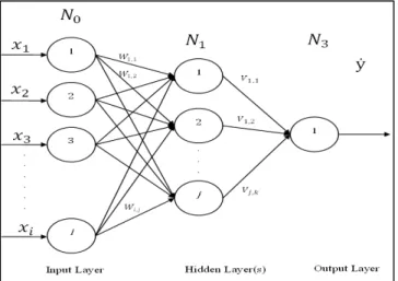
A neural network consists of an interconnected group of artificial neurons, and it processes information using a connectionist approach to computation. ANN has been implemented in various fields. In healthcare, ANN is implemented for clinical diagnosis, drug development, image analysis and signal analysis [1]. ANN had proven to be useful for modeling complex relationships between inputs and outputs or to find patterns in data. Basically, feed forward
neural network consists three main layers which are input layer, hidden layer and output layer. Input and output are usually consisting 1 layer and hidden layer could consist minimum 1 layer. Figure 1 shows the examples of feed forward neural network architecture. The numbers of input nodes and output nodes depends on the collected data while the numbers of hidden nodes for ANN are based on trial and error.
Figure 1 Basic Neural Network Architecture III. PARAMETER TUNING FRAMEWORK
Main parameters setting for Feed Forward Backpropagation consist of network structures (number of hidden layer and hidden nodes), training algorithm and types of transfer function. Additional parameter setting will be required depending on types of training algorithm used. Table 1 show the list of main parameters setting for Feed Forward Backpropagation Neural Network.
The numbers of hidden layer usually depending on the user definition. However, most of the previous research only use 1 or 2 hidden layers which enough to obtain the optimum performance. The increase number of hidden layers will increase the run time taken for neural network classification. Low numbers of hidden nodes may result in decreases of neural network classification accuracy. However, the high numbers of hidden nodes may increase neural network accuracy but will increase neural network run time. Previous research has proposed the number of hidden nodes to be at certain numbers depending on the number of input nodes. The number of hidden nodes recommended by previous research is according to “n/2”,”1n”,”2n” and “2n+1” where n is the number of input nodes [33]. However, this guideline does not guarantee the optimum number of hidden nodes required by the neural network to achieve optimum classification accuracy.
The proposed parameter tuning framework consist of several phase. The first phase selects the training algorithm while the second phase select transfer function. The third phase will select the hidden nodes number and the last phase will simulate the neural network using the parameters obtain in phase 1,2 and 3. In the last phase, the neural network will be simulated numerous time in order to find the best weight and bias that produce the highest classification accuracy.
Figure 2 shows the proposed artificial neural network parameter tuning framework.
Table 1: Feed Forward Backpropagation Parameter Setting
Hidden Layer
Hidden Nodes
Training Algorithm and Additional Parameters
Transfer Function
1-3 10-∞ a. BFGS quasi-Newton
backpropagation
b. Bayesian Regulation back
propagation
c. Conjugate gradient
backpropagation with Powell-Beale restarts
d. Fletcher-Reeves Conjugate
Gradient
e. Polak-Ribiére Conjugate Gradient
f. Gradient descent back propagation
•Learning Rate Parameter
g. Gradient descent with adaptive
learning rate back propagation
h. Gradient descent with momentum
•Learning Rate Parameter
•Momentum Parameter
i. Gradient descent with momentum
and adaptive learning rate back propagation
•Momentum Parameter
j. Lavenberg - Marquadt
k. One Step Secant
l. Resilient Back propagation
m. Resilient Back propagation
a. Hard Limit b. Symmetrical Hard Limit c. Linear d. Saturating Linear e. Symmetric Saturating Linear f. Log-Sigmoid g. Hyperbolic Tangent Sigmoid h. Positive Linear i. Softmax j. Competitive
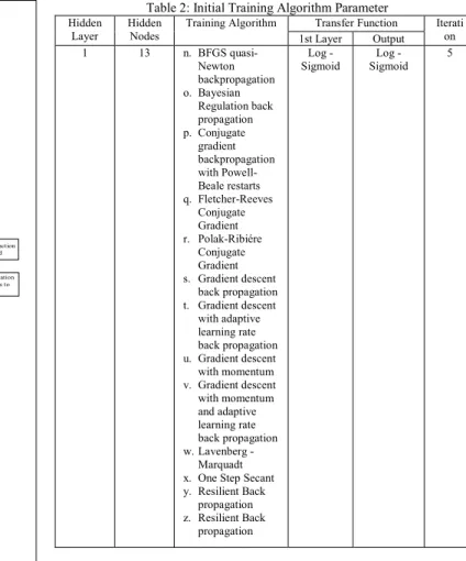
The first phase of the framework selects the suitable training algorithm for the each of the dataset. The most commonly used transfer function is used in the first phase. Table 2 shows the setup for first phase of proposed parameter tuning algorithm. In the first phase, all the training algorithm are simulated for five times of iteration to find the best performance from the different training algorithm. Each of the training algorithm will produce five different result for every iteration and the algorithm with the highest average overall accuracy will be chosen as a training algorithm. After the training algorithm is selected, phase 2 simulation is conducted.
For the phase 2, the transfer function combination has to be generated first. The transfer function combination is the possible combination of transfer function that can be use in hidden layer and output layer. This combination depending on the number of hidden layer and the number of transfer function that the users planned to use. This research uses 1 hidden layer with 10 types of transfer function. Table 3 shows the examples of transfer function combination. The initial neural network parameter and simulation parameter is defined after the transfer function combination is generated. Table 4 shows the neural network initial parameters and table 5 shows the simulation parameter. Neural network initial parameters specify the number of initial hidden nodes, training algorithm (selected from phase 1 of the framework), performance function and data partition setup. There 3 types of data used for simulation. Training dataset is used to train the network where the weight and bias is adjusted during training process. The validation dataset is used to validate the performance of the neural network. If the accuracy of validation dataset does not achieve the minimum accuracy desired by the user, the training process will be done again. The test dataset then will be used to evaluate the neural network model
Set Initial Training Algorithm Parameter Initialize Transfer Function Simulation Optimum Accuracy Achieved? Transfer Function Selected Reset Simulation Parameters to default Yes
Initialize Hidden Nodes Simulation Optimum Accuracy Achieved? Max Hidden Nodes Achieved? Increase “Hidden Nodes” based on “Hidden Nodes Increment” Decrease “Optimum Accuracy“ using “Accuracy Decrement” Reset Hidden Nodes to “Initial Hidden Nodes” No Yes Performance Analysis Training Algorithm Selected Decrease “Optimum Accuracy“ using “Optimum
Accuracy Decrement” No
Hidden Nodes Selected
Reset Test Parameters to default
Initialize All Selected Neural Networks
Parameters
Initialize Multi Training Neural Networks
Neural Network weight and bias selected
END START No Yes Initialize Training Algorithm Simulation Generate Transfer Function Candidates Set Neural Networks Initial Parameter Set Simulation Parameters Performance Analysis
Figure 2. Artificial Neural Network Parameter Tuning Framework The simulation parameter will be set once the neural network parameter is defined. The simulation parameter includes initial optimum accuracy, accuracy decrement, hidden nodes increment, and iteration for phase 2,3 and 4. Initial optimum accuracy is the user’s desired validation dataset accuracy. Accuracy decrement is the decrement of optimum accuracy and iteration is the number of iterations per phase. Hidden nodes increment is the parameter used to increase the hidden nodes value and the maximum hidden nodes is the maximum value of increased hidden nodes.
In phase 2, every combination of transfer function is simulated based on the number of iterations specifies by the users. Any combination of transfer function that achieved the “optimum accuracy” will be stored in the array. Optimum accuracy however will be changed according to “accuracy decrement” if there are no combination of transfer function achieved optimum accuracy during the specified iteration. The new “optimum accuracy” is calculated using equation (1).
= −
(1)
Table 2: Initial Training Algorithm Parameter
Hidden
Layer Hidden Nodes Training Algorithm 1st Layer Transfer Function Output Iteration
1 13 n. BFGS quasi-Newton backpropagation o. Bayesian Regulation back propagation p. Conjugate gradient backpropagation with Powell-Beale restarts q. Fletcher-Reeves Conjugate Gradient r. Polak-Ribiére Conjugate Gradient s. Gradient descent back propagation t. Gradient descent with adaptive learning rate back propagation u. Gradient descent with momentum v. Gradient descent with momentum and adaptive learning rate back propagation w. Lavenberg - Marquadt
x. One Step Secant
y. Resilient Back
propagation
z. Resilient Back
propagation
Log -
Sigmoid Sigmoid Log - 5
Where i is the current cycle of phase 2. The cycle will be repeated until the combination of transfer function that achieved “optimum accuracy” is found. After the phase 2 completed, the simulation parameter will be reset to the initial value specify by the users. The phase 3 will be execute after the simulation parameter is reset and neural network parameter is updated. The updated neural network parameter consists of the combination of transfer function that achieved the optimum accuracy in phase 2 and the training algorithm obtained from phase 1. For the phase 3, the initial hidden nodes values are set according to the number of dataset input. If the optimum accuracy is not achieved during the specifies iteration, the number of hidden nodes will be updated using equation (2).
ℎ = ℎ
+ ℎ
(2) Table 3: Examples of transfer function combination
1st Hidden Layer Transfer Function Output Layer Transfer Function
Hard Limit Hard Limit
Symmetrical Hard Limit Hard Limit
Linear Hard Limit
Saturating Linear Hard Limit
Symmetric Saturating Linear Hard Limit
Log-Sigmoid Hard Limit
Hyperbolic Tangent Sigmoid Hard Limit
Positive Linear Hard Limit
Softmax Hard Limit
Competitive Hard Limit
Hard Limit Symmetrical Hard Limit
Symmetrical Hard Limit Symmetrical Hard Limit
. . . . . .
. . . . . .
Hard Limit Competitive
. . . . . . Softmax Competitive Competitive Competitive
Table 4: Neural Network Initial Parameter
Initial Hidden Layer Initial Hidden Nodes Training Algorithm Performance Function Data Setup 1 13 Selected After Phase 1 Mean Squared
Error 1. Training Dataset 2. Validation Dataset 3. Test Dataset
Table 5: Simulation Parameter
Initial Optimum Accuracy
Accuracy
Decrement Hidden Nodes
Incremen t Maximum Hidden Nodes Iteration Phase 2&3 Iteration Phase 4 90 5 10 100 50 1000
Where j is the current cycle of phase 3. However, the optimum accuracy is not achieved even though the number of hidden nodes has increased equal to the number of “maximum hidden nodes”, the optimum accuracy will be updated using equation (1) and the new cycle of phase 3 will be restarted until the optimum accuracy is achieved. Phase 4 will be initiated once the optimum accuracy is achieved and the neural network parameters is updated with the optimum value of hidden nodes.
In phase 4, the neural network model using the parameters obtain in phase 1,2 and 3 will be simulated numerous times. Every iteration will be flagged with an “iteration identification” in order to find which iteration produce the best accuracy. Weight and bias for every iteration also is stored and flagged with “iteration identification”. After all iteration in phase 4 is completed, the algorithm will sort the results according to the validation dataset classification accuracy. The iteration identification will determine which iteration produce the highest accuracy of classification. The weight and bias of iteration with the highest classification will be extracted from the array. The neural network model with optimize parameters and the best weight and bias is simulated using test dataset for evaluation. The proposed framework uses two sets of heart disease data taken from UCI machine learning data repository. The Statlog dataset and Cleveland Heart dataset is used to evaluate the performance of proposed framework. The result of simulation then compared to the reported results published by the previous research. Dataset is partition into ratio of 80% for training, 10% for validation and 10% for testing.
IV. RESULTS
A. Parameter Tuning Result
Table 6 shows the parameter obtain from the proposed framework while table 7 shows classification result of heart disease dataset.
Table 6: Neural network parameter obtain by the proposed framework
Dataset Algorithm Training Hidden Layer Hidden Nodes 1st Hidden Transfer Function
Layer Output Layer
Cleveland Dataset Lavenberg - Marquadt 1 33 Saturating Linear Linear Statlog Dataset Fletcher-Reeves Conjugate Gradient
1 23 Symmetrical Hard Limit
Hyperbolic Tangent Sigmoid
Table 7: Heart disease classification accuracy
Dataset Training
Dataset Validation Dataset Test Dataset Accuracy Overall
Cleveland Dataset 91.1 80 100 90.9
Statlog Dataset 90.7 81.5 92.6 90.0
B. Comparison with Previous Research
Table 8 and 9 shows the comparison of classification accuracy for Cleveland and Statlog dataset between previously proposed algorithm and the proposed framework.
Table 8: Cleveland Dataset
Algorithm Accuracy (%)
Weighted Fuzzy [12] 57.85
Attribute weighted artificial immune system [19] 82.59
Artificial Immune System [19] 84.5
Modified Artificial Immune System [20] 87.43
IB1-4 [22] 50 C5.0 Tree [21] 53.1 J48 [21] 54.4 DKP C [21] 57.6 Random Forest [21] 58 InductH [23] 58.5 SVM C [21] 58.6 RBF [22] 60 FOIL [23] 64 MLP [22] 65.6 T2 [23] 68.1 1R [23] 71.4 IB1c [23] 74 K* [23] 76.7 Logistic regression [24] 77 C4.5 [25] 81.11 Naïve Bayes [25] 81.48 BNND [25] 81.11 BNNF [25] 80.96 AIRS [23] 84.5 AIRS [27] 84.5
Fuzzy-AIRS-Knn based system [26] 87
Artificial neural network (ANN) + Fuzzy neural network
(FNN) [29] 86.8
Combining of linear kernel F-score feature selection and
ANN [28] 80.74
Combining of RBF kernel F-score feature selection and
LS-SVM classifier [28] 83.7
SAS base-Neural networks ensemble [30] 89.01
FDT [31] 77.55
Structural least square twin support vector machine
(S-LSTSVM) [32] 87.82
Parameter Tuned ANN 90.9
Table 9: Statlog Dataset
Algorithm Accuracy (%) MARS-LR [14] 83.93 Weighted Fuzzy [12] 62 Fuzzy neurogenetic [15] 80 ANN-FNN [16] 87 CHAID [17] 76.6 CRT [17] 76.6 MLP [17] 83.3 RBFN [17] 84.6 ANFIS_LSLM [18] 76.7 ANFIS_LSGD [18] 75.6 IR [18] 71.4 T2 [18] 68.1 FOIL [18] 64 RBF [18] 60 InductH [18] 58.5
V. DISCUSSION
This paper proposed the artificial neural network parameter tuning for heart disease classification. The result shows that the proposed framework able to achieve high classification accuracy with the overall accuracy of 90.9% for Cleveland dataset and 90% of classification accuracy for Statlog dataset. The proposed framework also outperforms previous proposed algorithm. The parameter obtain by the proposed framework is differ from each dataset. It shows that different dataset may have different set of optimal parameters.
ACKNOWLEDGMENT
This research funded by University Technology of Malaysia (UTM) via Research University Grant (RUG) Tier 1 with vote no (PY/2017/00781).
REFERENCES
[1] Remzi M, Anagnostou T, Ravery V, Zlotta A, Stephan C, Marberger M, Djavan B. “An artificial neural network to predict the outcome of repeat prostate biopsies.” Urology. 2003 Sep;62(3):456-60
[2] Tu JV: “Advantages and disadvantages of using artificial neural networks versus logistic regression for predicting medical outcomes.”Journal of Clinical Epidemiol. 1996, 49: 1225-31. 10.1016/S0895-4356(96)00002-9.
[3] Demuth, Howard, and Mark Beale. "Neural Network Toolbox." For Use with MATLAB. The MathWorks Inc 2000 (1992).
[4] Lagu, Tara, Penelope S. Pekow, Meng-Shiou Shieh, Mihaela Stefan, Quinn R. Pack, Mohammad Amin Kashef, Auras R. Atreya, Gregory Valania, Mara T. Slawsky, and Peter K. Lindenauer. "Validation and Comparison of Seven Mortality Prediction Models for Hospitalized Patients With Acute Decompensated Heart FailureCLINICAL PERSPECTIVE." Circulation: Heart Failure 9, no. 8 (2016): e002912.
[5] Zhang, Guoqiang, B. Eddy Patuwo, and Michael Y. Hu. "Forecasting with artificial neural networks:: The state of the art." International journal of forecasting 14, no. 1 (1998): 35-62.
[6] Givertz, Michael M., John R. Teerlink, Nancy M. Albert, Cheryl A. Westlake Canary, Sean P. Collins, Monica Colvin-Adams, Justin A. Ezekowitz et al. "Acute decompensated heart failure: update on new and emerging evidence and directions for future research." Journal of cardiac failure 19, no. 6 (2013): 371-389. [7] Lee, Douglas S., Peter C. Austin, Jean L. Rouleau, Peter
P. Liu, David Naimark, and Jack V. Tu. "Predicting mortality among patients hospitalized for heart failure: derivation and validation of a clinical model." Jama 290, no. 19 (2003): 2581-2587.
[8] Amato, Filippo, Alberto López, Eladia María Peña-Méndez, Petr Vaňhara, Aleš Hampl, and Josef Havel. "Artificial neural networks in medical diagnosis." Journal of applied biomedicine 11, no. 2 (2013): 47-58. [9] Martin T. Hagan , Howard B. Demuth , Mark Beale,
“Neural network design.” PWS Publishing Co., Boston, MA, 1997
[10] Demuth, Howard, and Mark Beale. "Neural Network Toolbox." For Use with MATLAB. The MathWorks Inc 2000 (1992).
[11] Farmakis, Dimitrios, et al. "Acute heart failure: epidemiology, risk factors, and prevention." Revista Española de Cardiología (English Edition) 68.3 (2015): 245-248.
[12] Anooj, P. K. "Clinical decision support system: Risk level prediction of heart disease using weighted fuzzy rules." Journal of King Saud University-Computer and Information Sciences 24, no. 1 (2012): 27-40.
[13] Hedeshi, N. Ghadiri, and M. Saniee Abadeh. "Coronary artery disease detection using a fuzzy-boosting PSO approach." Computational intelligence and neuroscience 2014 (2014): 6.
[14] Y. E. Shao, C.-D. Hou, and C.-C. Chiu, “Hybrid intelligent modeling schemes for heart disease classification,” Applied Soft Computing Journal, vol. 14, pp. 47–52, 2014.
[15] K.Vijaya,H. K.Nehemiah,A.Kannan,
andN.G.Bhuvaneswari, “Fuzzy neuro genetic approach for predicting the risk of cardiovascular diseases,” International Journal of Data Mining, Modelling and Management, vol. 2, no. 4, pp. 388–402, 2010.
[16] H. Kahramanli and N. Allahverdi, “Design of a hybrid system for the diabetes and heart diseases,” Expert Systems with Applications, vol. 35, no. 1-2, pp. 82–89, 2008.
[17] Nahato, Kindie Biredagn, Khanna Nehemiah Harichandran, and Kannan Arputharaj. "Knowledge mining from clinical datasets using rough sets and backpropagation neural network." Computational and mathematical methods in medicine 2015 (2015).
[18] Sagir, Abdu Masanawa, and Saratha Sathasivam. "A Novel Adaptive Neuro Fuzzy Inference System Based Classification Model for Heart Disease Prediction." Pertanika Journal of Science & Technology 25, no. 1 (2017).
[19] Polat, K. , Sahan, S. , Kodaz, H. , & Günes, S. (2005). A new classification method to diagnosis heart disease: Supervised artificial immune system (AIRS). In Pro- ceedings of the Turkish symposium on artificial intelligence and neural networks (TAINN).
[20] Ozsen, S. , & Gunes, S. (2009). Attribute weighting via genetic algorithms for at- tribute weighted artificial immune system (AWAIS) and its application to heart disease and liver disorders problems. Expert Systems with Applications, Elsevier, 36 (1), 386–392
[21] Fern´andez-Delgado M, Cernadas E, Barro S, Amorim D (2014) Do we need hundreds of classifiers to solve real world classification problems? J Mach Learn Res 15:3133–3181
[22] Polat K, G¨unes S, Tosun S (2006) Diagnosis of heart disease using artificial immune recognition system and fuzzy weighted pre-processing. Pattern Recogn 39(11):2186–2193.
[23] Das R, Turkoglu I, Sengur A (2009) Effective diagnosis of heart disease through neural networks ensembles. Expert Syst Appl 36(4):7675–7680.
[24] Detrano R, Janosi A, Steinbrunn W, Pfisterer M, Schmid JJ, Sandhu S, Guppy KH, Lee S, Froelicher V (1989) International application of a new probability algorithm for the diagnosis of coronary artery disease. Am J Cardio 64(5):304–310.
[25] Cheung N (2001) Machine learning techniques for medical analysis. School of Information Technology and Electrical Engineering, BSc Thesis, University of Queenland.
[26] Polat K, Sahan S, G¨unes S (2007) Automatic detection of heart disease using an artificial immune recognition system (AIRS) with fuzzy resource allocation mechanism and k-nn (nearest neighbour) based weighting preprocessing. Expert Syst Appl 32(2):625– 631.
[27] Polat K, G¨unes S, Tosun S (2006) Diagnosis of heart disease using artificial immune recognition system and fuzzy weighted pre-processing. Pattern Recogn 39(11):2186–2193.
[28] Polat K, G¨unes S (2009) A new feature selection method on classification of medical datasets: Kernel f-score feature selection. Expert Syst Appl 36(7):10,367– 10,373.
[29] Kahramanli H, Allahverdi N (2008) Design of a hybrid system for the diabetes and heart diseases. Expert Syst Appl 35(1-2):82–89.
[30] Das R, Turkoglu I, Sengur A (2009) Effective diagnosis of heart disease through neural networks ensembles. Expert Syst Appl 36(4):7675–7680
[31] El-Bialy R, Salamay MA, Karam OH, Khalifa ME (2015) Feature analysis of coronary artery heart disease data sets. Procedia Comput Sci 65:459–468.
[32] Xu Y, Pan X, Zhou Z, Yang Z, Zhang Y (2015) Structural least square twin support vector machine for classification. Appl Intell 42(3):527–536.
[33] Zhang, Guoqiang, B. Eddy Patuwo, and Michael Y. Hu. "Forecasting with artificial neural networks:: The state of the art." International journal of forecasting 14, no. 1 (1998): 35-62