Hierarchical Multiclass Topic Modelling
with Prior Knowledge
Master’s Thesis submitted to
First Supervisor: Prof. Dr. Wolfgang K. Härdle
Second Supervisor: Prof. Dr. Cathy Yi-Hsuan Chen
Ladislaus von Bortkiewicz Chair of Statistics C.A.S.E. – Center for Applied Statistics
and Economics
Humboldt–Universität zu Berlin
by
Ken Schröder
(568399)
in partial fulfillment of the requirements for the degree of
Master of Science (Statistics)
Abstract
A new multi-label document classification technique called CascadeLDA is introduced in this thesis. Rather than focusing on discriminative modelling techniques, CascadeLDA extends a baseline generative model by incorporating two types of prior information. Firstly, knowledge from a labeled training dataset is used to direct the generative model. Secondly, the implicit tree structure of the labels is exploited to emphasise discriminative features between closely related labels. By segregating the classification problem in an ensemble of smaller problems, out-of-sample results are achieved at about 25 times the speed of the baseline model. In this thesis, CascadeLDA is performed on datasets with academic abstracts and full academic papers. The model is employed to assist authors in tagging their newly published articles.
Keywords: Bayesian, Gibbs sampling, Latent Dirichlet Allocation, machine learning,
CONTENTS
Contents
1 Introduction 1
2 Latent Dirichlet Allocation 2
2.1 Conjugate Priors . . . 5
2.2 Collapsed Gibbs Sampling . . . 7
2.3 Variational Inference: Background . . . 10
2.4 Variational Inference in Latent Dirichlet Allocation . . . 13
2.4.1 Full Conditionals in LDA . . . 14
2.4.2 Variational Factors in LDA . . . 15
3 Incorporating Available Information 17 3.1 Extension 1: Labeled LDA . . . 17
3.2 Extension 2: Hierarchically Supervised LDA . . . 20
3.2.1 Generative Model . . . 21
3.2.2 Gibbs Sampling . . . 23
3.3 Extension 3: CascadeLDA . . . 25
4 Data and Preprocessing 27 5 Evaluation Methods and Experiment Setup 29 5.1 Challenges in Classification . . . 29
5.2 Metrics for Classification Quality . . . 31
5.3 Experiment Setup . . . 33
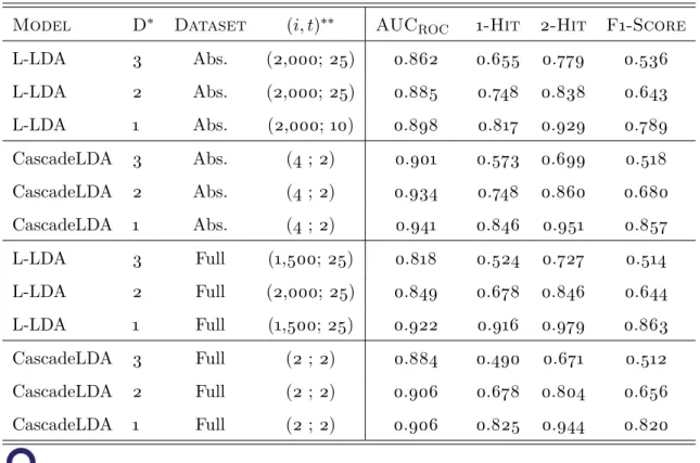
6 Results 35 6.1 L-LDA and CascadeLDA . . . 35
6.1.1 Number of Iterations . . . 37 6.1.2 Speed Assessment . . . 38 6.2 HSLDA . . . 39 7 Conclusion 40 7.1 Applications . . . 40 7.2 Future Research . . . 41
LIST OF FIGURES
List of Figures
1 Graphical model: LDA . . . 4
2 Graphical model: Labeled LDA . . . 18
3 Label structure: JEL code tree . . . 21
4 Graphical model: Hierarchically Supervised LDA . . . 22
5 Graphical model: CascadeLDA . . . 25
List of Tables
1 Definition of variables . . . 32 The ten most likely words for five JEL codes . . . 19
3 Summary statistics of the corpora . . . 28
1 Introduction
Automated text classification has been an active field of research for decades and is used in numerous applications. Despite its age, the field has gained prominence over the past decade. This is due to the increasing need to organise vast amounts of digital textual information and developments in machine learning techniques and computational power.
A number of equally valid interpretations of "automated text classification" prevail (Se-bastiani, 2002). The interpretations range from solely identifying categories in a body of documents to tagging documents according to pre-specified categories. In this thesis, we will focus on the latter interpretation. An extensive variety of methods exist to tag documents. Most of them use a dataset of labeled texts with which a model is trained to predict the category (categories) to which the text belongs. This training may involve neural networks (Nam et al., 2014), support vector machines (Joachims, 2002) or simpler methods like naive Bayes (McCallum and Nigam, 1998) to name a few.
In this research, Latent Dirichlet Allocation (LDA) (Blei et al., 2003) will be used as a baseline method. LDA is a "generative probabilistic model for collections of discrete data such as text corpora" (Blei et al., 2003, p. 993) and is an unsupervised machine learning algorithm. A common application of LDA is to identify latent semantic topics contained in documents. However, many authors have proposed extensions to serve other purposes such as document classification (e.g. Blei and McAuliffe (2007); Ramage et al. (2009); Rubin et al. (2012)) and targeted topic identification (e.g. Jagarlamudi et al. (2012); Wang et al. (2016)). It is often the availability of prior information on the corpus that triggers researchers to incorporate additional features in the baseline LDA framework.
A representative corpus of academic economic papers and abstracts is utilised for this paper. Each document in the dataset is assigned to one or more labels that correspond to the academic discipline of the paper. The American Economic Association (AEA) introduced a tagging system for their academic articles which is now the standard in economic literature: JEL (Journal of Economic Literature) codes. The presence and nature of the JEL codes constitute the main source of prior information and form the basis for analysis.
The aim of this research is to develop an LDA-based document classification model that assists authors in accurately tagging their academic publications.
In Section 2 the general framework for Latent Dirichlet Allocation will be thoroughly dealt with, including elaborate background theory of conjugate priors, (collapsed) Gibbs sampling, exponential families and variational inference. Section 3 will delve into the dataset
at hand and how the prior information can be integrated in LDA. This section will introduce and discuss two existing LDA flavours, called Labeled LDA (L-LDA) and Hierarchically Supervised LDA (HSLDA), and formulate a new LDA extension by the name of CascadeLDA. This is followed by an introduction and critical assessment of the quality and characteristics of the datasets used. Section 5 is used to point out challenges in the classification problem, introduce evaluation metrics and discuss the variable settings used in the final models. The outcome of the models in the different datasets are presented in Section 6. This section also provides a detailed discussion to emphasise the fundamental differences between the three LDA extensions. Finally, Section 7 gives an overview of the findings, use-cases and suggestions for future research.
2 Latent Dirichlet Allocation
In order to stay within the scope of this paper, this section will only discuss Latent Dirichlet Allocation in the context of text modelling. Applications to other discrete data structures such as image and audio classification will therefore be ignored here. This section will not only provide outcomes and ready-to-use expressions, it will also deal with the mechanics and properties of the underlying distributions in detail. These insights are required during the development and analysis of the LDA extensions. Additionally, much attention will be given to collapsed Gibbs sampling and variational inference.
LDA views documents in a corpus as bags-of-words: Sentence structures are ignored completely. Every document is assumed to be a mixture ofK topics. Each topic is assumed
to be a categorical distribution over all words in the corpus. LDA is a fully generative model that assumes that a document’s words are the result of a mixture of topics, from which words are drawn.
The only observable in the fundamental model are the documents and therefore their words. The aim of LDA is to identify distributions that represent (latent) semantic topics in the corpus and represent documents as a (latent) mixture of these topics. These two distributions are referred to as thetopic-word distributionsanddocument-topic distributions, respectively. The topic-word distribution of topic k follows a CategoricalV(φk) distribution, and documentd’s document-topic distribution follows a CategoricalK(θd) distribution.
Variable Values Meaning
K N+ Number of topics
D N+ Number of documents
V N+ Number of unique words in vocabulary
k,d,v N+ Iterators indicating topic k, document d and word key v. k= 1. . . , K and d= 1, . . . , D andv = 1, . . . , V
Nd N+ Number of words in documentd
N N+ Total number of words in all documents: N =PD
d=1Nd
α R+ Uninformative prior weight. Same for all dand k
αd,k R+ Prior weight of topic kin document d
αd RK+ = (αd,1, αd,2, . . . , αd,K) =αd,1:K. Vector of prior weights for all topics 1, . . . , K for document d
α RK+×D Matrix ofαd,k priors
β R+ Uninformative prior weight. Same for all k andv βk,v R+ Prior weight of term v in topick
wd,n 1, . . . , V Dictionary key / identifier of wordn in documentd
zd,n 1, . . . , K Topic assignment for word nin document d
φk,v prob.: [0,1] Probability that word v occurs in topick
φk RV Vector of multinomial probabilities s.t. PVv=1φk,v= 1
φ RK×V Matrix ofφk,v probabilities
θd,k prob.: [0,1] Probability that document dbelongs to topick
θd RK Vector of multinomial probabilities s.t. PKk=1θd,k= 1
θ RD×K Matrix ofθd,k probabilities
nk(d) N+ Number of words in document d that carry label k, i.e. nk(d) =PNd
n=11{zn,d=k}
n(k) N+ Number of words assigned to topic k. By definition
P
kn(k)=N
nv(k) N+ Number of times wordvis assigned to topick, i.e. how often
1{zd,n=k &wd,n =v} equals one
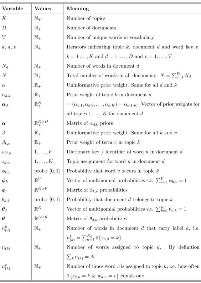
Figure 1: Graphical model: LDA
between the nodes in Figure 1 are as follows:
φk|β ∼ DirichletV(β) (1)
θd|α ∼ DirichletK(α) (2)
zd,n|θd ∼ CategoricalK(θd) (3)
wd,n|zd,n,φ ∼ CategoricalV(φzd,n) (4) For an overview of all notational definitions, refer to Table 1.
As mentioned before, LDA is a generative probabilistic model. This means that the observed words are assumed to be a result of underlying latent distributionsθ,φandz. How
exactly these distributions interact can be seen from the generative model:
1. For each topick= 1,2, . . . , K:
• Draw a distribution over words φk|β∼DirV(β) 2. For each document d= 1,2, . . . , D:
• Draw a topic mixture θd|α∼DirK(α)
• For each word n= 1,2, . . . , Nd in document d:
- Draw a word-topic assignment zd,n|θd∼ CatK(θd) - Draw a word wd,n|zd,n,φ∼CatV(φzd,n)
Note that the LDA setup thus far assumes scalar values for the hyperpriors α and β. In
such a setting the hyperpriors are uninformative. Alternatively, α and β may be
document-and/or topic-specific, respectively, making them informative. Extending to informative hy-perpriors, however, will be postponed to Section 3.
The joint probability of all latent variables (θ, φ, z) and observed variables (w) in the
p(θ,φ,z,w|α,β) = K Y k=1 p(φk|β) ! D Y d=1 p(θd|α) Nd Y n=1 p(zd,n|θd)p(wd,n|zd,n,φzd,n) (5)
The interest of LDA, however, only indirectly involves the joint probability, because the main goal is to find the posterior of the latent distributions:
p(θ,φ,z|w,α,β) = p(θ,φ,z,w|α,β)
p(w|α,β)
where the denominator requires integration over the full spaces of θ, φ and z. Even if an
analytical solution existed, execution would be prohibitively expensive. Therefore, exact in-ference is not an option at this point and focus must be shifted towardsapproximate inference. Two main types of approximate inference are used in the context of LDA: Collapsed Gibbs sampling (Section 2.2) and variational inference (Section 2.3).
Key to the success of LDA is the choice for the conditional distributions: neighbouring nodes in the graphical model are always conjugate pairs (Section 2.1). In other words, the parent nodes that serve as a prior to their child nodes result in very convenient posterior dis-tributions. This significantly eases the derivations of the conditional posterior disdis-tributions.. In Section 2.2 the collapsed Gibbs sampling approach by Griffiths and Steyvers (2004) for approximate inference will be introduced. Section 2.3 will start by introducing the concept of variational inference in general terms, including some necessary lemmata. Section 2.4 will then apply variational inference in the LDA setting.
2.1 Conjugate Priors
In the generative model, θdserves as a prior for the distribution of zd,n|θd. This section will demonstrate that using a Dirichlet distributed prior in a categorical distribution will lead to a Dirichlet distributed posterior. That is, the Dirichlet distribution is the conjugate prior of the categorical distribution. In order to do so, (2) and (3) will be formulated explicitly after which the distributions are combined to derive the distribution of the posterior and show conjugacy: p(θd|α) = Γ PK j=1αj QK j=1Γ(αj) K Y k=1 θαk−1 d,k (Dirichlet prior)
Extending the distribution ofzd,n in (3) toz yields: p(zd,n=k|θd) = K Y k=1 θ1{zd,n=k} d,k p(z|θ) = D Y d=1 Nd Y n=1 K Y k=1 θ1{zd,n=k} d,k (Categorical likelihood)
Using the Dirichlet prior as the parameter in the categorical likelihood results in a Dirichlet posterior: p(z|θ)·p(θ|α) = D Y d=1 Nd Y n=1 K Y k=1 θ1{zd,n=k} d,k Γ PK j=1αj QK j=1Γ(αj) | {z } =B(α) K Y k=1 θαk−1 d,k =B(α) D Y d=1 Nd Y n=1 K Y k=1 θ(αk−1)+1{zd,n=k} d,k =B(α) K Y k=1 θ (αk−1)+ D P d=1 Nd P n=1 1{zd,n=k} d,k ∝DirK(αk+ D X d=1 Nd X n=1 1{zd,n=k})
= DirK(αk+n(k)) (Dirichlet posterior) The posterior stems from the same distributional family as its prior, so conjugacy has been shown. The final expression classically shows how the posterior distribution is determined by both the prior α as well as the datan(k).
Analogously, the posterior of the prior-likelihood pair p(φzd,n|β) and p(wd,n|φzd,n) is
p(φ|β) = K Y k=1 p(φk|β) = K Y k=1 Γ(PV v=1βv) QV v=1Γ(βv) V Y v=1 φβv−1 k,v p(w|φ,z) = D Y d=1 Nd Y n=1 K Y k=1 V Y v=1 φ1{zd,n=k&wd,n=v} k,v
which results in the following Dirichlet posterior
p(w,φ|β)∝DirV βv+ D X d=1 Nd X n=1 K X k=1 1{zd,n=k&wd,n=v} = DirV(βv+nv(k))
2.2 Collapsed Gibbs Sampling
One way to deal with an unknown or complicated joint density like (5) is Markov chain Monte Carlo (henceforth MCMC), or more specifically (collapsed) Gibbs sampling (Geman and Geman, 1984). In MCMC, a Markov chain is constructed for which the equilibrium distribution has the properties of the target distribution. Repetitively resampling from this Markov chain is the essence of MCMC and will eventually result in a state from which samples are an asymptotically exact draw from the target distribution (Robert and Casella, 2005). Multiple rules have been developed by which the repetitive resampling is performed. One of these rules is called Gibbs sampling (Geman and Geman, 1984) in which the next state in the Markov chain is attained by sampling all variables, conditional on all other variables and the data. In other words, instances of every variable are sequentially drawn from their respectivefull conditional distributions.
Gibbs sampling is particularly useful when the target distribution is overly complicated, but its ’building blocks’ (i.e. full conditionals) are known and simpler. This method was first introduced in the context of LDA by Griffiths and Steyvers (2004) and has played a big part in the development of LDA extensions, including the extensions presented in this thesis.
In order to get the full conditionals in the LDA framework, one needs to know the expected value of a Dirichlet distributed random variable:
Lemma 1 (Expected value of Dirichlet). Letµ∼DirJ(α) then E[µk] = PJαk j=1αj
.
As outlined in Griffiths and Steyvers (2004), only the topic-word assignments zd,n are sampled. Hence the full conditional of interest is
p(zi =k|z−i,w) (6)
where the subscript −i indicates that all values except the i-th value are considered. This
probability distribution describes the probability that a given wordwiwill be assigned to topic
k, given that all datawand all other word-topic assignmentsz−i are known. For notational convenience, the subscript referring to document das well as explicitly conditioning on the
hyperpriors α and β have been dropped. The difference in notation will be emphasised by
introducing the subscript i, which will temporarily replace the subscript (d, n). By the end
of the derivation, the usual notation will return and the result will be transformed to reflect document membership again.
Most terms that rely on available data w or terms that are part of the conditioning
dimensions of the distributions, while only affecting the characteristics of the distribution up to a multiplicative constant. p(zi =k|z−i,w) = p(zi =k, wi|z−i,w−i)·p(z−i,w−i) p(z−i,w) ∝p(zi =k, wi|z−i,w−i) =p(wi|zi=k,w−i,z−i)·p(zi =k|w−i,z−i) =p(wi|zi=k,w−i,z−i) | {z } =CGS: Term 1 ·p(zi=k|z−i) | {z } =CGS: Term 2 (CGS: all terms) The full conditional has been split in two distributions. The first may be interpreted as the probability that a word wi is drawn, given that the word has been assigned to topic k. The second probability is broadly interpretable as the relative frequency of topic k in the entire
corpus.
• CGS: Term 1. Further investigation of the first term leads to p(wi|zi =k,w−i,z−i) = Z p(wi|zi =k,φk) | {z } =φk,wi ·p(φk|z−i,w−i) | {z } see (8) dφk (7)
The second part of the integrand can be reformulated to a conjugate likelihood-prior structure for which the resulting posterior has been derived in Section 2.1
p(φk|z−i,w−i) =
p(w−i,φk|z−i)·p(z−i)
p(z−i,w−i)
∝p(w−i|φk,z−i)·p(φk)
= DirV(nv−i,(k)+β) (8) The expression in (7) is therefore equal to the expected value of a Dirichlet distributed random variable. Using Lemma 1, the first term in (CGS: all terms) is equal to
p(wi|zi =k,w−i,z−i) = nwi −i,(k)+β P j6=i nwj −i,(k)+β = n wi −i,(k)+β n−i,(k)+V β (CGS: Term 1) • CGS: Term 2. Analogous reasoning will be applied to the second term:
p(zi =k|z−i) = Z p(zi=k|θd) | {z } θd,k ·p(θd|z−i) | {z } see (10) dθd (9)
The second part of the integrand can be reformulated as a conjugate likelihood-prior pair for which the posterior is known from Section 2.1
p(θd|z−i) =
p(z−i|θd)·p(θd)
p(z−i)
∝p(z−i|θd)·p(θd)
= DirK(nk−i,(d)+α) (10) Hence (9) is the expectation of a Dirichlet distributed random variable, which is the final expression for the second term in (CGS: all terms)
p(zi =k|z−i) =
nk−i,(d)+α
n−i,(d)+Kα (CGS: Term 2) Inserting (CGS: Term 1) and (CGS: Term 2) into (CGS: all terms) yields the full condi-tional that was first formulated in Griffiths and Steyvers (2004):
p(zi =k|z−i,w) = nwi −i,(k)+β n−i,(k)+V β · n k −i,(d)+α n−i,(d)+Kα (11) Intuitively, this may be interpreted as the product of two empirical probabilities: The probability that wordwi occurs in topickmultiplied by the probability hat topickoccurs in document d. This expression will play a major role in the dynamics of the LDA extensions
in this paper.
At this point, the rule by which samples are repetitively drawn in the Monte Carlo procedure has been established: every draw is performed on the full conditional. The full conditional of every zi is dependent on z−i so the rule must constantly be adapted to the current state of the Markov chain. Once all zi are assigned a value between 1 and K, the Markov chain is initialised, the iterative sampling procedure according to the ever-changing full conditional distribution of thezi’s can be started.
A sample from the posterior distribution p(z|w) is generated in every iteration of the
Markov chain. Latent distributions φ and θ can be estimated from every one of these
iterations: ˆ φk,v = nv(k)+β n(k)+V β ˆ θd,k= nk(d)+α n(d)+Kα
After a burn-in period of iterations, everyt-th sample (Markov state) can be saved. Taking
over new words w and topics z conditioned on w and z" (Griffiths and Steyvers, 2004,
p. 5230).
So far the collapsed aspect of this Gibbs sampling procedure has not been addressed ex-plicitly. The document-topic distributionθand topic-word distributionsφserve as (Dirichlet)
priors to the categorical likelihood z. As can be seen in equations (7) and (9), these priors
have been integrated (collapsed) out. The collapsing out results in an unconditional distri-bution (independent of its prior) from which samples will be taken. In case of conjugate pairs, the resulting distribution has a particularly simple form in comparison to the initial conditional distributions, thus making the Gibbs sampling process less complex. Also, de-pendencies between all categorical variables that relied on the Dirichlet prior are created. This can be easily confirmed by observing that the distribution ofzi is partially determined by z−i via then-terms in (11).
2.3 Variational Inference: Background
The posterior distribution of all latent distributionsp(θ,φ,z|w,α,β) is to be computed, but
is intractable. Variational inference can be used to deal with models for which it is infeasible to evaluate the posterior distribution. Infeasibility may stem from the high dimensionality of latent spaces or complex forms that disable analytical tractability (Bishop, 2006, p. 461). By using the tools of variational inference, the posterior distribution can be approximated by more handleable distributions that in turn can be optimised. The general idea is to minimise the Kullback-Leibler divergence (Kullback and Leibler, 1951) between the true posterior and the approximate distribution, whilst restricting the family of distributions from which we can select the approximate distribution. The family must be rich enough to resemble relevant features of the true distribution, while simultaneously be restricted to family members that are tractable and feasible for optimisation.
Assume a model with observed variables xand latent variablesysuch that the posterior
distributionp(y|x) is intractable, due the high dimensionality of the latent space in whichx
resides. The aim of variational inference is to approximate p(y|x) with a tractable density q(y). To do so, the Kullback-Leibler divergence is minimised
q∗(y) = arg min
where KL (q(y)||p(y|x)) = Eq log q(y) p(y|x)
= Eq[logq(y)]−Eq[logp(y|x)] = Eq[logq(y)]−Eq[logp(y,x)] +logp(x)
and where D is the family of distributions from which we can select q(y). The above still
involves p(x), however it is nothing more than an additive constant in the optimisation
function (12), so it may be ignored.
Since the KL-divergence is non-negative (Kullback and Leibler, 1951), it is easy to verify that logp(x) is lower bounded by Eq[logp(y,x)]−Eq[logq(y)]. Because logp(x) is also referred to as the evidence in Bayesian statistics, the following is called Evidence Lower Bound (ELBO):
ELBO(q) = Eq[logp(y,x)]−Eq[logq(y)] (13) From the definition of the KL-divergence and ELBO(q), it can be seen that minimising the
KL-divergence w.r.t. q(y) is equivalent to maximising ELBO(q) which is what the focus will
be on henceforth.
If no restrictions are placed on the family of distributions D from which q(y) can be
selected, the optimal choice would be to setq(y) equal top(y|x), because the KL-divergence
would obviously be zero. To ensure simplicity in the structure of the variational distribution,
q(y) is limited to distributions that factorise over all its marginal distributions. In other
words, the joint variational distribution ofy= (y1, y2, . . . , yM) is equal to the product of the marginal variational distributions
q(y) =
M
Y
m=1
qm(ym)
This is known as the mean-field variational family, where each latent variable is represented by its own variational factorqm(ym), that may be considered as factorised marginal distributions (Blei et al., 2017; Jordan et al., 1999).
In general, a joint distribution p(x,y) (such as the one in (13)) can be factorised like
logp(y,x) = log " p(x) M Y m=1 p(ym|y−m,x) # = logp(x) + M X m=1 logp(ym|y−m,x) Incorporating the mean-field variational family assumption in ELBO(q) now yields
ELBO(q) = logp(x) +
M
X
m=1
Recall that the aim is to maximise ELBO(q) with respect to the variational distributions,
hence logp(x) may be regarded as a constant. Since the ELBO(q) will be maximised and
eventually the derivative w.r.t. qm(ym) will be set to zero, a convenient formulation makes all dependencies on qm(ym) explicit. Using the law of iterated expectations, taking the partial derivative and solving forqm(ym) yields
ELBO(q)m= Z qm(ym) E−m[logp(ym|y−m,x)]dym− Z qm(ym) logqm(ym)dym ∂ELBO(q)m ∂qm(ym) = E −m[logp(ym|y−m,x)]−logqm(ym)−1= 0! qm∗(ym)∝exp [E−m(logp(ym|y−m,x))] (14) This expression can be solved when p(ym|y−m,x) has been derived, which will be done in Section 2.4.
Before moving on to the general solutions for exponential family members, it is interesting to pay close attention to the similarities between Gibbs sampling and (coordinate ascent) variational inference. They are more closely related than one may suspect at first sight. Recall that Gibbs sampling uses the full conditional distribution to sample from. The coordinate ascent variational inference method discussed here uses the (exponentiated) expected (log) value of that full conditional (see (14)) to set each variational factor (Blei et al., 2017).
In addition to (14), there is another useful relation between the optimal variational factors
qm∗(ym) and the full conditionals. If the full conditional is a member of the exponential family, then qm∗(ym) is member of that same family, but with different natural parameters νm∗ (see Appendix A for a proof). The only difference (up to a multiplicative constant) between the true full conditionals and the variational factorsqm(ym) lies in the natural parameters, which is the reason why in this setting they are also referred to as the variational parameters of
qm(ym):
νm∗ ∝Eq−m[ηm(x,y−m)] (15) whereηm(x,y−m) is the natural parameter of the complete conditional. For a full derivation, refer to Appendix A.
In order to arrive at the variational factors in the LDA model, it is useful to be aware of the following lemmata:
Lemma 2(Markov blankets). LDA is a statistical model that can be expressed as a graphical
model (see Figure 1). Such Bayesian networks posses a number of properties that help in identifying conditional independence of nodes in the network. Awareness of these properties
allows one to nimbly assess whether the conditioning set of variables can be reduced or not, without affecting the conditional distribution. The Markov blanket of a nodeA- denoted as M B(A) - in a Bayesian network consists of
1. all parents ofA
2. all children of Aand
3. all parents of the children ofA (so called co-parents ofA).
All nodes outside of M B(A) are conditionally independent of A if conditioned on M B(A).
This implies that all nodes outside ofA’s Markov Blanket are redundant in the conditioning
set as long asM B(A) is contained in the conditioning set (Bishop, 2006).
Lemma 3(D-separation due to collider node). A path between nodesAandC in a Bayesian
network is d-separated (i.e. blocked) by a node set Z if both nodes A and C are directed
towards B, and neither B nor any of its descendants are part of the set Z (Geiger et al.,
1990).
Lemma 4 (Expected value of log-Dirichlet). Let x ∼ DirJ(α), then the expected value of
the logarithm ofxk equals
E(logxk) =ψ(αk)−ψ J X j=1 αj
whereψ(y) = dyd log Γ(y) is the digamma function.
Lemma 5 (Natural parameters - Dirichlet distribution). Letx∈RM and x∼Dir(α), then the natural parameter ofx is
η(x,α) = (α1, . . . , αM)
Lemma 6 (Natural parameters - categorical distribution). Let x ∈ {1, . . . , N} and x ∼
CatN(p), then the natural parameter ofx is
η(x,p) = (logp1,logp2, . . . ,logpN) 2.4 Variational Inference in Latent Dirichlet Allocation
In order to use (15) and obtain the optimal variational parameters, the full conditionals of the latent distributions are required. Three groups of latent distributions exist in LDA:z,φ
with obtaining the true full conditionals (Section 2.4.1) and will afterwards proceed with the identification of the optimal variational distributions (Section 2.4.2). As a final result, we will end up with the Coordinate Ascent Variational Inference (CAVI) algorithm for LDA.
2.4.1 Full Conditionals in LDA
Getting to the full conditionals will build on the conjugacy results of Section 2.1 and on the lemmata presented at the end of Section 2.3.
1. Full conditional of document-topic distributions: The Markov blanket M B(θd) consists of the parents α and the childrenzd(there are no co-parents forθd), so
p(θd|z,θ−d,φ,w) =p(θd|zd, α) where it is known that zd ∼ QNd
n=1Cat(θd) and θd|α ∼ Dir(α) from the LDA model specification. By the conjugacy results from Section 2.1, the full conditional of topic proportions p(θd|zd, α)∼Dir(α∗d), where
α∗d= α+ Nd X n=1 1{zd,n= 1}, . . . , α+ Nd X n=1 1{zd,n=K} (16) = α+n1(d), . . . , α+nK(d)
2. Full conditional of topic-words distributions: The Markov blanketM B(φk) con-sists of the children z, the co-parents φ−k and w, and parents β, so
p(φk|z,θ,φ−k,w, β) =p(φk|z,φ−k,w, β)
∝p(φk,w|z,φ−k, β)
=p(w|φk,φ−k,z, β)·p(φk|φ−k,z, β) =p(w|φ,z)·p(φk|β)
where the last term in the final equation follows from Lemma 3: wd,n is the colliding node betweenφk andz, butwd,nis not part of the conditioning set and therefore they are conditionally independent. From the LDA model specification it is known that
p(w|φ,z) ∼QD
d=1
QNd
n=1Cat(φzd,n) and p(φk|β) ∼Dir(β). Considering that the latter serves as a conjugate prior to the former distribution, it is known (see Section 2.1) that the result must follow a Dir(β∗k) distribution, where
βk∗= β+ D X Nd X 1{zd,n=k&wd,n=1} , . . . , β+ D X Nd X 1{zd,n=k&wd,n=V} (17)
3. Full conditional of word assignments: The Markov blanket M B(zd,n) consists of the parentsθd, the children wd,n and the co-parentsφk. Hence
p(zd,n=k|z−d,n,θ,φ,w) =p(zd,n=k|θd,φk, wd,n)
This is a conditional distribution that is not known directly, but using the chain rule the above equation can be written like
p(zd,n=k|θd,φ, wd,n)∝p(zd,n=k, wd,n=v|θd,φ)
=p(wd,n=v|zd,n,θd,φzd,n)·p(zd,n=k|θd,φ) =p(wd,n=v|zd,n,φ)·p(zd,n=k|θd)
=φk,v·θd,k (18)
whereθdis cancelled because it is not part of theM B(wd,n) andφis cancelled because it is d-separated from zd,n by the node wd,n (Lemma 3)
2.4.2 Variational Factors in LDA
With the results from the previous section, we now know the distributional family of each vari-ational factor, but the parameters for those distributions are still unknown. Let the unknown parameters be γd, λk and ψd,n for the document-topic, topic-word and word-assignment distributions, respectively:
1. Variational distribution of document-topic distribution: qθd(θd) = Dir(γd). The natural parameters,ηθd(α,zd), of the full conditional are (α+n
k
(d)) fork= 1, . . . , K.
2. Variational distribution of topic-word distribution: qφk(φk) = Dir(λk). The natural parameters, ηφk(β,zd,n), of the full conditional are β +
PD
d=1
PN
n=11{zd,n=k&wd,n=v} forv= 1, . . . , V.
3. Variational distribution of word assignment distribution: qzd,n(zd,n) = Cat(ψd,n). By Lemma 6, the natural parameters,ηzd,n(φzd,n,θd, wd,n), of the full conditional are equal to the logarithm of the parameters. Thereforeηzd,n(φzd,n,θd, wd,n) = logφk,vlogθd,kfor
k= 1,2, . . . , K.
The natural parameters of the full conditionals will be crucial in this section, since they have been linked explicitly with the optimal natural parameters of the variational factors (see expression (15)).
1. Variational distribution of document-topic distributions: To find the
appropri-ate parametersγdfor the variational distribution, we will rely on (15):
γd∗ ∝Eq−γd[ηθd(α,zd)]
The reasonαandzdappear in the expression is that they constitute the Markov blanket that was used in the full conditional.
The expectation is taken w.r.t. all variational distributions, exceptγd. Since the term inside the expectation operator, i.e. the natural parameters of the full conditional, contains onlyα and zd, the expected value is equivalent to Ezd[ηθd(α,zd)]. We have
γd,k∗ ∝Eqzd,k[ηθd,k(α,zd)] =α+ Nd X n=1 Eqzd(1{zd,n=k}) =α+ Nd X n=1 ψd,n,k
where the final line follows from the fact thatqzd follows a categorical distribution with the (unknown) parameters ψd,n,k for n= 1, . . . , Nd and k= 1, . . . , K. The document-topic variational distribution isqθ∗
d,k = Dir(γ
∗
d,k).
2. Variational distribution of topic-words distributions: Analogous to the
deriva-tion for the variaderiva-tional distribuderiva-tion of the document-topic distribuderiva-tions, we know that
λ∗k,v ∝Eq−λ k(ηφk(β, zd,n)) = Eqzd,n(ηφk(β,z)) = β+ D X d=1 Nd X n=1 Eqzd,n[1zd,n=k]1wd,n=v = β+ D X d=1 Nd X n=1 ψd,n,k·1wd,n=v
Therefore, the variational distribution of the topic-words distributions isq∗φ
k,v = Dir(λ
∗
k,v). 3. Variational distribution of word assignments: By expression (16), the natural
parameters of the variational distribution of zd,n are
νq∗zd,n ∝E−ψd,n[ηzd,n(φzd,n,θd, wd,n)]
Sinceqzd,n(ψd,n) is a categorical distribution, the natural parameters are the logarithm of the parameters (see Lemma 6). The actual parameters ofq (ψ ) are denoted as
ψd,n: ψd,n,k∗ = expνq∗ zd,n ∝expE−ψd,n[ηzd,n(φzd,n,θd, wd,n)] = exp E−ψd,n[logφk,v+ logθd,k] = exp Eqφk[logφk,v] + Eqθd[logθd,k] = exp Ψ(λk,v)−Ψ( V X u=1 λk,u) + Ψ(γd,k)−Ψ( K X j=1 γd,j)
where the last line follows from Lemma 4.
3 Incorporating Available Information
The input required to perform baseline LDA is merely a corpus with documents, the number of topics K and a value for the hyperpriors α and β. The corpus used in this paper has
an additional source of information that can be exploited, namely the JEL codes for each document. Not only are the documents labeled, the structure of the labels is also known. For example, the labels D12and D01are both members of the label family Dand are likely to have more in common than labelsA14 andQ21. By incorporating such prior knowledge, the unsupervised baseline LDA can be transformed into a (semi)supervised method.
This section will present three extensions to the baseline LDA model: Labeled LDA (L-LDA), Hierarchically Supervised LDA (HSLDA) and CascadeLDA. Each of the extensions utilises the available information in its own way and the quality of their results depends on the ultimate aim of the user and at times on very specific features of the dataset.
3.1 Extension 1: Labeled LDA
The aim of this paper is to build a classifier that is able to recommend JEL codes for previously unseen academic abstracts and full academic papers. This implies that the interest is not to identify latent topics, but rather explicit topics that have a one-to-one correspondence with the JEL codes. There are multiple ways to manipulate the topics identified by LDA. One could, for example, provide a set of seed words and use them to bias topic-word distributions towards certain terms (Jagarlamudi et al., 2012). Alternatively, by creating Must-Links and Cannot-Links between words and topics (Andrzejewski et al., 2009) the structure of topic-word distributions is restricted in a favourable way. These methods can be used if the dataset is an unlabeled corpus, but the researchers have some domain knowledge about the topics they wish to identify. External knowledge sources such as Wikipedia articles regarding the
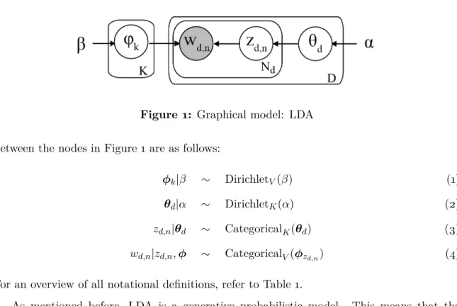
Figure 2: Graphical model: Labeled LDA
desired topics can also be used as a form of prior knowledge (Wood et al., 2016). In the case of this research, we can manipulate the topics to exactly correspond with the labels. Such a setting of explicit topics in labeled data has been investigated in Ramage et al. (2009) and Rubin et al. (2012). A crucial piece of information is that the topics/labels covered in a every document is known a priori and more importantly, it is known which topics are not part of the document. To put the above in more LDA-specific terms: It is known which of theK elements inθd have a positive document-topic mixture and which elements are equal to zero. Hence, the space in which the topic-document distribution resides (during training) for every document can be shrunk tremendously, since it is limited to only the JEL-codes attached to that document. This causes a shift in the way the conditional distributions in the model interact through a three step process: Firstly, the parameters for the distribution ofzd,n (recall thatzd,n∼CatK(θd)) are mostly equal to zero, with positive values only in the positions that correspond to the labels of the document. This leads to the second step of the process: zd,1:N can only be assigned to the positively loaded labels, hence all wordswd,1:N
in that document will be associated with those labels. As a result, document d only affects
those topic-word distributions φk that correspond to the topics (labels) of that document. The above has been dubbed Labeled LDA or L-LDA by Ramage et al. (2009), who claims that L-LDA outperforms support vector machines in identifying label-specific docu-ment snippets and is competitive when it comes to discriminatively assigning labels to unseen documents. Despite some contextual differences, L-LDA is in practice equivalent to Rubin’s Flat-LDA (Rubin et al., 2012).
Figure 2 illustrates how the label information is incorporated to extend the baseline LDA model. The full generative model of L-LDA is nearly identical to LDA, except for the document-topic distribution θd:
θd ∼ DirK(α·Ωd)
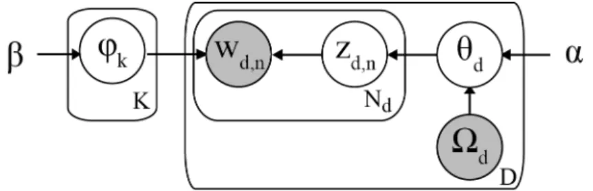
Table 2: The ten most likely words for five JEL codes
root E32 D82 J24 R31 I12
econom cycl agent skill hous mortal
cours model inform capit price health
signific busi princip human boom increase
student shock optim educ transact percent
research recess mechan labor home age
author aggreg privat school area birth
regress volatil effici worker buyer suggest
expeditur rate incent occup percent rate
call fluctuat alloc wage seller life
yield product select college rent effect
rootis the generic label that is assigned to all documents to improve classification results of real labels E32: Macroeconomics & Monetary Economics → Prices, Business Fluctuations & Cycles → Business Fluctuations - Cycles
D82: Microeconomics → Information, Knowledge & Uncertainty → Asymmetric & Private Information -Mechanism Design
J24: Labour & Demographic Economics → Demand & Supply of Labour → Human Capital Skills -Occupational Choice - Labour Productivity
R31: Urban, Rural, Regional, Real Estate & Transportation Economics → Real Estate Markets, Spatial Production Analysis & Firm Location →Housing Supply and Markets
I12: Health, Education & Welfare → Health → Health Behaviour
d’s label set. This is the dynamic that forces all topic-loadings that are not part of the
document’s label set to zero while keeping the rest positive. It results in highly accurate topic-word distributions for each label as can be seen in Table 2.
An important characteristic is therootlabel which is assigned to every single document. The purpose of this label is to capture generic (academic) language and thus clean these words from the actual JEL labels.
Shrinking a document’s topic-document distribution sets the stage for a noteworthy side effect. Due to the fewer possible values, the iterative processes of Gibbs sampling and CAVI during training time converge much faster and in a more stable way.
3.2 Extension 2: Hierarchically Supervised LDA
The labels of the documents have an implicit structure which is illustrated in Figure 3. The labels consist of one letter and two digits, like D42 and F31, where the letter stands for a general category (level 1) such as microeconomics or international finance. The first digit represents the first refinement within the general category (level 2) and the second digit provides the final level of granularity (level 3 or leaf label). Therefore, it is to be expected that JEL codeD421has a topic-word distribution very closely related to the JEL code D412. More generally, neighbouring leaf labels tend to be highly similar and are, also for the human reader, hard to distinguish between.
The idea of related topics within the LDA model has been investigated in a number of papers (e.g. Blei and Lafferty (2006)), but these generally do not allow for pre-specified correlations between the topics, whereas our dataset would require so. Additionally, the Semi-Supervised Hierarchical Topic Model (SSHLDA) by Mao et al. (2012) introduces a promising model which learns new topics automatically. Since the aim of this thesis is to classify according to pre-specified label and not to identify new topics, SSHLDA would unnecessarily complicate computations and derivations in this thesis, without any guarantee regarding the correctness of the hierarchy. Dependency-LDA introduced by Rubin et al. (2012) does account for dependencies between labels while also allowing for multiple labels per document. However, Dependency-LDA would require creating positive loadings to all of the topics that are related to the document’s labels which in turn decreases the discriminative power of the model. Additionally, it is specifically designed to perform well on corpora with a large number of labels whose frequencies follow a power law distribution. Since Dependency-LDA outperforms other methods only for datasets with labels that follow a power law distribution, this method has also not been pursued further.
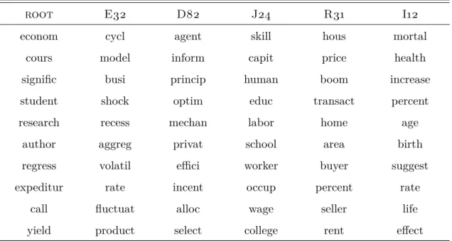
Another promising model is found in Hierarchically Supervised LDA (HSLDA) by Perotte et al. (2011) for which performing out-of-sample predictions is the primary aim. The base-line LDA model is augmented with an entirely new mechanism that exploits the hierarchy structure of the labels viazd,n. Figure 4 shows the graphical model for HSLDA. The top part of the model is a baseline LDA model in which actual latent topics are searched for. The information on the document labels is integrated in the bottom part of the graphical model.
1D42: Microeconomics → Market structure, pricing → Monopoly
Figure 3: Label structure: JEL code tree 3.2.1 Generative Model
Before diving into the technical parts, a more intuitive explanation of the model’s mechanics will be provided here. The most intuitive take on this model is to start off at node aroot,d. This node serves as a running variable in a probit model and follows a normal distribution with mean ¯z1ηroot,1+¯z2ηroot,2+· · ·+¯zKηroot,K, where ¯zkrepresents the current share of topick in the document-topic mixture. During testing a given label will be assigned to a document only if its corresponding running variable exceeds a pre-specified threshold. If that is the case, the label dummy yl,d for label l is set to one. The running variables further down the label tree are dependent on the other label dummies. During testing they are truncated from above at the threshold if its parent has a value below the threshold. It is therefore impossible for a label down the label tree to turn positive when any of its ancestors is negative. As all labels are known during training time, the running variables are always forced either below or above the threshold. By doing so, the regression coefficients ηl,k are trained to reflect the interaction between the observed labels and the latent topics identified in the top part of the graphical model.
Note that the top part that identifies latent topics is not the actual aim of this model. The crucial aspect are the running variables and the label dummies: the latent topics are merely a tool to help achieve that goal.
Figure 4: Graphical model: Hierarchically Supervised LDA
Except for the specification ofαandβ3, this generative model corresponds to the original
HSLDA:
1. For each topick= 1, . . . , K
• Draw a distribution over words φk|β∼DirV(β) 2. For each label l∈ L
• Draw a label application coefficient ηl|µ,σ∼ NK(µ,σ), where µ containsK identical values andσ = diag(σ) for σ >0..
3. For each document d= 1, . . . , D
• Draw topic proportions θd|α∼DirK(α) • Forn= 1, . . . , Nd
- Draw a word assignment zd,n|θd∼CatK(θd) - Draw a word wd,n|zd,n,φ∼CatV(φzd,n) • Set the root node yroot,d= 1
• For each label linL, starting at the children ofroot
3The original prior structure uses Hierarchical Dirichlet Priors (HDP). Due to its complex construct and a
- Drawal,d|z¯d,ηl, ypa(l),d∼ N(z¯dTηl,1), ifypa(l),d= 1 N(z¯dTηl,1)1{al,d<0}, ifypa(l),d=−1 - Apply labell to documentdaccording to
yl,d|al,d= 1 ifal,d >0 −1 else
wherez¯dT = (¯z1, . . . ,z¯K) are the fractions of words that are assigned to topickin document
d, i.e. ¯z1 = N1
d
PNd
n=11{zd,n=k}. This may be regarded as an intermediate estimate ofθd. The hierarchical coupling of the regression coefficients ηl creates a posteriori dependence which causes label predictors deeper in the hierarchy to focus on distinguishing features between a label’s levels.
3.2.2 Gibbs Sampling
Collapsed Gibbs sampling is used for approximate inference in HSLDA. Whereas the baseline LDA model collapsed out all latent variables except zd,n, HSLDA involves two additional latent conditional distributions, namelyal,d and ηl.
• The conditional posterior distribution of the words’ topic assignmentszd,n used in this
paper differs in some important ways from the original HSLDA specifications. Instead of conditioning on the running variables a, we will condition ony. The reason for this
is discussed a bit further below. This leads to
p(zd,n|z−d,n,y,w,η, α, β) = p(y, zd,n|z−d,n,w,η, α, β)·p(z−d,n,w,η, α, β) p(z−d,n,y,w,η, α, β) ∝p(yd, zd,n|z−d,n,w,η, α, β) =p(yd|zd,n,z−d,n,w,η, α, β)·p(zd,n|z−d,n,w,η, α, β) =p(yd|z,η)·p(zd,n|z−d,n,w, α, β)
where the conditioning sets of both terms could be reduced in the final line, because those nodes are outside the relevant Markov blanket (Lemma 2), and zd,n and η are d-separated by al,d (Lemma 3). Considering that the variables in yd can only take
values in {0,1}, we know that p(yd|z,η) = Y l∈Ld p(yl,d = 1|z,η)yl,d·p(yl,d= 0|z,η)1−yl,d = Y l∈Ld p(al,d> c|z,η)yl,d·p(al,d< c|z,η)1−yl,d = Y l∈Ld Z ∞ c exp −1 2(¯zTdηl−al,d)2 dal,d · Y j /∈Ld Z c −∞exp −1 2(¯zTdηj−aj,d)2 daj,d (19)
This derivation differs in two ways from the original HSLDA formulation. Firstly, the original HSLDA takes only the product for present labels into account, thus effectively ignoring the second term. This is justified by the assumption that absent labels may actually be part of the document’s true label set as opposed to its observed label set, so the absent labels are not restricted to be below the threshold. This implies that the second set of integrals in (19) are evaluated from −∞ to ∞. Since these integrals are
proportional to probability density functions, they can be ignored. For the corpora in this thesis, however, it is implicitly assumed that the labels assigned to a document indicate that paper’s true present (positive) labels, and therefore also its absent (nega-tive) labels. Secondly, this paper focuses onp(yl,d|z,η) (i.e. the conditional probability thatal,d is larger or smaller than threshold c) instead of p(al,d|z,η). The reason being that the former quantifies the distance from the threshold better than the latter and thus also captures the "magnitude of presence" more accurately.
The second term in (19) is equivalent to the results in Section 2.2 (Eq. 11):
p(zd,n|z−d,n,w, α, β) = nwi −i,(k)+β n−i,(k)+V β · n k −i,(d)+α n−i,(d)+Kα
• The conditional posterior distribution of the regression coefficients ηl corresponds to
the least squares regression results with priors µ and σ conditional on the available
data. In the statistics literature, this is referred to as a ridge regression:
p(ηl|z,a, µ, σ) =N( ˆµl,Σˆ) where ˆ µ= ˆΣ 1µ σ + ¯ ZTal and Σˆ−1 =IKσ−1+ ¯ZTZ¯
• The conditional posterior distribution of the running variablesal,d is closely related to the model specification fora |¯z ,η, y . The difference is that the probability is
Figure 5: Graphical model: CascadeLDA
forced to zero (truncated) if the is-a hierarchy between yl,d and al,d is violated. This results in p(al,d|z,Y,η)∝ exp{−12(¯zTdηl−al,d)2}1{al,dyl,d>0} ifypa(l),d= 1 exp{−12(¯zTdηl−al,d)2}1{al,dyl,d>0}1{al,d<0} ifypa(l),d=−1 3.3 Extension 3: CascadeLDA
CascadeLDA is designed to take advantage of the hierarchy structure in the labels with a different approach from the HSLDA mechanism. A foreseeable issue with the previously discussed extensions is that it seems unlikely for the topic-word distributions φk to be dis-criminative between sibling labels. By focusing on the entire corpus -or global scope- the topic-word distributions of leaf labels are bound to be polluted by the same dominant words that dominate their siblings’ (and parents’) topic-word distributions. On the one hand, this does represent that leaf label’s topic-word distribution, but on the other hand it does not help us in discriminating between sibling labels. CascadeLDA aims at finding discriminating features between sibling nodes by zooming in on a single (non-leaf) label at a time. The local scope then serves as a magnifying glass for the differences between sibling nodes.
Before proceeding, it is useful to be clear about the terminology used to explain Cas-cadeLDA. Firstly, the terms sibling label and neighbour label may be used interchangeably. Secondly, leaf labels are not necessarily level 3 labels. As the name suggests, it refers to the most detailed labels in the label tree. If the model ignores the level 3 labels, then the level 2 automatically become the leaf labels. Thirdly, all labels with descendants (i.e. all non-leaf labels) can serve as parent labels. Similarly, all labels except the root-label can serve as
child labels. Fourthly, each non-leaf label serves as the basis for a local scope. A local scope may also be referred to as neighbourhood or family scope.
The idea of CascadeLDA is to train an ensemble of L-LDA models in different local scopes. Each non-leaf label serves as a starting point of a local scope once during training time. This non-leaf label is called the parent label for that scope. All documents that have the parent label in their label sets are retained in the local scope, whereas all other documents fall outside the scope. For the retained documents the label sets are obfuscated to only contain the parent’s children labels (i.e the labels that descent from the parent label in Figure 3). The remaining documents and labels are referred to as subcorpus. After creating the subcorpus, L-LDA is performed on it. As a final, but crucial, manipulation of the subcorpus, a generic label is added to each document’s label set in addition to the children labels. This is the local scope analog of theroot-label.
Upon discarding all non-child labels, all non-family features of a document will be assigned to the generic label during training. In fact, all features shared by the documents in the subcorpus are assigned to the generic label. This includes generic parent label features. The only parts of a document that are likely to be attributed to the children labels are the ones that set a child label apart from its siblings.
After the L-LDA model in a local scope converged, the resulting topic-word distributions for the children labels are retained in the CascadeLDA model. Typically, CascadeLDA will then cascade down the label tree and choose one of the former child labels as the next parent label. This process is continued until all non-leaf labels have served as a parent label. After cascading down all branches, the CascadeLDA should have the topic-word distributions that distinguish sibling labels from each other.
In the classic L-LDA approach only leaf labels are considered labels. That is, no topic-word distribution is identified for e.g. the non-leaf label D8. In CascadeLDA, however, all non-leaf labels also have their own topic-word distributions. It may seem like a small detail, but leads to an important characteristic of CascadeLDA, because the topic-word distributions areonlyvalid (i.e. usable) in their respective scope. A discriminating feature in a local scope may very well be completely uninformative in the global scope. To see why, consider a human family in which the children are recognised based on their hair colour. Even though this may help in their family home, it will not suffice to identify the children outside the family setting. This creates a challenge during testing time: in which scope should an unseen document be tested? The process of testing starts at the root and attempts to assign the document to
one or more level 1 labels, in the same way L-LDA is applied for classification. After this, the testing procedure cascades down to each of the promising level 1 labels and the document’s content is fitted to that parent label’s local scope to discriminate between its children labels. This procedure is continued until all promising branches are pursued. A discussion on which labels are considered ’promising’ is postponed to Section 5.1.
Beware of certain dynamics that should be handled with caution. Consider the situation in which the words for a test document are convincingly assigned to e.g. labelB. As a result, the model will zoom in on labelBand make it the parent in the following local scope. Here it may occur that the test document does not contain any features that allow for recognition of B’s children, even though the document really is a member of theB-family. As a result, all words in the test document are assigned to the generic label and no further paths are considered in this branch and the prediction strands at a non-leaf label. For the datasets we are using this is not a favourable characteristic, because only leaf labels are assigned to documents.
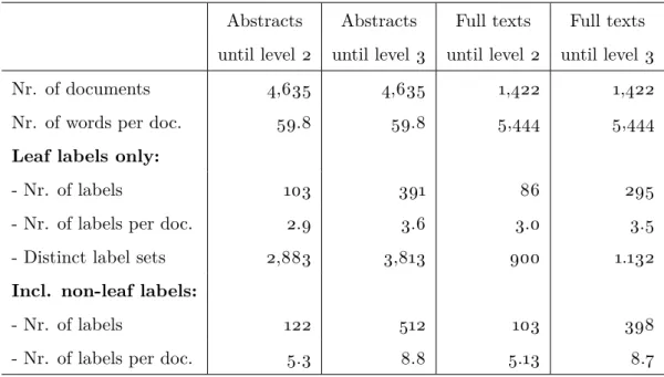
4 Data and Preprocessing
Two corpora containing JEL-labeled, academic texts are at our disposal to which the methods discussed are applied.
The first corpus consists of 4,635 abstracts that each contain an average of 60 (standard deviation: 18.9) unique tokens. In order to obtain a wide range of topics, the abstracts were gathered from different journals including American Economic Journals with the speciali-sation journalsApplied Economics,Economic Policy,Macroeconomics and Microeconomics. The creator of the JEL codes, the Journal of Economic Literature, is also the source of nu-merous abstracts in this research. Thus, the corpus should constitute a representative sample of the relevant academic economic literature of the past 20 years.
The other corpus is a collection of 1,422 full-text academic articles. Approximately half of the articles correspond to the same documents as the first corpus. The other half stems from theCollaborative Research Center 649: Economic Risk which is part of the interdisciplinary Center for Applied Statistics and Economics. All full-text articles have been gathered as PDF documents. After extracting the text from the documents all tables, images and non-text data has been removed.4 The documents contain on average 5,444 unique words (standard
Abstracts Abstracts Full texts Full texts until level 2 until level 3 until level 2 until level 3
Nr. of documents 4,635 4,635 1,422 1,422
Nr. of words per doc. 59.8 59.8 5,444 5,444
Leaf labels only:
- Nr. of labels 103 391 86 295
- Nr. of labels per doc. 2.9 3.6 3.0 3.5
- Distinct label sets 2,883 3,813 900 1.132
Incl. non-leaf labels:
- Nr. of labels 122 512 103 398
- Nr. of labels per doc. 5.3 8.8 5.13 8.7
Table 3: Summary statistics of the corpora
deviation: 2,228).
After training the classification models, the next step is to test and evaluate its effec-tiveness. As is standard in classification problems, the model will be applied to unseen documents, also known as the test set. Even though labels are available for the test set -making them theoretically suitable to use for training - all documents in the test set have been isolated from the model during training. Failing to strictly split training data from test data is likely to lead to overfitting and the external validity of the classification would immediately be compromised.
The documents are labeled by humans. Authors have a subjective interpretation of the paper’s semantic topics. This interpretation may or may not align well with the way other authors label their papers. This leads to inconsistent labelling of documents and is also known as inter-indexing inconsistency (Hamill and Zamora, 1980). It is useful to keep this potential flaw in the data quality in mind when interpreting the results of the model.
Labels that are used in less than 4 documents were removed from the datasets, due to a lack of data to create reliable predictions. In theory, 989 JEL labels exist (level 1, level 2 and leaf labels) of which 846 are leaf labels. To see what portion of the labels was retained after cleaning the labels please refer to Table 3.
All texts are transformed to bags-of-words and stemmed with the Porter Stemmer using the standard settings of the Python module gensim (Řehůřek and Sojka, 2010).
5 Evaluation Methods and Experiment Setup
In this section we will discuss the challenges faced during the task of classifying documents with the particular corpora at hand. Furthermore, the metrics that are used to evaluate the predictive quality of the models are introduced and discussed.
5.1 Challenges in Classification
To point out the challenges faced when predicting a document’s JEL labels, an elaborate overview on the differences between the most basic classification methods and the LDA framework adopted in this paper will be given in this subsection. Additionally, it is important to stress the influence that classification methods and parameters (e.g. thresholds) may have on the quality of classifications.
The first difference between common use cases of classification models and this thesis is the number of classes in the problem. Elementary classifications focus on binary classification, that is, a model is trained to predict either zero or one (false or true) for a subject. Our setting is one of multi-class classification in which every JEL leaf label is considered its own class. Instead of predicting a zero or one, a model is trained to choose between K values, whereK
is the number of classes. Roughly two techniques exist to approach the multi-class problem: one-vs-all and one-vs-one. Multiple classifiers are needed in either case, because K classes
need to be separated either way. The one-vs-all strategy creates a classifier for every class to separate itself from all other subjects. In order to predict the class of an unseen instance, every separating function is applied to that instance and thus it is assigned K values. The
discriminating function that produces the highest score is chosen, because it supposedly separates itself the best from the rest. If a number of classes are more closely related than one distant class, the one-vs-all approach will tend to wrongfully predict the distant class. This is because the two related classes are hard to separate from each other and therefore they tend to rarely distinguish themselves from the rest. The one-vs-one approach does not suffer from this setting, because it creates a single classifier between every combination of two classes, resulting in K(K −1)/2 classifiers. The class that "wins" the most one-on-one
comparisons will be the final prediction of a one-vs-one.
Secondly, a single instance may be assigned to more than one class. This is known as a multi-label classification problem. Methods dealing with such cases either transform the problem to a single-label problem or transform a single-label algorithm to match the multi-label requirement (Read et al., 2011; Tsoumakas and Katakis, 2007). A profound