Working Paper No. 284
Inference in Additively Separable Models with a
High-Dimensional Set of Conditioning Variables
Damian Kozbur
First version: September 2013
This version: April 2018
University of Zurich
Department of Economics
Working Paper Series
ISSN 1664-7041 (print)
ISSN 1664-705X (online)
High-Dimensional Set of Conditioning Variables
Damian Kozbur University of Z¨urich Department of Economics Sch¨onberggasse 1, 8001 Z¨urich email: [email protected]Abstract. This paper studies nonparametric series estimation and inference for the effect of a single variable of interestx on an outcomey in the pres-ence of potentially high-dimensional conditioning variablesz. The context is an additively separable model E[y|x, z] =g0(x) +h0(z). The model is
high-dimensional in the sense that the series of approximating functions forh0(z)
can have more terms than the sample size, thereby allowingz to have po-tentially very many measured characteristics. The model is required to be approximately sparse: h0(z) can be approximated using only a small subset
of series terms whose identities are unknown. This paper proposes an es-timation and inference method for g0(x) called Post-Nonparametric Double Selectionwhich is a generalization ofPost-Double Selection. Standard rates of convergence and asymptotic normality for the estimator are shown to hold uniformly over a large class of sparse data generating processes. A simulation study illustrates finite sample estimation properties of the proposed estimator and coverage properties of the corresponding confidence intervals. Finally, an empirical application estimating convergence in GDP in a country-level cross-section demonstrates the practical implementation of the proposed method.
Key Words: additive nonparametric models, high-dimensional sparse re-gression, inference under imperfect model selection. JEL Codes: C1.
1. Introduction
Nonparametric estimation in econometrics and statistics is useful in applications where theory does not provide functional forms for relations between relevant ob-served variables. In many problems, primary quantities of interest can be computed from the conditional expectation function of an outcome variableygiven a regressor of interestx,
E[y|x] =f0(x).
Date: First version: September 2013. This version is of April 16, 2018.
Correspondence: Sch¨onberggasse 1, 8001 Z¨urich, Department of Economics, University of Z¨urich, [email protected].
I thank Christian Hansen, Tim Conley, Matt Taddy, Azeem Shaikh, Dan Nguyen, Dan Zou, Emily Oster, Martin Schonger, Eric Floyd, Kelly Reeve, and seminar participants at University of Western Ontario, University of Pennsylvania, Rutgers University, Monash University, and the Center for Law and Economics at ETH Zurich for helpful comments. I gratefully acknowledge financial support from the ETH Postdoctoral Fellowship.
In this case, nonparametric estimation is a flexible means for estimating unknown
f0 from data under minimal assumptions.
In most econometric models, however, it is also important to take into account conditioning information, given through variablesz. Failing to properly control for such variableszwill lead to incorrect estimates of the effects ofxony. When such conditioning information is important to the problem, it is necessary to replace the simple objective of learning the conditional expectation function f0 with the new
objective of learning a family of conditional expectation functions E[y|x, z] =f0,z(x)
indexed byz.
This paper studies series estimation1 and inference of f0,z in a particular case characterized by the following two main features.
1. f0,z is additively separable inxandz, meaning that
f0,z(x) =g0(x) +h0(z)
for some functionsg0 andh0.
2. The conditioning variablesz are observable and high-dimensional.
Additively separable models are convenient in many economic problems because any ceteris paribus effect of changing x to x0 is completely described by g0. In
addition, a major statistical advantage in restricting to additively separable models is that the individual components g0, h0 can be estimated at faster rates than a
joint estimation of the family f0,z.2 Therefore, imposing additive separability in contexts where such an assuption is justified is very helpful.
The motivation for studying a high-dimensional framework for z is to allow researchers substantial flexibility in modeling conditioning information when the primary object of interest is g0. This framework allows analysis of particularly
rich orbig datasets with a large number of conditioning variables.3 In this paper,
high-dimensionality ofzis formally defined by the total number of terms in a series expansion of h0(z). This will allow many possibilities on the types of variablesz
and functionsh0 covered. For example,z can be high-dimensional itself, while h0
is approximately linear in the sense that
h0(z) =z10βh0,1+...+z 0
Lβh0,L+o(1)
with L > n and βh0,j denoting the jth component of the vector βh0 and the
asymptotico(1) valid forL→ ∞. More generally,z itself can also have moderate
1Series estimation of nonparametric regression problems involves least squares estimation
per-formed on a series expansion of the regressor variables. Series estimation is described more fully in Section 2.
2Results on faster rates for separable models exist for both kernel methods (marginal
integra-tion and back-fitting methods) and series based estimators. For a general review of these issues, see for example the textbook [41]. Additional discussion on the literature on additively separable models is provided later in the introduction.
3In many cases, larger set of covariates can lend additional credibility to conditional exogeneity
dimension, but any sufficiently expressive series expansion ofh0 must have many
terms as a simple consequence of the curse of dimensionality.
A basic mechanical outline for the estimation and inference strategy presented in this paper proceeds in the following steps.
1. Consider approximating dictionaries (equivalently series expansions) with
K terms, given by pK(x) = (p
1K(x), ..., pKK(x)). Linear combinations of
pK(x) are used for approximatingg
0(x). In addition, consider
approximat-ing dictionaries withLterms,qL(z) = (q
1L(z), ..., qLL(z)), for approximat-ingh0(z). PossiblyL > n.
2. Reduce the number of series terms forh0in a way which continues to allow
robust inference. This requires multiple model selection steps.
3. Proceed with traditional series estimation and inference techniques on the reduced dictionaries.
Strategies of this form are commonly referred to aspost-model selection inference
strategies.
The primary targets of inference considered in this paper are real-valued func-tionals,g7→a(g)∈R. Specifically, let
θ0=a(g0).
Leading examples of such functionals include the average derivativea(g) = E[g0(x)] or the difference ofa(g) =g(x2
0)−g(x10) for two distinctx10, x20 of interest.
The main contribution of this paper is the construction of confidence sets that coverθ0to some pre-specified confidence level. Moreover, the construction is valid
uniformly over a large class of data generating processes which allowzto be high-dimensional.
Current high-dimensional estimation techniques provide researchers with useful tools for dimension reduction and dealing with datasets where the number of param-eters exceeds the sample size.4 Most high-dimensional techniques require additional structure to be imposed on the problem at hand in order to ensure good perfor-mance. One common structure for which reliable high-dimensional techniques exist is sparsity. Sparsity means that the number of nonzero parameters is small relative to the sample size. In this setting, common techniques include `1-regularization
techniques like Lasso and Post-Lasso5. Other techniques include the Dantzig
selec-tor, Scad, and Forward Stepwise regression.
The literature on nonparametric estimation of additively separable models is well developed. As mentioned above, additively separable models are useful since they
4Statistical models which are extremely flexible, and thus overparameterized, are likely to
overfit the data, leading to poor inference and out of sample performance. Therefore, when many covariates are present, regularization is necessary.
5The Lasso is a shrinkage procedure which estimates regression coefficients by minimizing a
quadratic loss function plus an`1penalty for the size of the coefficient. The nature of the penalty
gives Lasso favorable property that many parameter values are set identically to zero and thus Lasso can also be used as a model selection technique. Post-Lasso fits an ordinary least squares regression on variables with non-identically-zero estimated Lasso coefficients. For theoretical and simulation results about the performance of these two methods, see [29] [52], [32] [23] [4], [5], [17], [21], [20] [22], [23], [33], [38], [39], [42], [43], [44], [47], [52], [53], [55], [57], [9], [18], [9], among many more.
impose an intuitive restriction on the class of models considered, and as a result provide higher quality estimates. Early study of additively separable models was initiated in [19] and [31], who describe backfitting techniques. [25] propose mar-ginal integration methods in the kernel context. [50] and [56] consider estimation of derivatives in components of additive models. [26] develop local partitioned re-gression which can be applied more generally than the additive model. In terms of series-based estimation, series estimators are particularly easy to use for estimating additively separable models since series terms can be allocated to respective model components. General large sample properties of series estimators have been derived by [51], [27], [2], [28], [3] [45] [14] and many other references. Relative to kernel estimation, series estimators are simpler to implement, but often require stronger support conditions. Many additional references for both kernel and series based estimation can be found in the reference text [41]. Finally, [34] consider estimation of additively separable models in a setting where there are high-dimensional addi-tive components. The authors propose and analyze a series estimation approach with a Group-Lasso penalty to penalize different additive components. This pa-per therefore studies a very similar setting to the one in [34], but constructs a valid procedure for forming confidence intervals rather than focusing on estimation error. The main challenge in statistical inference or construction of confidence intervals after model selection is in attaining robustness to model selection errors. When co-efficients are small relative to the sample size (ie statistically indistinguishable from zero), model selection mistakes are unavoidable.6 Such model selection mistakes can lead to distorted statistical inference in much the same way that pretesting pro-cedures lead to distorted inference. This intuition is formally developed in [46] and [40]. Nevertheless, given the practical value of dimension reduction, and the increasing prevalence of high-dimensional datasets, studying robust post-model se-lection inference techniques andpost-regularizationinference techniques is an active area of current research. Offering solutions to this problem is the focus of a number of recent papers; see, for example, [11], [8], [58], [12], [15], [54], [36], [10], and [16].7 This paper proposes a procedure called Post-Nonparametric Double Selection
for the additively separable model. The proposed procedure is a generalization of the approach in [15] (namedPost-Double-Selection). [15] gives robust statistical inference for the slope parameterα0of a treatment variablexwith high-dimensional
control variableszin the context of a partially linear model E[y|x, z] =α0x+h0(z).8
The Post-Double Selection method selects elements ofzin two steps. Step 1 selects the terms in an expansion ofz that are most useful for predictingx. Step 2 selects terms in an expansion of z most useful for predicting y. A consequence of the particular construction using two selection steps is that terms excluded by model selection mistakes twice necessarily have a negligible effect on subsequent statistical inference.9 Post-Nonparametric Double Selection replaces step 1 of Post-Double 6Under some restrictive conditions, for example beta-min conditions which constrain nonzero
coefficients to have large magnitudes, perfect model selection can be attained.
7Citations are ordered by date of first appearance on arXiv.
8Several authors have addressed the task of assessing uncertainties or estimation error of model
parameter estimates in a wide variety of models with high dimensional regressors (see, for example, [11], [8], [58], [12], [15], [54], [36], and [10]).
9The use of two model selection steps is motivated partially by the intuition that two necessary
conditions for omitted variables bias to occur: an omitted variable exists which is (1) correlated with the treatmentx, and (2) correlated with the outcomey. Each selection step addresses one
Selection with selecting variables useful for predicting any test functionϕ(x)∈ΦK for a sufficiently general class of functions ΦK.
This paper suggests a simple choice for ΦK which is based on the linear span ofpK(x). This choice is called Φ
K,Span.10 Theoretical and simulation results show
that the suggested choice has favorable statistical properties uniformly under certain sequences of data generating processes.
Working with a generalization of Post-Double Selection which dissociates the first stage selection from the final estimation is useful for several reasons. One reason is that the direct extension of Post-Double is not invariant to the choice of dictionary pK(x) and leads natural to the consideration of more general Φ
K. In addition, applying the direct generalization of Post-Double selection may lead to poorer statistical performance than using a larger, more robust ΦK. A simulation study later in this paper explores these properties. Next, as a theoretical advantage, in some cases a larger ΦKgives estimates and inference which are valid under weaker rate conditions on K, n, etc. Finally, working dissociating the first stage helps in terms of organizing the arguments in the proofs. In particular, various bounds developed in the proof depend on a notion of density of ΦK within LinSpan(pK).
This paper proves convergence rates and asymptotic normality for Post-Nonparametric Double Selection estimates ofg0(x) andθ0respectively. The proofs
in the paper proceed by using the techniques in Newey’s analysis of series esti-mators (see [45]) and ideas in Belloni, Chernozhukov, and Hansen’s analysis of Post-Double Selection (see [15]), along with careful tracking of a notion of density of the set ΦK within the linear span ofpK(x). The estimation rates forg0obtained
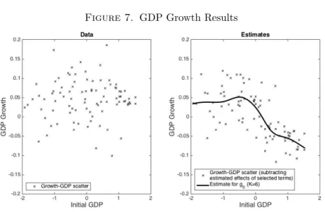
in this paper match those of [45]. Next, a simulation study demonstrates finite sample performance of the proposed procedure. Finally, an empirical example es-timating the relationship of initial GDP to GDP growth in a cross-section of 90 countries illustrates the use of Post-Nonparametric Double Selection.
2. Series estimation with a reduced dictionary
This section establishes notation, reviews series estimation, and describes series estimation on areduced dictionary. The exposition begins with basic assumptions on the observed data.
Assumption 1(Data). The observed data,Dn, is given byniid copies of random
variables(x, y, z)∈X×Y×Z indexed by16i6n, so that Dn= (yi, xi, zi)ni=1.
Here,yi are outcome variables,xi are explanatory variables of interest, and zi are
conditioning variables. In addition, Y⊆RandX⊆Rr for some integerr >0and
Zis a general measure space.
of the two concerns. In their paper, they prove that under the regularity right conditions, the two described model selection steps can be used to obtain asymptotically normal estimates ofα0 and
in turn to construct correctly sized confidence intervals.
10Alternative choices are possible and the analysis in the paper covers a general class of choices
Assumption 2 (Additive Separability). There is a random variable ε and func-tionsg0 andh0 such that the following additive separability11holds.
y=g0(x) +h0(z) +ε, E[ε|x, z] = 0.
Traditional series estimation of (g0, h0) is carried out by performing least squares
regression on series expansions in x and z. Define a dictionary of approximating functions by
(pK(x), qL(z)) where pK(x) = (p
1K(x), ..., pKK(x)) and qL(z) = (q1L(z), ..., qLL(z)) are each series of K and L functions such that their linear combinations can approxi-mate g0(x) and h0(z). Construct the matrices P = [pK(x1), ..., pK(xn)]0, Q = [qL(z
1), ..., qL(zn)]0,Y = (y1, ..., yn)0, and letβby,(K,L)= ([P Q]0[P Q])−1[P Q]0Y be
the least squares estimate from Y on [P Q]. Let [βby,(K,L)]g be the components of
b
βy,(K,L)corresponding to pK. Thenbg(x) is defined by b
g(x) =pK(x)0[βby,(K,L)]g.
WhenL > n, quality statistical estimation is only feasible provided dimension reduction or regularization is performed. A dictionary reduction selects new ap-proximating terms,
(pK(x), qL(z)) reduction−→ (˜p(x),q˜(z)),
comprised of a subset of the series terms in (pK(x), qL(x)). In this paper, be-cause the primary objects of interest center around g0(x), it will be the
conven-tion to always take ˜p(x) = pK(x). The post-model-selection estimate of g0(x)
is then defined analogously to the traditional series estimate. Let βby,( ˜p,q˜) =
([ ˜P Q˜]0[ ˜P Q˜])−1[ ˜P Q˜]0Y where ˜P = [˜p(x
1), ...,p˜(xn)]0 =P, ˜Q= [˜q(z1), ...,q˜(zn)]0 and as before, let [βby,( ˜p,q˜)]gbe the components ofβby,( ˜p,˜q)corresponding to ˜p. Then
b
g is defined by
b
g(x) = ˜p(x)0[βby,( ˜p,q˜)]g.
Finally, consider a functional12 a(g) ∈ R and as before, set θ0 = a(g0). One
sensible estimate forθ0is given by
b
θ=a(bg).
In order to use θb for inference on θ0, an approximate expression for the
vari-ance var(θb) is necessary. As is standard, the expression for the variance will
be approximated using the delta method. Let Ab =
∂a(pK(x)0b)
∂b ([βby,( ˜p,q˜)]g). Let
M= Idn−Q˜( ˜Q0Q˜)−1Q˜0 be the projection matrix onto the space orthogonal to the
11This assumption simply rewrites the equation stated in the introduction in terms of aresidual
ε. To ensure uniqueness ofg0, a further normalization is required. A common normalization in
the series context isg0(0) = 0, which is sufficient for most common assumptions onh0.
span of ˜Q.13 Finally, let bE =Y −[ ˜P ,Q˜]βby,( ˜p,q˜). Estimate Vb using the following sandwich form: b V =AbΩb−1ΣbΩb−1Ab b Ω =n−1P˜0MP˜ b Σ =n−1P˜0Mdiag(bE)2MP .˜
The following sections describe a dictionary reduction technique, along with regu-larity conditions, which imply that
n1/2Vb−1/2(θ0−bθ)→dN(0,1).
The practical value of the results is that they formally justify approximate Gauss-ian inference for θ0. An immediate corollary of the Gaussian limit is that for any
significance level γ ∈ (0,1), with c1−γ/2 the (1−γ/2)-quantile of the standard
Guassian distribution, it holds that
P(θ0∈[bθ−c1−γ/2n1/2Vb−1/2,θb−c1−γ/2n1/2Vb−1/2])→γ.
3. Dictionary Reduction by Post-Nonparametric Double Selection The previous section described estimation using a generic dictionary reduction. This section discusses one class of possibilities for constructing such reductions.
It is important to note that the coverage probabilities of the above confidence sets depend critically on how the dictionary reduction is performed. In particular, naive one-step methods will fail to produce correct inference. Formal results expanding on this point can be found, for instance, in [46], [40]. Heuristically, the reason resulting confidence intervals have poor coverage properties is due to model selection mistakes.
To address this problem, this section proposes a procedure for selecting ˜q(z). The new procedure is a generalization of the methods in [15] who work in the context of the partially linear model E[y|x, z] =α0x+h0(z). The methods described below
rely heavily on Lasso-based model selection. Therefore, a brief description of Lasso is now provided. The following description of Lasso, which uses an overall penalty level as well as term-specific penalty loadings follows [8] who are motivated by allowing for heteroskedasticity.
For any random variable v with observations (v1, ..., vn), theLasso estimate v onqL(z) withpenalty parameter λandloadings l
j is defined as a solution
b
βv,L,Lasso∈arg min
n X i=1 (vi−qL(zi)0b)2+λ L X j=1 |ljbj|. The correspondingselected set Iv,Lis defined as
Iv,L={j:βbv,L,Lasso,j 6= 0}. Finally, the correspondingPost-Lasso estimator is defined by
b
βv,L,Post-Lasso∈arg min
b:bj=0 forj /∈Iv,L
n
X
i=1
(vi−qL(zi)0b)2.
Lasso is chosen over other model selection possibilities for several reasons. Fore-most, Lasso is a simple, computationally efficient estimation procedure which pro-duces sparse estimates because of its ability to set coefficients identically equal to zero. In particular, |Iv,L| will generally be much smaller than n if a suitable penalty level is chosen. The second reason is for the sake of continuity with the previous literature; Lasso was used in [15]. The third reason is for concreteness. There are indeed many alternative estimation or model selection procedures which select a sparse set of terms which in principle can replace the Lasso. It is possible to instead consider general model selection techniques in the course of developing the subsequent theory. However, framing the discussion using Lasso allows explicit calculation of bounds and explicit description of tuning parameters. This is also helpful in terms of practical implementation of the procedures proposed below.
The quality of Lasso estimation is controlled by λ and lj. As the number of different Lasso estimations increases (ie. with increasingly many different variables
v), the penalty parameter must be increased to ensure quality estimation uniformly over all differentv. The penalty parameter must also be increased with increasing
L. However, higher λ typically leads to more shrinkage bias in Lasso estimation. Therefore, givenlj,λis usually chosen to be large enough to ensure quality perfor-mance, and no larger. See [8] for details.
For the sake of completeness, the Post-Double Selection procedure of [15] is now reproduced for a partially linear model specified by E[y|x, z] =α0x+h0(z).
Algorithm 1. Post-Double Selection for the Partially Linear Model. (Reproduced from [15]).
1. First Stage Model Selection Step. Perform Lasso regressionxonqL(z) with penaltyλFS and loadings lFS,j. LetIFS be the set of selected terms.
2. Reduced Form Model Selection Step. Perform Lasso regression y on qL(z) with penaltyλRF and loadings lRF,j. LetIRF be the set of selected terms.
3. Post-Model Selection Estimation. Set IPD = IFS ∪IRF and let ˜q(z) =
[qjL(z)]j∈IPD. Estimateα0 withαb based on least squares regression
14ofy
on [x,q˜(z)].
Appendix A contains details about one possible method for choosing λFS, λRF
as well aslFS,j,lRF,j. Arguments in [15] show that the choices of tuning parame-ters given in Appendix A are sufficient to guarantee a centered Gaussian sampling distribution ofαbforα0.
The simplest generalization of Post-Double Selection is to expand the first stage selection step into K steps. More precisely, for k = 1, ..., K, perform Lasso re-gression of pkK(x) on qL(z), and set IFS,k as the selected terms. Then define
IFS =∪Kk=1IFS,k and continue to the reduced form and estimation steps.15 This approach has a few disadvantages. First, the selected variables can depend on the particular dictionarypK(x). Ideally, the first stage model selection should be approximately invariant to the choice ofpK(x).
14In [15] heteroskedasticity-consistent standard errors are used for inference.
15A previous draft of this paper took this approach. Deriving theoretical results for this
Instead, consider a general class of test functions ΦK ={ϕ}. Concrete classes for test functions are provided below. In the first stage in Post-Nonparametric Double Selection, a Lasso step ofϕ(x) onqL(z) is performed for eachϕ∈ΦK.
Algorithm 2. Post-Nonparametric Double Selection
1. First Stage Model Selection Step. For each ϕ ∈ ΦK, perform Lasso re-gressionϕ(x) onqL(z) with penaltyλ
ϕ and loadings lϕ,j. Let Iϕ,L be the selected terms. LetIΦK =∪ϕ∈ΦKIϕ,Lbe the union set of selected terms.
2. Reduced Form Model Selection Step. Perform Lasso regression y on qL(z) with penaltyλRF and loadings lRF,j. LetIRF be the set of selected terms.
3. Post-Model Selection Estimation. Set IΦK+RF =IΦK∪IRF. Estimateθ0
usingθbbased on the reduced dictionary
(˜p(x),q˜(z)) = (pK(x),[qjL(z)]j∈IΦK+RF).
The following are several concrete, feasible options for ΦK. The first option is named the Span option. This option is suggested for practical use and is the main option in the simulation study as well as in the empirical example that follow.
ΦK,Span={ϕ(x)∈LinSpan(pK(x)) : var(ϕ(x))61}.
The theory in the subsequent section is general enough to consider other options for ΦK which might possibly be preferred in different contexts. Three additional examples are as follows.
ΦK,Graded ={p11(x)} ∪ {p12(x), p22(x)}...∪ {p1K(x), ..., pKK(x)} ΦK,Multiple={p (1) 1K(x), ..., p (1) KK(x)} ∪...∪ {p (m) 1K(x), ..., p (m) KK(x)}} ΦK,Simple={p1K(x), ..., pKK(x)}.
Appendix A again contains full implementation details for the Span option. This includes one possible method for choosingλϕ,lϕ,j as well aslFS,j,lRF,j which yield favourable model selection properties. Discussion of the most important details is given in the text below. The analysis in the next section gives conditions under whichθbattains a centered Gaussian limiting distribution.
Choosing ΦK optimally is an important problem, which is similar to the prob-lem of dictionary selection.16 The Span option, Φ
K,Span is used in the simulation
study as well as in the empirical example, since it performed well in initial sim-ulations. Note that the definition of the set ΦK,Span depends on a population
quantity var(ϕ(x)) which may be unknown to the researcher. Note however, that the identities of the covariates selected in the Lasso-based procedure described in the appendix are invariant to rescaling of the left-hand side variable. The invariance
16The question of which option for Φ
K is optimal is likely application dependent. In order to
maintain focused, this question is not considered in detail in this paper but might be of interest for future work.
is a consequence of the method for choosing penalty loadings. Therefore, replac-ing the condition supx∈Xkϕ(x)k261 with var(ϕ(x))61 is possible. The option
ΦK,Simple is the direct extension of Post Double Selection as given in [15]. The
set ΦK,Multiple corresponds to using multiple dictionaries, indexed (1), ...,(m) in
the notation above. For example ΦK,Multiple could include the union of B-splines,
orthogonal polynomials, and trigonometric polynomials, all in the first stage selec-tion. The ΦK,Graded is appropriate when dictionaries are not nested with respect
toK. These include B-splines.
In order to set up a practical choice of penalty levels, the set proposed above, ΦK is considered as a union17: ΦK,Span= ΦK1∪ΦK2∪ΦK3 where ΦK1={x} ΦK2={p1K(x), ..., pKK(x)} ΦK3={ϕ(x)∈LinSpan(pK(x)) : var(ϕ(x))61}.
The reason then for decomposing ΦK,Spanin this way is allow the use of different
penalty levels on each of the three sets ΦK1,ΦK2,ΦK3. In particular,λΦK1 is the
penalty for a single heteroskedastic Lasso as described in [8]. λΦK2 is a penalty
which adjusts for the presence ofK different Lasso regressions withK→ ∞. The main proposed estimator sets λΦK3 = λΦK2. This is less conservative than the
penalty level would be following [10] for a continuum of Lasso estimations.18 As a result, any corresponding Lasso performance bounds do not hold uniformly over ΦK3. Rather the implied bounds hold only uniformly over any pre-specified K
element subsets of ΦK3. The high-level model selection assumption below (see
As-sumption 10) indicates that these bounds are sufficient for the present purpose. In the simulation study, a more conservative (higher) choice forλΦK3 is also
consid-ered. In terms of inferential quality, there is no noticeable difference between the two choices of penalties in the data generating processes considered in the simu-lation study. As discussed above, penalty levels accounting for a set of different Lassos estimated simultaneously must be higher to ensure quality estimation. This leads to higher shrinkage bias. The above decomposition therefore addresses both concerns about quality estimation and shrinkage bias by allowing smaller penalty levels to be used on subsets of ΦK,Span. Because the decomposition is into a fixed,
finite number of terms (ie. into 3 terms), such an estimation strategy presents no additional theoretical difficulties.
Another practical difficulty with this approach is computational. It is infeasible to estimate a Lasso regression for everyϕindexed by a continuum. Therefore, some approximation must be made. The reference [10] gives suggestions for estimating a continuum of Lasso regressions using a grid. This may be computationally expen-sive ifK is even moderately large. An alternative heuristic approach is motivated by the observation thatqjL is selected intoIΦK only when there is ϕ∈ΦK such
thatj∈Iϕ,L. In the context of estimatingθ0, only the identity of selected terms is 17Some dictionariespK(x) may not contain a termpkK(x) =x. In this case,ϕ(x) =xcan
be appended to ΦK. In addition, after rescaling, ΦK1⊆ΦK2⊆ΦK3is possible, and so the sets
have nonempty intersection. This causes no additional problems.
18Note, the normalization thatkϕ(x)k2
61 ensures that ΦK3is indexed by a compact set and
important (not their coefficients). For the implementation in this paper, a strategy for approximatingIΦK is adopted where for eachj 6L, a Lasso regression is run
using exactly one test function, ˇϕj∈ΦK. The choice of ˇϕj is made based on being likely to select qjL relative to otherϕ∈ ΦK. Specifically, for each j, ˇϕj is set to the linear combination of p1K, ..., pKK with highest marginal correlation to qjL. Then the approximation to the first stage model selection step proceeds by using
ˇ
IΦK = S
j6LIϕˇj(x)in place ofIΦK. This is also detailed in the appendix.
The formal theory in the subsequent sections proceeds by working with a notion of density of ΦKwithin a broader space of approximating functions forg(x). Aside from added generality, working in this manner is helpful since it adds structure to the proofs and it isolates exactly how the density of ΦK interacts with the final estimation quality forθ0.
4. Formal Theory
In this section, additional formal conditions are given which guarantee con-vergence and asymptotic normality of the Post-Nonparametric Double Selection. There are undoubtedly many aspects of the estimation strategy that can be ana-lyzed. These include important choices of tuning parameters andK.
The following definition helps characterize smoothness properties of target func-tion g0 and approximating functions pK. Let g be a function on X. Define the
Sobolev norm|g|d = supx∈Xmax|c|6d|∂|c|g/∂xc|where the inner maximum ranges over multi-indecesc.
Assumption 3 (Regularity for pK). For each K, there is a nonsingular matrix
BK such that the smallest eigenvalue of the matrix ΩBKpK = E
BKpK(x)(BKpK(x))0
is bounded uniformly away from zero in K. In addition, there is a sequence of constants ζ0(K)satisfyingsupx∈XkBKpK(x)k26ζ0(K)andn−1ζ0(K)2K→0 as
n→ ∞.
Assumption 4 (Approximation ofg0). There is an integerd>0, a real number
αg0 > 0, and a sequence of vectors βg0,K which depend on K such that |g0− pK0βg0,K|d=O(K
−αg0)asK→ ∞.
Assumptions 3 and 4 would be identical to Assumptions 2 and 3 from [45] if there was no conditioning variable z present. These assumptions require that the dictionarypKhas certain regularity and can approximateg
0at a pre-specified rate.
The quantityζ0(K) is dictionary specific, and can be explicitly calculated in certain
cases. For instance, [45] gives that ζ0 = O(K1/2) is possible for B-splines. Note
that values of αg0 can be derived for particular d, p
K, and classes of functions containingg0. [45] also gives explicit calculation ofαg0 for the leading cases when pK(x) are power series and regression splines.
The next assumption quantifies the density of ΦK within LinSpan(pK). In order to do so, define the following. Let
ρ(g,ΦK) = inf
kg>1, η=(η1,...,ηkg)∈Rkg,ϕ1,...,ϕkg∈ΦK
LαZsup
Assumption 5 (Density of ΦK). Each ϕ∈ΦK satisfiesvar(ϕ(x))61. There is
a constant αρ>0 such that sup
{g∈LinSpan(pK): var(g(x))61}
ρ(g,ΦK) =O(Kαρ).
There is nothing special about the constant 1 in var(ϕ(x))61. It is mainly a tool for helping describe the density of ΦK. In addition, as mentioned above, the set selected by Lasso as described in the appendix is invariant to rescaling of the left-hand side variable. As a result, imposing restrictions on var(ϕ(x)) is without loss of generality.
The density assumption is satisfied with αρ = 0 if the ΦK = ΦK,Span is used
since in that case, ρZ(g,ΦK) is bounded uniformly in g. On the other hand, the density assumption may only be satisfied with αρ = 1/2 or higher for the basic ΦKSimple={p1K(x), ..., pKK(x)} option.
The next assumptions concern sparse approximation properties of qL(z). Two definitions are necessary before stating the assumption. First, a vectorX is called
s-sparse if |{j : Xj 6= 0}| 6 s. Next, let πqL denote the linear projection
oper-ator. More precisely, for a square integrable random variable v, πqLv is defined
byπqLv(z) =qL(z)0βv,L forβv,L such that E[(v−qL(z)0βv,L)2] is minimized. For functionsϕofxsuch thatϕ(x) is square integrable, writeβϕ,L=βϕ(x),L.
Assumption 6(Sparsity). There is a sequences0>1and a constantαZ >0such
that the following hold.
1. There is a sequence of vectors βh0,L,s0 that are s0-sparse with support S0 such that supz∈Z|h0(z)−qL(z)0βh0,L,s0|=O(L
−αZ).
2. For allϕ∈ΦKthere are vectorsβϕ,L,s0 that ares0-sparse, all with common supportS0, such that
sup ϕ∈ΦK sup z∈Z| πqLϕ(z)−qL(z)0βϕ,L,s0|=O(L −αZ).
Assuming a uniform bound for the sparse approximation error for h0 is
poten-tially stronger than necessary. At the moment of the writing of the manuscript, the author sees no theoretical obstacle in terms of working under the weaker assump-tionn−1Pn
i=1|h0(zi)−qL(zi)0βh0,L,s0|
2=O
p(L−αZ). In addition, theL−αZ rate is imposed in order to maintain a parallel exposition relative to theO(K−αg0) term.
Other rates, for instancen−αZ, can also replace L−αZ, and this is done in [15], [8] and other references.19 The same comment holds for the sparse approximation
conditions forϕ∈ΦK.
Several references in the prior econometrics literature work with sparse approx-imation of the conditional expectation rather than the linear projection. In this context, working with the conditional expectation places a higher burden on the approximating dictionaryqL. In particular, If the conditional expectation of ϕ(x) givenzcan be approximated usings0 terms fromqL, then the conditional
expecta-tion ofϕ(x)2may potentially requireO(s20) terms to approximate once interactions are taken into account. This potentially requires the dictionary qL to contain a prohibitively large amount of interaction terms. For this reason, the conditions in this paper are cast in terms of linear projections.20
19usingn−αZ is only more general ifLgrows faster than every polynomial ofn.
20The author sees no theoretical obstructions in terms of applying the same arguments for
The next assumption imposes limitations on the dependence betweenx andz. For example, in the case that ϕ(x) = x is an element of pK(x), this assumption states that the residual variation after a linear regression ofxonzis non-vanishing. More generally, the assumption requires that population residual variation after projectingpkK(x) away fromz is non-vanishing uniformlyK, L. One consequence of Assumption 7 is that constants cannot be freely added to bothg0(x) andh0(z).
This therefore requires the user to enforce a normalization condition likeg0(0) = 0
or E[g0(x)] = 0.The simulation study and empirical illustration below both enforce
g0(0) = 0.
Assumption 7(Identifiability). For eachK and for BK as in Assumption 3, the
matrixE[BK(pK(x)−πqLpK(z))(BK(pK(x)−πqLpK(z)))0]has eigenvalues bounded uniformly away from zero inK, L. In addition,supz∈ZkBKπqLpK(x)k26ζ0(K).
The next condition restricts the sample Gram matrix of the second dictionary. A standard condition for nonparametric estimation is that for a dictionaryP, the Gram matrixn−1P0Peventually has eigenvalues bounded away from zero uniformly innwith high probability. IfK+L > n, then the matrixn−1[P Q]0[P Q] will be rank deficient. However, in the high-dimensional setting, to assure good performance of Lasso, it is sufficient to only control certain moduli of continuity of the empirical Gram matrix. There are multiple formalizations of moduli of continuity that are useful in different settings, see [17], [59] for explicit examples. This paper focuses on a simple condition that seems appropriate for econometric applications. In par-ticular, the assumption that only small submatrices ofn−1Q0Qhave well-behaved
eigenvalues will be sufficient for the results that follow. In the sparse setting, it is convenient to define the following sparse eigenvalues of a positive semi-definite matrixM:21 κmin(m)(M) := min 16kδk06m δ0M δ kδk2 2 , κmax(m)(M) := max 16kδk06m δ0M δ kδk2 2 .
In this paper, favorable behavior of sparse eigenvalues is taken as a high level condition and the following is imposed.
Assumption 8 (Sparse Eigenvalues). There is a sequence sκ = sκ(n) such
that sκ → ∞ and such that the sparse eigenvalues obey κmin(sκ)(n−1Q0Q)−1 =
O(1)andκmax(sκ)(n−1Q0Q) =O(1) with probability1−o(1).
The assumption requires only that sufficiently small submatrices of the largep×p
empirical Gram matrixn−1Q0Qare well-behaved. This condition seems reasonable
and will be sufficient for the results that follow. Informally it states that no small subset of covariates inqL suffer a multicollinearity problem. They could be shown to hold under more primitive conditions by adapting arguments found in [9] which build upon results in [57] and [49]; see also [48].
argument is that expressionPn
i=1qL(zi)(πqL(zi)−qL(zi)βϕ,L) stays suitably small. Note this expression is a sum of mean zero independent random variables in the present context.
21In the sparse eigenvalue definition,k · k0refers to the number of nonzero components of a
Assumption 9 (High-Level Model Selection Performance). There are constants αIΦ andαΦ and bounds
1. |IΦK|6K αIΦO(s0) 2. supϕ∈ΦKPn i=1(qL(zi)0(βϕ,L,s0−βbϕ,L,Post-Lasso)) 2 =O(KαΦs 0log(L)) 3. |IRF|=O(s0) 4. Pn i=1(q L(z
i)0(βy,L,s0−βby,L,Post-Lasso))
2 =O(s
0log(L))
which hold with probability1−o(1).
The standard Lasso and Post-Lasso estimation rates when there is only one outcome considered ares0log(L) for the sum of the squared prediction errors, and
O(s0) for the number of selected covariates. Therefore, KαΦ is a uniform measure
of the loss of estimation quality stemming from the fact that Lasso estimation is performed on all ϕ ∈ΦK rather than just on a single outcome. Similarly, KαIΦ
measures the number of uniquej selected in all first stage Lasso estimations. The choice to present high-level assumptions is for generality - so that other model selection techniques can also be applied. However, verification of the high level bounds are available under additional regularity for Lasso estimation.
One reference on performance bounds for a continuum of Lasso estimation steps is [10]. In that paper, the authors provide formal conditions (specifically Assump-tion 6.1) and prove that Statement 2 of AssumpAssump-tion 9 holds. The bounds in that reference correspond to takingαΦ= 1/2. An important note is that the conditions
in [10] are slightly more stringent since the authors assume thatβϕ,L,s0 andβy,L,s0
can be taken to approximate the conditional expectation of ϕ(x) and y given z
rather than just the linear projection. When|ΦK|finite, but grows only polynomi-ally withnandL > n,αΦ= 0 is possible under further regularity conditions.
The main theoretical difficulty in verifying Assumption 9 using primitive condi-tions is in showing that the size of the setIΦKstays suitably small. [10] prove certain
performance bounds for a continuum of Lasso estimates under the assumption that dim ΦK is fixed and state that their argument would hold for certain sequences dim ΦK → ∞. [10] also proves that the size of the supports of the Lasso estimates, |Iϕ,L|stay bounded uniformly by a constant multiple of s0which does not depend
on nor ϕ. They do not, however, prove that the size of the union | ∪ϕ∈ΦKIϕ,L|
remains similarly bounded. Therefore, their results do not imply a the existence of a finite value ofαIΦ. The later bound is required for the analysis of the above
proposed estimator. For a finite approximation to ΦK,Span (like ΦK,Simple), there
is no difficulty calculating bounds on the total number of distinct selected terms. This is because under regularity conditions standard in the literature, each Iϕ,L satisfies |Iϕ,L| 6 O(s0) where the implied constants in the O(s0) terms can be
bounded uniformly overϕ∈ΦK. In particular, when ΦK is finite, it is possible to takeKαIΦ =|ΦK|. This paper does not derive a bound for|IΦ
K,Span|as this would
likely lie outside the scope of this project. A valid alternative for which verifiable bounds on the union of selected covariates is possible is to report estimates using
b
ΦK =
(
ΦK,Simple on the event that |IΦK,Span|> t(n)
ΦK,Span otherwise.
When{g∈LinSpan(pK) : var(g(x))61} coincides with ΦK, so that ΦK is as dense as possible, then Assumption 9 can be weakened in the following.
Assumption 10(Alternative High-Level Model Selection Performance ). Suppose that {g ∈LinSpan(pK) :var(g(x))
61} ⊆ΦK. LetΦK0 ⊂ΦK be any nonrandom
fixed finite subset of at most K elements. There are constants αIΦ and αΦ and bounds 1. |IΦK|6K αIΦO(s 0) 2. supϕ∈Φ K0 Pn i=1(q L(z i)0(βϕ,L,s0−βbϕ,L,Post-Lasso)) 2 =O(KαΦs 0log(L)) 3. |IRF|=O(s0) 4. Pn i=1(q L(z
i)0(βy,L,s0−βby,L,Post-Lasso))
2 =O(s
0log(L))
which hold with probability1−o(1).
Assumption 10 is weaker than Assumption 9. However, Assumption 9 can be more easily verified with primitive conditions by using finite sets ΦK.
Statements 2-4 can be attained under standard conditions withαΦ= 0 provided
a penalty adjusting forK different Lasso estimations is used. On the other hand, using a conservative penalty as in [10] for the continuum of Lasso estimations like in ΦK,Span would result in αΦ= 1/2. There is currently no proof that Statement
1 with αIΦ = 0 and Statement 2 with αΦ = 0 can hold simultaneously under
conditions standard in the econometrics literature.
It is interesting to note that the requirements to satisfy Assumption 10 are essen-tially pointwise bounds on the predictive performance of a set of Lasso estimations along with a uniform bound on the identity of selected covariates. By contrast, [10] prove uniform bounds on Lasso estimations along with pointwise bounds on the identity of selected covariates. In practice, verification of the Condition 1 in As-sumption 10 could be potentially very useful. This would allow the researcher to use a penalty level which is smaller by a factor ofK1/2, and would ultimately allow
more robustness without increasing variability of the final estimator.
For the choice of penalty parameters given in Appendix A for the Span option, Conditions 2-4 of Assumption 10 can be verified under further regularity condi-tions like those given in [10] or [8] to yield αΦ = 0. Furthermore, Condition 1
of Assumption 10 can be verified if an option like ΦbK mentioned on the previous page is used. Most importantly, Assumption 10 serves a plausible high-level model selection condition which is sufficient for proving the results that follow.
The next assumption describes moment conditions needed by applying certain laws of large numbers, for instance for the quantitiesn−1Pn
i=1ε 2
iqjL(zi)2.
Assumption 11 (Moment Conditions). The following moment conditions hold.
1. E[qjL(z)2[BK(pK(x)−πqLpK(z))]2k] is bounded away from zero uniformly inK, L
2. E[|qjL(z)|3]is bounded uniformly in L
3. E[qjL(z)2ε2] is bounded away from zero uniformly inL 4. E[|qjL(z)|3|ε|3]is bounded uniformly in L.
The first statement of the assumption may also be seen as a stricter identifi-ability condition condition on the residual variation pK(x)−π
qLpK(z). It rules
out situations where for instance x6= 0 ⇔qjL(z) = 0. Note that E[[BK(pK(x)−
is needed about the corresponding third moment E[[BK(pK(x)−πqLpK(z))]3k] = 1
since instead a reference to the boundζ0(K) is used.
The final assumption before the statement of Theorem 1 are rate conditions.
Assumption 12 (Rate Conditions). The following rate conditions hold.
1. s0KαIΦ =o(sκ) 2. log(KL) =o(ζ0(K)−1n1/3) 3. L−αZn1/2K−1/2ζ 0(K) =O(1) 4. L−2αZK2αρ(K1/2n1/2ζ 0(K)−1+n1/2+Klog(L)1/2ζ0(K)−2) =O(1) 5. n−1/2K1/2s0log(L)ζ0(K)−1(K2αρ+αΦ+Kαρ+αΦ/2+αIΦ/2) =O(1) 6. n−1/2s10/2log(L)(K2αρ+αΦs1/2 0 +K αIΦ/2) =O(1).
The first statement ensures that the sparse eigenvalues remain well-behaved in the with high probability over sets whose size is larger that the selected covari-ates. The second statement is used in conjunction with the above moment con-ditions to allow the use of moderate deviation bounds following [37]. The third and fourth conditions are assumption on the sparse approximation error forqL(z). The final two assumptions restrict the size of s0 and K and quantities
depend-ing on αρ, αΦ, and αIΦ relative to n. These assumptions can be unraveled for
certain choices of dictionaries. For example, as was noted above and by [45], for B-splines,ζ0(K) can be taken to beO(K1/2).Using the simple option givesαρ = 1,
αΦ= 0 and αIΦ = 1. Then the conditions can be reduced to L
−αZn1/2 =O(1),
L−2αZK2n1/2=O(1),n−1/2K2s
0log(L) =O(1).
The first result is a preliminary result which gives bounds on convergence rates for the estimatorbg. They are used in the course of the proof of Theorem 1 below, the main inferential result of this paper. The proposition is a direct analogue of the rates given in Theorem 1 of [45] which considers estimation of a conditional expectationg0
without model selection over a conditioning set. The rates obtained in Proposition 1 match the rates in [45]. To state it, let F0 be the distribution function of the
random variablex. In addition, letζd(K) = max|c|6dsupx∈Xk∂|c|BKpK(x)/∂xck2.
Theorem 1. Under Assumptions 1-8, 9 or 10, and 11-12, the Post-Nonparametric Double Selection estimategbfor the function g0 satisfies the following bounds.
Z
(bg(x)−g0(x))2dF0(x) =Op(n−1K+K−2αg0).
|bg−g0|d =Op(n−1/2ζd(K)K1/2+K−αg0).
The next formal results concern inference for θ0 = a(g0). Recall that θ0, is
estimated bybθ=a(bg) and inference is conducted via the estimatorVb as described
in earlier sections.
Assumption 13(Moments for Asymptotic Normality). E[ε4+δ|x, z]is bounded for
someδ >0. var(ε|x, z) is bounded away from zero.
Note that the conditions in [45] require only that E[ε4|x, z] is bounded. The
strengthened condition is needed for consistent variance estimation, in order to construct a bound on the quantity maxi6nε2i.
The following assumptions on the functionalaare imposed. They are regularity assumptions that imply thataattains a certain degree of smoothness. For example, they imply thatais Fr´echet differentiable.
Assumption 14 (Differentiability for a). The real valued functional a(g) ∈ R is either linear or the following conditions hold. n−1ζd(K)4K2 → 0. There is a
linear functionD(g; ˇg)that is linear in g and such that for some constantsC, ν >
0 and all ˇg,gˇˇ with |g −g0|d < ν, |ˇg −g0|d < ν, |gˇˇ−g0|d < ν, it holds that |a(g)−a(ˇg)−D(g−ˇg; ˇg)|6C(|g−gˇ|d)2 and|D(g; ˇg)−D(g; ˇgˇ)|6C|g|d|ˇg−ˇˇg|d.
The functionDis related to the functional derivative ofa. The following assump-tion imposes further regularity on the continuity of the derivative. For shorthand, letD(g) =D(g;g0).
The next rate conditions is used to ensure that estimates are undersmoothed. The rate condition ensures that the estimation bias, which is heuristically captured byK−αg0, converges to zero faster than the estimation standard error.
Assumption 15 (Undersmoothing Rate Condition). n1/2K−αg0 =o(1).
The next rate condition is used in order to bound quantities appearing in the proof of Theorem 2. As was demonstrated in the case of Assumption 12, the rate conditions can be unraveled for certain choices ofK,pK, and ΦK.
Assumption 16 (Rate Conditions for Asymptotic Normality).
1. L−2αZK2αρ(ζ 0(K)K+ζ0(K)4K1−2αρ+Klog(L) +n1/2) =o(1) 2. n−1s 0ζ0(K) log(L)(K1+2αρ+αΦ+K1+αρ+αΦ/2+αIΦ/2) =o(1) 3. n−1s20log(L)2(K4αρ+2αΦ+K2αρ+αΦ+αIΦ) =o(1) 4. s0KαIΦ n−1/2ζ0(K)K1/2+K−αg0=o(1) 5. n2/(4+δ)ζ 0(K)n−1/2K1/2=o(1).
The final two conditions divide the cases considered into two classes. The first class (covered by Assumption 17) are functionals which fail to be mean-square dif-ferentiable and therefore cannot be estimated at the parametric n1/2 rate. The second class (covered by Assumption 18) does attain the n1/2 rate. One example with the functional of interest is evaluation ofgat a pointx0: a(g) =g(x0). In this
case,afails to be estimated that the parametricn1/2rate in general circumstances.
A second example is the weighted average derivative a(g) = R
w(x)∂g(x)/∂x for a weight function w which satisfies regularity conditions. The Assumption 18 holds if w is differentiable, vanishes outside a compact set, and the density ofx
is bounded away from zero whereverwis positive. In this case,a(g) = E[ψ(x)g(x)] for ψ(x) = −φ(x)−1∂w(x)/∂x by a change of variables provided that x is con-tinuously distributed with non vanishing density φ. These are one possible set of sufficient conditions under which the weighted average derivative does achieve √
n-consistency.
Assumption 17 (Regularity for a in Absence of Mean-Square Differentiability). There is a constant C >¯ 0 such that|D(g)|6C¯|g|d. There is β¯ dependent on K
such that forg¯(x) =p(x)K0β¯, it holds thatE[¯g(x)2]→0andD(¯g)
>C >¯ 0. Assumption 18 (Conditions for n1/2-Consistency). There is ψ(x) such that
E[ψ(x)2] finite and nonzero and such that D(g) = E[ψ(x)g(x)] and D(pkK) = E[ψ(x)pkK(x)] for every k. There is β˘ such that E[(ψ(x)−p(x)K
0˘
β)2] → 0.
Fi-nally, the matrixV¯ = E[ψ(x)2var(y|x, z)] is finite and nonzero.
Theorem 2 now establishes the validity of standard inference procedure after model selection as well as validity of the plug in variance estimator.
Theorem 2. Under Assumptions 1-8, 9 or 10, 11-17, the Post-Nonparametric Double Selection estimate for the functionθ0 satisfies
b θ=θ0+Op(n−1/2ζd(K)). In addition, n1/2V−1/2(θb−θ) d →N(0,1) and n1/2Vb−1/2(θb−θ) d →N(0,1). Under Assumptions 1-8, 9 or 10, 11-16, and 18,
n1/2(θb−θ)
d
→N(0,V¯) and V −V¯ →p 0.
5. Simulation study
The results stated in the previous section suggest that Post-Nonparametric Dou-ble Selection series estimation should exhibit good inferential properties for addi-tively separable conditional expectation models when the sample sizenis large. The following simulation study is conducted in order to illustrate the implementation and study the performance of the outlined procedure.
The simulation study is divided into two parts. The first part compares several alternative estimators to Post-Nonparametric Double Selection. The second part compares several Post-Nonparametric Double Selection estimates using different choices for ΦK. This part demonstrates finite sample benefits from using the Span option relative to the direct generalization of Post-Double Selection estimation (ie. using the Simple option).
The following process generates the data in each simulation.
y=g0(x) +h0(z) +ε g0(x) = 10 sin(0.1x)−0.5 sin(4πx4−x 2 ) h0(z) =z0βh0,L, βh0,L,j=−0.5·(−0.65) j−11 j6s0 zj∼N(0,1), corr(zj1, zj2) = 0.25 |j1−j2| ε∼N(0,1) x= 0.15v+ 0.0375−3.75(stair(z0γ0+v) + 0.375)FN(0,1)(10zs0)... + 3.75(stair(0.5(z0γ0+v)|z0γ0+v|0.25)(1−FN(0,1)(10zs0)) γ0,L,j =−1.5(−0.75)j−11j6s0 v∼N(0,1) stair(·) = 0.25tanh(12(·)/2.5)−12b(·)/2.5c −6 2 tanh(6) + 0.5 +b(· )/2.5c .
The study performs simulations forn∈ {100,150, ...,500}. Two settings for the parameterL are considered: L=n/2 andL= 2n. Finally, the sparsity level is set to s0 = 6. Within each data generating process, 1000 simulation replications are
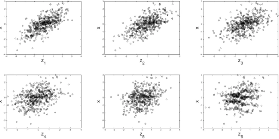
The data generating process is quite complicated. It is designed in order to create correlations between the covariateszand various transformations ofx. This allows the data generating process to highlight many different statistical problems which can arise using Nonparametric-Post Double Selection and alternative estimation techniques all in one simulation study. Despite the complicated formulas for the joint distribution ofxandz, their realizations appear natural. Scatter plots of one sample ofn= 500 showing the respective bivariate distributions betweenz1, ..., z6
andxare provided in Figure 6. Figure 5 provides a picture of the graph ofg0.
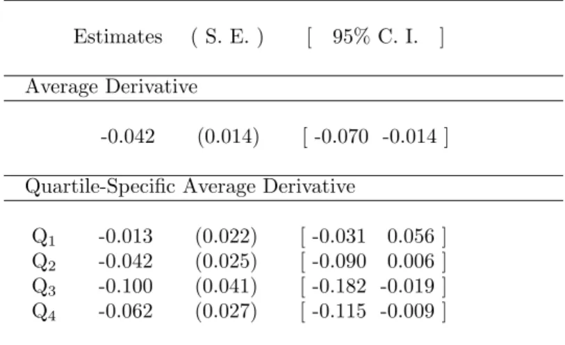
The simulations evaluate estimation ofg0 and ofθ0 defined by
θ0= E[g00(x)].
In order to avoid further complications, for each replication, the expectation and thus trueθ0 are calculated against the empirical distribution ofxwithin that
sim-ulation replication.22
The first part of the simulation study considers the performances of five estima-tors23for g
0 and θ0. Each estimator is a reduced series estimator based on initial
dictionaries consisting of a cubic spline expansion pK(x) for g0(x) and a linear
expansionqL(z) =zforh0(z).
1. Oracle. Estimator 1 is infeasible and sets ˜q(z) = (z1, .., zs0). This
estima-tor serves as a benchmark for comparison to estimates in which the correct support is known.
2. Span Post-Nonparametric Double. Estimator 2 selects ˜q(z) using Post-Nonparametric Double Selection with Φk given by the Span option, as described in this paper.
3. Naive. Estimator 3 selects ˜q(z) in one model selection step by performing Lasso ofy onqL(z).
4. OLS.Estimator 4 uses ˜q(z) = z. In other words, this estimator does not reduce the dictionary. This estimation strategy is only calculated provided
L < n.
5. Targeted Undersmoothing. Estimator 5 implements an alternative in-ferential procedure for dense functionals of high-dimensional parameters; TU(1). This procedure was proposed in [30] and is described further be-low.
22Another possibility is to calculate against the population expectation ofx. Under the
as-sumption that the researcher knows the population distribution ofx, this causes no further com-plication. If the distribution ofx is unknown and estimated, this must however be taken into account.
23There are likely other sensible estimators beyond the 5 considered in the simulation section.
As pointed out by an anonymous reviewer, such estimators may include propensity score matching on a continuous variable. Though such an approach may work well, the context here is not exactly the same as usually seen in propensity score matching. In particular, the assumptions here do not require unconfoundedness conditions. In addition, propensity score techniques are most commonly applied to discrete treatement variables. There is some work on propensity score matching with a continuous treatment; for example, see [35], who require the estimation of the conditional density of treatment. In the high-dimensional setting, estimating the conditional density ofx given z
Detailed implementation descriptions are provided in Appendix A. For each of the above estimators, the choice of pK(x) is made using a data-dependent rule. First, an initial dictionary reduction qinitial(z) is selected. For Oracle,
qinitial(z) = (z
1, .., zs0). For the Span Post-Nonparametric Double and Naive
es-timators,qinitial(z) is based on Lasso ofy onqL(z) as implemented in Appendix A. For OLS,qinitial(z) =z. Next, BIC is used to choose a B-spline expansionpK(x).
Comparison of estimators 1-4 is standard in the post-model selection economet-rics literature. The oracle estimator should be seen as a benchmark which is known to provide good estimates if the true set, S0, was known. The Naive estimator is
expected to perform poorly since it is not a uniformly valid estimator and suscep-tible to size-distortions arising from model selection mistakes. OLS is expected to perform poorly due to potential problems related to overfitting.
Estimator 5 is a procedure called Targeted Undersmoothing which looks to cor-rect distortions in inference from model selection mistakes. Targeted Undersmooth-ing appends covariates which significantly affect the value of the functionalθb=a(bg)
to an initially selected model (see [30]). It is appropriate for functionals of high-dimensional models which depend on a growing number of parameters (dense func-tionals) and is therefore a potentially sensible procedure for inference for θ0. This
estimator is detailed further in Appendix A.
The simulation results report several quantities which measure the performance of each estimator. The results report standard deviation of the estimatesθb, bias
of the estimates for θ0, confidence interval length for estimates for θ0, rejection
frequencies under the null for θ0 at the 5% level, mean number of series termsK
used, mean number of series terms selected from the original L, and integrated squared error forg0. The simulation results are reported in Figure 1 forL =n/2
and Figure 2 forL= 2n. The figures display the above mentioned simulation results for eachn= 100, ...,500 withnchanging over the horizontal axis.24 Note also that
across some of the estimators, some of the reported quantities will be identical. For example, the point estimates for TU are identical to the Naive point estimates. The selectedK is identical for the Naive estimates as well as the Post-Nonparametric Double Selection estimates.
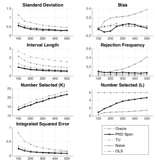
In all of the simulations, the Post-Nonparametric Double Selection estimates behave similarly to the Oracle estimates. The OLS estimates have wide confidence intervals relative to the Post-Nonparametric Double Selection estimation, but have similar coverage properties. The final estimator, Targeted Undersmoothing (TU), is conservative in terms of coverage, with substantially larger intervals in every case. On the other hand, the Naive estimator has poor coverage properties. For the Naive estimator, after failing to control for the correct covariates, the increase inK
leads to an increasing bias. This highlights the fact that simply producing under-smoothed estimates ofg0 by increasingK may not be adequate for reducing bias
and making quality statistical inference possible in the high-dimensional setting.
24Note that sinces
0, the magnitude of coefficientsβh0,L and the joint distribution between
relevant covariates are all fixed in the simulations asn→ ∞. Therefore, for sufficiently largen, all relevant covariates would be identified with high probability, and all of the post-model selection estimators would perform similarly. This simulation study therefore is identifying differences in finite sample performance.
Figure 1. Simulation Results
This figure presents simulation results for the estimation ofg0andθ0in the cases
n= 100,150, ...,500 withs0= 6 andL=n/2 according to the data generating process described
in the text. Estimates are presented for the five estimators, Oracle, Post-Nonparametric Double (PND Span), Naive, OLS and Targeted Undersmoothing (TU) as described in the text. The first plot shows standard deviation of the respective estimates forθ0. The second plot shows bias of
the estimates forθ0. The third plot shows confidence interval length for estimates forθ0. The
fourth plot shows rejection frequencies under the null forθ0 for a 5% level test. The fifth plot
shows the mean number of series termsKused. The sixth plot shows the mean number of series terms fromLselected. The seventh plot shows root mean integrated squared error forg0.
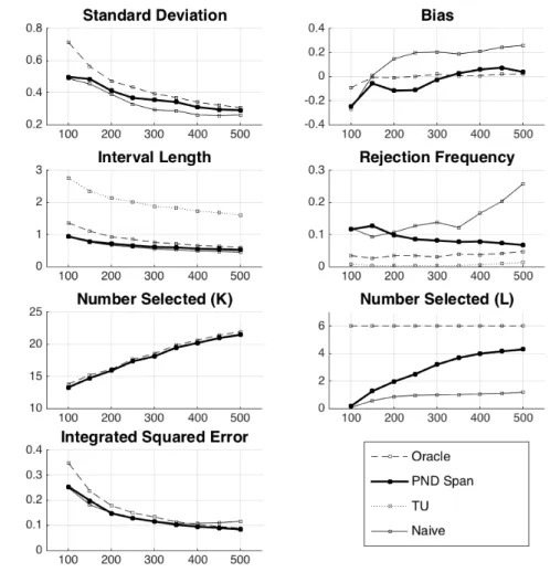
Figure 2. Simulation Results
This figure presents simulation results for the estimation ofg0andθ0in the cases
n= 100,150, ...,500 withs0= 6 andL= 2naccording to the data generating process described
in the text. Estimates are presented for the four estimators, Oracle, Post-Nonparametric Double (PND Span), Naive, and Targeted Undersmoothing (TU) as described in the text. The first plot shows standard deviation of the respective estimates forθ0. The second plot shows bias of the
estimates forθ0. The third plot shows confidence interval length for estimates forθ0. The fourth
plot shows rejection frequencies under the null forθ0for a 5% level test. The fifth plot shows the
mean number of series termsKused. The sixth plot shows the mean number of series terms fromLselected. The seventh plot shows root mean integrated squared error forg0. In each plot,
the horizontal axis denotes sample sizen. Figures are based on 1000 simulation replications. nis always indexed by the horizontal axis.
The second part of the simulation study compares four Post-Nonparametric Dou-ble Selection estimators which use different specifications for ΦK.
1. Span Post-Nonparametric Double. Estimator 1 is identical to the Span Post-Nonparametric Double estimator in the first part of the simulation. 2. Conservative Span Post-Nonparametric Double. Estimator 2 uses
pK and Φ
K as in the Span option, but in the decomposition ΦK,Span =
ΦK1∪ΦK2∪ΦK3, the penalty applied to ΦK3is more conservative,
explic-itly aimed at achieve Lasso performance bounds which hold uniformly over all of ΦK.
3. Simple Post-Nonparametric Double. Estimator 3 uses pK as in the Span, but uses ΦK = ΦK,Simple.
4. Alternative Spline Basis Simple Post-Nonparametric Double. Es-timator 4 uses a different basis for selection. A QR decomposition is applied to P in order to obtain orthonormal columns. Next, ΦK = ΦK,Simple is
used on the new orthogonalized data. Importantly, the new P spans the sameK-dimensional linear space inRn as in the 3 previous estimators.
The estimates for the second part of the simulation are presented in Figures 3-4. Note that all estimators are identical with regards to K, hence only one curve is visible in the corresponding plots. In addition, the Conservative Span and Span estimators have very similar performance in terms of standard deviation, bias, in-terval length, rejection frequency, and integrated squared error. The two estimators are practically indistinguishable except in terms of the number of elements of qL they select. They do not give numerically identical estimates or confidence intervals. However, their differences are too small to be seen in Figures 3-4.
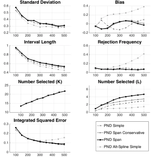
There are noticeable differences in the performance of the estimators. The Span option is able to identify the highest number of relevant covariates, followed by the Conservative Span option, the Simple option, and the Alternative Spline Basis Simple option. The Span, Conservative Span, and Simple Post-Nonparametric Double Selection procedures exhibit favorable finite sample properties for this data generating process. In particular, for those estimators, the calculated rejection frequencies move towards 5% asnincreases.
By contrast, the Alternative Spline Basis Simple Post-Nonparametric Double Selection procedure has very poor finite sample performance. It is unlikely that the projection of the new orthogonalized basis ontoqLhas a good sparse representation. This causes increased model selection mistakes in the first stage. Unlike in the partially linear model, these mistakes can accumulate to cause more severe bias since the number of first stage selection steps is growing with K. Note that the Alternative Spline Basis estimator has similar performance to the Naive estimator in the first part of the simulation study.
The Span and the Conservative Span options offer an opportunity to potentially add additional robustness. These options select more variables than the Simple option. There is no evidence from this simulation study that using the Span option over-selects conditioning variables to the extent that rejection frequencies become severely distorted or variability increases to an undesirable level.
Figure 3. Simulation Results
This figure presents simulation results for the estimation ofg0andθ0in the cases
n= 100,150, ...,500 withs0= 6 andL=n/2 according to the data generating process described
in the text. Estimates are presented for four Post-Nonparametric Double Selection (PND) estimators, Simple, Span, Conservative Span, and Alternative Spline Simple as described in the text. The first plot shows standard deviation of the respective estimates forθ0. The second plot
shows bias of the estimates forθ0. The third plot shows confidence interval length for estimates
forθ0. The fourth plot shows rejection frequencies under the null forθ0 for a 5% level test. The
fifth plot shows the mean number of series termsKused. The sixth plot shows the mean number of series terms fromLselected. The seventh plot shows root mean integrated squared error forg0. In each plot, the horizontal axis denotes sample sizen. Figures are based on 1000
Figure 4. Simulation Results
This figure presents simulation results for the estimation ofg0andθ0in the cases
n= 100,150, ...,500 withs0= 6 andL= 2naccording to the data generating process described
in the text. Estimates are presented for the four Post-Nonparametric Double Selection (PND) estimators, Simple, Span, Conservative Span, and Alternative Spline Simple as described in the text. The first plot shows standard deviation of the respective estimates forθ0. The second plot
shows bias of the estimates forθ0. The third plot shows confidence interval length for estimates
forθ0. The fourth plot shows rejection frequencies under the null forθ0 for a 5% level test. The
fifth plot shows the mean number of series termsKused. The sixth plot shows the mean number of series terms fromLselected. The seventh plot shows root mean integrated squared error forg0. In each plot, the horizontal axis denotes sample sizen. Figures are based on 1000
Figure 5. Simulation study: g0
This figure depicts the functiong0 used in the simulation study.
Figure 6. Simulation study: joint covariate distribution
This figure depicts the joint distribution betweenxand the firsts0= 6 covariates
as described in the above text. The plots are generated by one sample of size