Computing the Endogenous Mortgage Rate
without Iterations
Yevgeny Goncharov
∗January 8, 2008
Abstract
A number of mortgage prepayment models require a specification of the mortgage rate process. Usually some ad-hoc models are used (e.g., a Treasury yield plus some constant). Recently, a number of papers appeared where authors utilized a mortgage rate implied by the cur-rent yield curve (so called endogenous mortgage rate). However, the existing computational algorithms suffer from the curse of dimension-ality and, consequently, are problematic to use for full scale problems. A computational algorithm, proposed in this paper, does not require iterations. Moreover, the algorithm is tractable in the sense that its complexity is equivalent to the problem of mortgage valuation. The numerical example is based on a PDE computation. An implementa-tion of a Monte Carlo method is also discussed.
1
Introduction
A rate level-payment mortgage at first glance looks like a fixed-coupon bond. However, the cash flow of this mortgage is not certain, as its name may imply. Borrowers might prepay mortgages due to various
reasons (in this case the lender “loses” anticipated interest payments1).
This uncertainty (prepayment option) makes mortgage-based securities riskier than traditional fixed-coupon bonds.
Prepayment models try to predict the borrowers’ prepayment be-havior based on information available to the market. There is still no agreement on the “correct” prepayment model. The major trend on
∗Postal address: Yevgeny Goncharov, Department of Mathematics, Florida State Uni-versity, 202A Love Bldg, Tallahassee, FL. E-mail: [email protected]
1
This might be bad for the mortgage investor (if those payments are higher than the current interest rates can provide) or good (if the situation is the opposite).
Wall Street is to model the prepayment behavior empirically. For ex-ample, the prepayment rates are regressed against some explanatory variables, and the 10-year Treasury yield is often considered as one of the most influential predictors.
If we ask “why 10-year Treasury?” then the most common answer would be that this rate closely tracks the 30-year fixed-rate mortgage rate. So, in fact, the empirical models use some benchmark for the mortgage rate. This idea was implemented in the mortgage-rate based (or MRB for short, see [4]) approach to prepayment modeling. It assumes that the borrowers’ refinancing decision is based mainly on
the comparison of the contract and current (available for
refinanc-ing) mortgage rates (the internet is abundant with “calculators” which based on this comparison, tell one how much one “saves” if he/she refi-nances). If this approach to model refinancing incentive is taken, then
the investor needs to model the mortgage rate to be able to model
the prepayment process in order to price or hedge mortgage-backed securities. This mortgage rate model needs to be in agreement with the mortgage rates implied by the resulting prepayment behavior and the underlying interest rate model (we call such mortgage rate models
endogenous).
In spite of its importance, the problem was not considered in depth in academia until recently. The first general endogenous mortgage rate model under sub-optimal prepayment assumption was developed by Goncharov in [4] and [3], where the endogenous mortgage rate is formulated as a fixed-point of a functional operator. Pliska [9] inves-tigated the problem in a discrete time setting. Goncharov, Okten, and Shah [6] applied randomized quasi Monte Carlo method for the mortgage rate computation. Bhattacharjee and Hayre [1] presented a mortgage rate model (called MOATS model) which in fact is a version of the iteration procedure of the fixed-point mortgage rate problem in Goncharov [4], [3] given a certain “educated” initial guess. This guess
comes from solving an auxiliary mortgage problem over a [30,60]-year
interval where mortgages originated at timet∈[30,60] have maturity
of 60−t years.2 Additionally, the MOATS model actually computes
mortgage rate for interest-only mortgages, not the standard (most pop-ular) 30-year fixed-rate fixed-payment fully amortized mortgage.
In this paper we consider the problem of computing the mortgage rate process under the MRB prepayment assumption (i.e., the refi-nancing decision is governed by comparison of the original and current mortgage rates). In [4], the problem of the endogenous mortgage rate was formulated as a fixed point of some functional operator. In [3] and
2
In general, if the interest rate tree in [1] was propagated to 30×(n+ 1) years (instead of 60 = 30×2 years). The question of how close the MOATS mortgage rate approximates the endogenous mortgage rate is addressed in Goncharov [2].
[6] an iterative algorithm was proposed for computation of the endoge-nous mortgage rate process. This algorithm computes the mortgage rates with the help of iterations on every point on some mesh over the interest rate domain. The new algorithm in this paper is based on finding “level curves” of this operator and approximating the mort-gage rate function with an interpolation of these level curves. With a certain condition on the mortgage rate grid, the algorithm does not require iterations. Finding a level curve requires computation of only two conditional expectations, and the number of level curves equals the number of points on the mortgage rate grid, which is one-dimensional. This is in sharp contrast to the existing algorithm proposed in [3] and [6] where the number of expectations to be computed is the number of points needed to reconstruct the mortgage rate function (surface) over the domain of state factors and is a number growing exponentially with the dimensionality of the problem (the complexity of the Citigroup’s MOATS methodology [1] is of the same order).
Let us emphasize that the algorithm can be applied not only to an MRB specification of the prepayment, but to any other prepayment model. Other models might not have a dependence on the mortgage rate process (as the option-based approach in [7], etc.) and, therefore, computing the endogenous mortgage rate for a specific initial state
is a matter of solving ascalarnon-linear equation (which is a simple
problem given that the valuation method with this model is developed). However, if one wants to compute the mortgage rate as a function of “inputs” (e.g., to know/forcast how the mortgage rate will change) the level curve idea in this paper can simplify the numerical computations. The numerical results in this paper confirms the previous findings on the endogenous mortgage rate in [5] and [6]. The endogenous mort-gage rate function exhibits a highly nonlinear behavior around “com-mon” values of the interest rate. This peculiar behavior is strikingly different from the behavior of empirically modeled mortgage rates. The mortgage rates are generally higher if a substantial refinancing risk is present. The “jump” represents an interest rate region which sepa-rates “low”- and “high”-refinancing risk regions. The MRB assump-tion (i.e., the assumpassump-tion that the refinancing is driven by comparison of the mortgage rates) makes these regions “accented.” This peculiarity of the endogenous mortgage rate function needs further investigation since it affects prepayment modeling and pricing (and hedging) of asso-ciated mortgage securities. The point of future empirical studies might be to answer the question: “what if instead of a benchmark we use an endogenous mortgage rate?” A more accurate model (as opposed to us-ing some long rate as a mortgage rate benchmark) would reduce risks to investors and, consequently, might lower mortgage rates in general. The rest of the paper is organized as follows. In Section 2 we give a general model specification which we consider throughout the paper.
In Section 3 we present the computational algorithm in the case of a one-factor interest rate model. In Section 3.1 we present numerical results and in Section 3.2 we study several interesting properties of the endogenous mortgage rates computed in Section 3.1. We discuss the endogenous mortgage rate in the case of heterogenous borrowers in Section 4. In Section 5 we discuss a multi-factor implementation of our algorithm. In particular, we will see that the complexity of the algorithm is equivalent to the complexity of the fundamental mort-gage valuation problem. This is in strike contrast to the general non-tractability of known algorithms which are based on finding mortgage rates given the state space values. In Section 6 we extend the algo-rithm to the case when the transaction costs are “small” or absent. In this case the procedure requires iterations, but stays “tractable” in the sense that it keeps the complexity of the mortgage valuation prob-lem. We shortly discuss the implementation of Monte Carlo method in Section 7.
2
The Model
2.1
Set-up
We consider the following contract: a borrower takes a loan ofP0
dol-lars at the origination and assumes the obligation to pay scheduled
coupons at fixed rate c continuously for duration T of the contract.
The loan is secured by collateral on some specified real estate prop-erty, which obliges the borrower to make the payments. The borrower has the right to settle his/her obligation and prepay the outstanding principal in a lump sum. The interest on the principal is compounded
according to a contract mortgage ratemt, which is determined at the
origination timet and is fixed for the duration of the contract. Given
that the mortgage is fully amortized (i.e., the loan should be
com-pletely payed off after T years), the outstanding principal for time
s ∈ [t, t+T] can be easily computed and is given by the function
P(s−t, mt) = P
01−e
mt(T−(s−t))
1−emt T (where s−t is the time passed after
the origination).
We assume that at any timet it is possible to invest one unit in a
default-free deposit account at a short-term interest ratertand to
“roll-over” the proceeds until a later timesfor a market value at that time
of e
Rs trθdθ
. This interest rate is modeled as a deterministic
(measur-able) functionr(Xt) of some time-homogenous3Markov process (state
variable) Xt = (Xt1, ..., X
p
t) with the support D ⊂ Rp, i.e., for any
X0∈Dwe haveXt∈Da.s. for anyt >0. In what follows, we require
3We might include the non-time-homogenous case by considering, for example,
X1
the monotonicity of the functionr(x) with respect to the components
ofx. In general, this requirement is desirable but not necessary. It will
make the computation more efficient by allowing to avoid iterations. If one cannot reformulate the problem to satisfy this monotonicity as-sumption then the method does not change conceptually but might require iterations.
We consider the usual information structure described by a
nat-ural filtration of the state process (Ω,F,{F}t≥0, Q). We interpret
{Ft}t≥0 as a model of the flow of public information which is not
borrower-specific. The filtration is an intrinsic feature of the market: this means that all traders have the same information available at any
given time. The mortgage rate processmt should be adapted to the
filtration{Ft}t≥0.
2.2
Specification of prepayment
The prepayment time is modeled as the time of the first jump of a gen-eralized Poisson process (the so-called Cox process). This means that
the probability of prepayment is driven by someFt-intensity processγt.
Intuitively speaking, given that a borrower did not prepay as of time
t, the probability that he/she will prepay over the next “short” time
interval △t is γt△t. Equivalently, given a “large” hypothetical pool
of “homogeneous” borrowers,γt is the rate of prepayment (as a
func-tion of a state of economyFt) in terms of proportion (of the borrowers
staying in this pool at timet) per unit of time. Given this intuition,
the prepayment intensityγtcan be regarded as the prepayment rate.
As we pointed out in the introduction, prepayment modeling is a very complicated problem. Modeling the prepayment rate as a func-tion of a set of observable predictors, we essentially specify the prob-ability of prepayment of some given borrower in a given time interval conditioned on some given economy state. Clearly, this probability de-pends on many factors. It can be the contract and current mortgage rates (the borrower compares them to judge how profitable refinancing would be), interest rate yield curve (e.g., if the market expect the in-terest rate to decrease, then borrowers might be inclined to postpone refinancing), so called media effect (historically low mortgage rates get special attention in media and induce higher refinancing), borrower’s credit rating, education, location, loan-to-value ratio, and many many others. All such predictors, with the exception of mortgage rates, are assumed to be modeled by the state process (7), i.e., they are assumed to be exogenously specified. Thus, for a borrower with a mortgage
orig-inated at timet, his/her prepayment intensity (“prepayment rate”) at
times≥t is assumed to be a function of the state variableXs(which
includes all the information about exogenously specified factors such
mortgage ratems, i.e.,γ
s=γ(Xs, mt, ms).
The prepayment decision in the case of ms > mt (time t being
here an origination time) is not, generally, financially based. There-fore, we forbid the refinancing to a mortgage with a higher mortgage
rate.4 The prepayment might happen due to exogenous reasons only.
Technically it means that the prepayment intensity does not depend
on the current mortgage rate ms in this case. Moreover, we assume
that there are transaction costs associated with the refinancing which are measured in terms of mortgage rates. These conditions imply the following specification of the intensity:
γs:=
½
γ1(Xs, mt, ms) ms< mt+δ
γ2(Xs, mt) ms≥mt+δ (1)
whereδ is the transaction cost in percents and for simplicity is taken
as a constant. Note thatγ2(Xs, mt) has the interpretation of the
in-tensity of prepayment due to exogenous reasons.5 To single out the
dependence on the mortgage rates, for the rest of the paper we hide the
dependence onXs by using the notation γs(mt, ms) for the intensity
process defined in (1).
For the most part of the paper we assume that borrowers are ho-mogenous. That is, the probability of prepayment given some state of economy (the current mortgage rate in our case) is the same across all borrowers. This is known to be not the case in practice and there is an empirical proof of this fact in the form of observed burn-out effects: the total prepayment rate in a pool of mortgages which already expe-rienced a refinancing wave is lower (the pool is “burned-out”) because borrowers who are more likely to refinance did so in the time of the pre-vious refinancing wave. We address the case of heterogenous borrowers in Section 4. The problem of the mortgage rate in the non-homogenous case is easier from the computational point of view because a solution in this case is smoother (as we will see) and, therefore, behaves better. From this point of view, our “simplification” (homogenous borrowers) is indeed only a notational one and can be regarded as an extreme (from a computational viewpoint) case.
4In fact, the prepayment intensity (not refinancing part) might be influenced by higher
mortgage rates because borrowers might try to avoid to prepay (even if this decision is not financially based) if the current mortgage rate is very high. For example, a relocation decision due to a new job offer might be easier to make in the case if a new mortgage would have slightly higher mortgage rate than in the case of significantly higher current mortgage rate. Nevertheless, the prepayment intensity due to exogenous reasons is generally much smaller than the refinancing intensity and this kind of dependence of the prepayment intensity on the “negative” refinancing incentive is negligible. However, if desired, the extension of the algorithm to this case is possible with incorporation of iterations.
5Then the intensity of refinancing is
γ1(Xs, m t , ms )−γ2(Xs, m t ) ifms < mt +δand zero otherwise.
2.3
Mortgage rate equation
It can be shown (see [3]) that the price of the mortgageMt(originated
at timetand having contract mortgage ratemt) can be expressed as
the following expectation:
Mt=P(0, mt) +E tZ+T t ¡ mt−ru¢P(u−t, mt)e − u R s (γθ+rθ)dθ du ¯ ¯ ¯ ¯Xs . (2) To exclude an arbitrage opportunity, the price of the mortgage at the origination should be equal to the initial outstanding principal, i.e.,
Mt=P(0, mt) =P0. Using this fact in equation (2), we obtain
0 =E t+T Z t ¡ mt−ru ¢ P(u−t, mt)e− u R t (γθ(m t ,mθ )+rθ)dθ du ¯ ¯ ¯ ¯Xt , (3) which can be written as
mt= E " t+RT t ruP(u−t, mt)e − u R t (γθ(m t ,mθ )+rθ)dθ du ¯ ¯ ¯ ¯Xt # E " t+RT t P(u−t, mt)e− u R t (γθ(mt,mθ)+rθ)dθ du ¯ ¯ ¯ ¯Xt # . (4)
Thus, using the time-homogeneity of the state processXt, the
mort-gage rate process can be defined asmt =m(X
t), where the function
m(x) is the solution of the following functional equation
m(x) = E " T R 0 ruP(u, m(x))e − u R 0 (γθ(m(x),m(Xθ))+rθ)dθ du ¯ ¯ ¯ ¯X0=x # E " T R 0 P(u, m(x))e− u R 0 (γθ(m(x),m(Xθ))+rθ)dθ du ¯ ¯ ¯ ¯X0=x # . (5) The purpose of this paper is to provide a computationally efficient
3
Solving the Model
Let us define the following operator:
A[f(·)](p, x) := E " T R 0 ruP(u, p)e − u R 0 (γθ(p,f(Xθ))+rθ)dθ du ¯ ¯ ¯ ¯X0=x # E " T R 0 P(u, p)e− u R 0 (γθ(p,f(Xθ))+rθ)dθ du ¯ ¯ ¯ ¯X0=x # , (6) wherep∈R+,x∈D⊂Rn, andf :D−→R+.
Given this definition, equation (5) can be written in an operator form as
m(x) =A[m(·)](m(x), x), x∈D.
In principle, this equation can be solved with iterations (see [6]): given
an iteration function mn(x), the following iteration is defined as a
function
mn+1(x) =A[mn(·)](mn(x), x).6
But let us state an important point: the computation ofmn+1(x) for
even one fixedxrequires the knowledge of the previous iteration
func-tionmn(x) for allx∈D. Therefore, the computation of the iteration
functionmn+1(x) requires computation of A[mn(·)](mn(x), x) for all
x∈ D. In particular, for a fixed p the computation of the function
A[mn(·)](p, x) requires computation of onlytwoexpectations, but the
computation of the functionA[mn(·)](mn(x), x) requires evaluation of
the separate expectations in (6) for eachx(i.e.,mn(x)-specific
expec-tations). Practically it means that the number of expectations to be
computed is twice the number of grid points on the domainD. The
number of points required to approximate a surface (i.e., the
mort-gage rate function overD) grows exponentially with the dimension of
the domain in general. If we multiply this complexity for one itera-tion by the number iteraitera-tions required, then we can easily see that this iteration procedure is problematic to employ for real industrial applications.
An alternative computational approach is proposed in this paper. To illustrate our basic idea in the simplest case possible, in this section we assume that the only stochastic process in the model is the
instan-taneous interest rate rt which is a one-factor diffusion process with
rt ∈ D = (0,∞). In this simple interest rate environment the whole
6
A generalized (with the interest rate tree propagated to 30×(n+ 1) years) ver-sion of MOATS mortgage rate model in [1] can be written as iterations mn+1(x) =
A[mn(·)](mn+1(x), x), where m0(x) is taken as a solution to an auxilary mortgage rate
problem over a [30×n,30×(n+ 1)]-year interval where mortgages originated at time
yield curve is determined by the value ofrt, and thus the mortgage rate
processmtis merely a function of the interest rater
t, i.e.,mt=m(rt).
We assume the monotonicity of the mortgage rate function, i.e.,
m(r1) ≤ m(r2) ifr1 ≤ r2. Together with the specification of the
intensity (1), this implies that a borrower’s prepayment intensity does not depend on the behavior of the mortgage rate function for values of
the interest rate higher thanr∗, where r∗ is the value of the interest
rate at the time when the borrower acquired his/her mortgage. The main computational idea is somewhat similar to considering a Lebesgue instead of Riemann integration. Instead of trying to find the mortgage rate for a given interest rate (as we do in a general iteration idea), we fix a mortgage rate value and try to find an appropriate interest rate value.
Let us fix a mortgage rate grid{mn=m0+n△m}Nn=0, where△m
is some value less than the transaction costδ(depends on a precision
desired),N is a number which gives a desired mortgage rate range, and
m0 is an infimum of the mortgage rate values. In the current set-up
m0 is a solution to thescalarequationm0 = lim
r→0+A[1](m0, r), where
“1” stands for “no refinancing” condition.7
Now, for every mn we find an appropriate interest rate value rn
in turn. Suppose rk, k = 0, ..., n−1, are known. Then we
de-fine men(r), r ≤rn−1 as some interpolation function on known pairs
{(rk, mk)}kn=0−1. Given the choice of△m and the monotonicity of the
mortgage rate function, for any possible monotone extensionm(r) of
e
mn−1(r) beyondrn−1we have an a priori estimatem(r)> mn−δfor
all r > rn−1. This implies an a priori fact that the prepayment
in-tensityγtfor computingrn (that is finding at what interest rate value
the mortgage with the rate mn was originated) does not depend on
the mortgage rate behavior for the interest rate valuesr > rn−1. To
formalize this fact, we define the following function
mn−1(r) :=
½ e
mn−1(r) r≤rn−1 ∞ r≥rn−1
which merely extends men(r) in such a way that the refinancing for
r > rn is excluded.
Given these considerations,rn is found by solving the equation
mn=A[mn−1](mn, r)
forr. We can perform this procedure forn= 1, ..., N, and the
approx-imation of a solution to (5) is taken asmeN(r).
7Computationally, lim
r→0+
A[1](m0, r) would be evaluated using the boundary values of
Note that in this case the number of expectations to be computed is
twice the number of themortgage rategrid points. It is known (see [6]),
that the mortgage rate function exhibits a highly non-linear behavior (the “jump”) around some interest rate value which is in the region of “common” interest rate values (i.e., the “jump” cannot be ignored). This “jump” separates the low and high refinance risk regions. Because of this phenomena, the iteration procedure in [3], [6] needed a fine interest grid or an adaptive grid to deal with the “jump.” Formally, applying the procedure considered in this paper, an adaptive interest
grid is computed naturally as a by-product of the method8 (inverse
values of the uniform mortgage rate grid will be more dense in the region of higher gradient of the mortgage rate function). Additionally, we do not need to do iterations at all!
More impressive advantages of this numerical procedure will be seen in a multi-factor setting (Section 5).
3.1
Numerical Example
In this section we explain the computation of the endogenous rate when the expectations are computed with PDEs. We consider a one-factor CIR interest rate model. Where the interest rate is given by a solution of the following stochastic differential equation
drt=α(µ−rt)ds+σ√rtdWt, rt=r∈(0,∞), (7)
and where Wt is a Brownian motion. We consider the following
pa-rameters for the CIR interest rate model: α = 0.3, µ = 0.07, and
σ= 0.115.
LetU[m(·)](mo, x) and W[m(·)](mo, x) be the numerator and
de-nominator of the righthand side of the operatorA[m(·)](mo, x) in
def-inition (6). For the case we consider here we havex=r. For a given
functionm(·), under some technical conditions (see [3]), these functions
are solutions of the following differential equations:
∂U
∂t +LU−[r+γ(r, mo, m(r))]U+rP(t, mo) = 0, (8)
∂W
∂t +LW −[r+γ(r, mo, m(r))]W+P(t, mo) = 0, (9)
UT(r) = 0, WT(r) = 0, (t, r)∈(0, T)×D, (10)
where operator L is the generator of the CIR diffusion state process
rt,i.e., L:= σ 2r 2 ∂2 ∂r2 +α(µ−r) ∂ ∂r. (11) 8
As we will see in Section 3.1, it is sufficient to have a very coarse mortgage rate grid to have this effect. In this case an adaptive mortgage rate grid might be useful. See the note in Section 3.1.
Therefore, the functionA[m(·)](mo, x) is defined as a ratio of solutions
of PDEs (8) and (9).
Next, we assume the following special case of the prepayment in-tensity function:
γt=
½
γ1, ifm0> mt+δ
γ0, ifm0≤mt+δ, (12)
where γ0, γ1, and δ are constants and represent the intensity of
pre-payment due to exogenous reasons, the intensity of prepre-payment in the case when it is financially justifiable, and the transaction costs of refi-nancing in terms of mortgage percentage.
We assume γ0 = 0, γ1 = 0.65, and δ = 1%. This choice implies
that borrowers check their refinancing opportunities in stochastic time
intervals with an average “waiting” time of 1/γ1 ≈ 1.5 years. They
require about 10% of decrease on their monthly mortgage payments (if we compute these “savings” implied by 1% mortgage rate decrease) to refinance and they do not prepay for exogenous reasons. This speci-fication is somewhat similar to the specispeci-fication of the prepayment in [10], where the prepayment rate, however, was assumed to be governed by the borrower’s liability (the so called option-based approach).
The values for the prepayment and interest rate parameters are rounded values of the equivalent parameters estimated in [10] with the
only exception beingδ, since in [10] the transaction costs are expressed
in percents of the outstanding principal while in our case it is expressed in terms of percents of the mortgage rate.
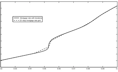
We use a linear interpolation formen(r). The result of the
computa-tion of the endogenous mortgage rate with a 10-step uniform mortgage
rate grid (frommo to 10%) is shown on Fig. (1). As we can see, the
algorithm produces a solution (the dashed line) which tracks closely a “continuous” solution (solid line) computed with iterations (which are
computed forevery point on the interest grid). The exception is the
“jump” region where the deviation from the “continuous” solution is due to the linear interpolation.
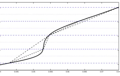
In Fig. 2 we magnify the region of the “jump” and show the mort-gage rate function computed with our algorithm with 5 (dash-dotted line), 10 (dashed line), and 20 (dotted line) steps of the uniform mort-gage rate grid. The appropriate horizontal lines (dash-dotted, dashed, or dotted according the number of steps used) shows the levels of the mortgage rates used to compute the corresponding interest rates. The mortgage rate solution computed with 40 step mortgage rate grid is visually indistinguishable from the “continuous” solution.
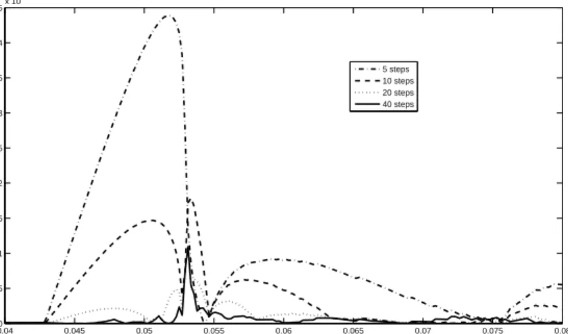
Fig. 3 shows the absolute value of the deviation of the level set solutions form the “continuous” mortgage rate function. All grids pro-duce the mortgage rate functions which are practically indistinguish-able from the “continuous” solution for the small interest values (a half
0.02 0.03 0.04 0.05 0.06 0.07 0.08 0.09 0.1 0.05 0.055 0.06 0.065 0.07 0.075 0.08 0.085 0.09 0.095 0.1
Mortgage rate with iterations 10−step mortgage rate grid
interest rate
mortgage rate
Figure 1:
Comparison of the mortgage rate function computed with iterations at every point of the interest rate grid (solid line) and the mortgage rate function computed with 10 steps mortgage rate grid (dashed line).of a percentage point for 5 step grid and less than a quarter of a point for other grids for the interest rate values less than 4%). We can see that large deviations for 5 and 10 step mortgage rate grids are due to points of linear interpolations. For 20 step grid the errors are less than 2.5 basis points except for the neighborhood of the “jump.” For the 40 step grid the errors are around of one basis point. The only exclusion is a narrow neighborhood (plus/minus 10 basis points of the “jump” location) of the “jump” where the high gradient makes the deviation to be around 10 basis points.
Note on adaptive grid. As we see in Fig. 2 and Fig. 3, the er-ror is negligible for the interest rate values to the left of the “jump.” Around the “jump” the linear interpolation is not adequate for large
△m, though the values of the mortgage rates at points which
corre-spond to the mortgage rate level values (mn for rn in our notation)
were very close in either case (less then a half of a point even in 5 or 10 step case). This suggests the following idea for an adaptive mesh.
Assume the mortgage rate function for values lower thenmn is found
(i.e.,m(r) is approximated forr≤rn). We take a large mortgage rate
step, say,△mn+1=δand compute the interest ratern+1 for the level
mn+△m. Then we take a half step, i.e., we compute the interest rate
rn+1/2 for the levelmn+△m/2. Now ifmn+△m/2 is within some
0.04 0.045 0.05 0.055 0.06 0.065 0.07 0.075 0.06 0.065 0.07 0.075 0.08
Figure 2: Level sets for the algorithm with 5, 10, and 20 step mortgage rate
grids.
approximation of the mortgage rate function for the interest rate
val-uesr≤rn+1, otherwise we divide the intervals (m
n, mn+△m/2) and
(mn+△m/2, mn+△m) further in half and check ifrn+1/4andrn+3/4
are satisfactorily close to the interpolation with the “inserted” point
rn+1/2, etc.
3.2
On some qualitative properties.
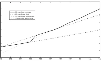
As we pointed out, if the mortgage rate process is needed for certain purposes, then a common practice is to take some long-term Treasury yield as a benchmark for the mortgage rate (e.g., the mortgage rate process is modeled as the 10-year Treasury yield plus some exogenously specified constant). If we look at the endogenous mortgage rate (Fig. 1) then we can see that its non-linear behavior (e.g., the “jump” around 5.5% and the “hump” around 9%) does not allow a satisfactory uniform fit for any Treasury yield. Let us take a Treasury yield as a function of the initial short interest rate (which uniquely specifies the current yield curve in our one-factor CIR interest rate model setting) and pick a term which “fits” the endogenous mortgage rate only on some interval of the interest rate values. As we can see on Fig. 4, we can separate three regions: 1) on the left to the “jump” (the interest rates less than around 5.5%) the 30-year Treasury fits the mortgage rate; 2) the 10-year Treasury is close to the mortgage rates between the “jump” and the “hump” (the interest rates between around 5.5% and 8%); 3) the
0.040 0.045 0.05 0.055 0.06 0.065 0.07 0.075 0.08 0.5 1 1.5 2 2.5 3 3.5 4 4.5x 10 −3 5 steps 10 steps 20 steps 40 steps
Figure 3: Deviations of the solutions based on the 5, 10, 20, and 40 step
grids from the mortgage rate function computed with iterations for every
point on the interest rate grid.
5-year Treasury gives a good fit after the “hump” (the interest rates larger than around 8%). On Fig. 4, we added appropriate constants to 5- and 10-year Treasury yields to get the “fit”.
This simple experiment illustrates why 10-year Treasury yield might work nicely in certain circumstances. Let us emphasize that this fit is a purely ad-hoc approach and in different economic situations differ-ent terms might be required to be used as benchmarks to have a good performance. Additionally, any such benchmark ignores the presence
of the “jump.”9
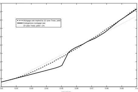
Let us see what mortgage rate we get if the prepayment model is based on the 10-year Treasury yield benchmark (i.e., one version of a simple empirical prepayment model). Assume that the refinancing decision is triggered by the 10-year Treasury yield, i.e., the prepayment
rate is specified as10
γt=
½
γ1, ify10(r0)> y10(rt) +δ
γ0, ify10(r0)≤y10(rt) +δ (13)
9As we will show in the next section, the “jump” is smoothed out in the more realistic
case of heterogenous borrowers. However, the transaction between the lower and higher interest rate region is still present and cannot be ignored.
10
Compare with the definition of the intensity (12) where the refinancing decision is driven by the endogenous mortgage rate.
0.02 0.03 0.04 0.05 0.06 0.07 0.08 0.09 0.1 0.11 0.12 0.04 0.05 0.06 0.07 0.08 0.09 0.1 0.11 0.12
30−year fixed mort. rate 30−year Treas. yield 10−year Treas. yield + const. 5−year Treas. yield + const.
Figure 4: Comparison of the mortgage rates and certain Treasury yields as
functions of the short interest rate.
wherey10(r) is the 10-year Treasury yield given that the current
inter-est rate isr.Fig. 5 shows the comparison of the mortgage rates implied
by this empirical model (dashed line) and the endogenous mortgage rates (solid line). The mortgage rate implied by the 10-year Trea-sury yield grossly overestimates the endogenous mortgage rate for the interest rates to the left of the jump.
An explanation of the significantly lower endogenous values is that the lenders giving the lower mortgage rates for borrowers would be compensated by the virtual absence of the refinancing in lower rate situations in the presence of the 1% transaction costs. However, the risk of refinancing is significant if the mortgage rates are given using the 10-year Treasury benchmark.
This compensation (i.e., reduction of the refinancing risk) is not enough for the interest rates higher than around 5.5%. Between 5.5% and 6.5% the 10-year Treasury benchmark implies lower (of about 10 basis points) mortgage rates. In this case the empirical model un-derestimates the refinancing risk (which is presented by the “jump”). Between 7% and 8.5% the 10-year Treasury benchmark implies higher (about 10 basis points) mortgage rates. In this case the refinancing risk predicted by the endogenous mortgage rate process is lower because of
the higher endogenous mortgage rates in the (5.5%,6.5%) interest rate
region and, consequently, the lower refinancing incentivem(r0)−m(rt)
there.
0.01 0.02 0.03 0.04 0.05 0.06 0.07 0.08 0.09 0.1 0.05 0.055 0.06 0.065 0.07 0.075 0.08 0.085 0.09 0.095 0.1
Mortgage rate implied by 10−year Treas. yield Endogenous mortgage rate
10−year Treas. yield + 1%
interest rate
mortgage rate
Figure 5: Comparison of the endogenous mortgage rates with the 10-year
Treasury yield benchmark and the mortgage rates implied by the
prepay-ment model which is based on this benchmark.
mortgage rate implied by the 10-year Treasury benchmark is not a
solution to the mortgage rate equation equation (5). Compare the mortgage rate implied by this benchmark with the 10-year Treasury yield itself. In Fig. 4 we “attempt” to fit the 10-year Treasury to the implied mortgage rate by adding 1% to the yield. The slope of the implied mortgage rate function is about the same for interest rates between 3% and 5% but significantly higher for higher interest rates. That is, the prepayment models which use the 10-year Treasury bench-mark for the mortgage rate modeling are not arbitrage free.
4
Heterogenous Borrowers
In this section we illustrate the extension of our framework to the case of pools with heterogenous borrowers. Assume the set of all possible borrower’s intensity functions is given by the parameterized family
{γω
t}ω∈Ω. Next, we assume that we have statistically estimated the
distribution Φω of borrowers in some geographical region where the
mortgage rate model are to be used. Then the distribution of borrowers in a pool which is just originated in that geographical region can be
viewed as an unbiased estimator of Φω. The deviation of the actual
borrowers distribution in the pool from Φωrepresents the idiosyncratic
risk for investors and should not be priced. Taking this into account and repeating the manipulations of section 2.3, we conclude that the mortgage rate is given by the equation
m(x) = R Ω E " T R 0 ruP(u, m(x))e − u R 0 (γω θ(m(x),m(Xθ))+rθ)dθ du ¯ ¯ ¯ ¯Xt=x # dΦω R Ω E " T R 0 P(u, m(x))e− u R 0 (γω θ(m(x),m(Xθ))+rθ)dθ du ¯ ¯ ¯ ¯Xt=x # dΦω . (14)
The computation of the Φω-integral might be evaluated with the
help of some quadrature if Φωis a sufficiently smooth distribution.
In Fig. 6 we illustrate a solution to this equation assuming that all the borrowers can be divided into three (with equal proportions) groups: 0.7% transaction costs, 1% transaction costs, and 1.3% trans-action costs. The other parameters are taken to be the same as in Section 3.1. 0 0.02 0.04 0.06 0.08 0.1 0.12 0.05 0.06 0.07 0.08 0.09 0.1 0.11 interest rate mortgage rate
Effects of Transaction Costs
TC = 0.007 TC = 0.01 TC = 0.013 pool
Figure 6: The mortgage rate in the case of heterogenous borrowers.
As we can see, in the presence of heterogenous borrowers the “jump” region is smoothed out. From the computational point of view it means that the interpolation between level curves is going to be closer in this (more realistic!) case. In particular, the step size of the mortgage rate
mesh△mmight be taken larger (without losing the precision) than in the case of homogenous borrowers.
5
Multi-factor Extension
As we pointed out, iteration procedures, which are based on finding the mortgage rates for given interest rate values, suffer from a curse of di-mensionality. Let us emphasize that this is a problem of the procedure itself and not of the expectations computation. Additionally, proce-dures of “consecutive” iterations in [3] and [6] is problematic to extend to multi-dimensional models because a space of dimension greater than one is not ordered (see [6]). But with the procedure considered in this paper, the extension to higher dimensions is natural. Moreover, the number of the expectations to be computed in this algorithm does not grow with the dimensionality of the state process. This is a seri-ous advantage over iteration procedures where we have an exponential growth (with respect to the state process dimension) in the number of expectation computations.
Assume that the interest rate process rt = r(Xt) is a function of
the p-dimensional state process Xt ∈ Rn. We discretize the
(one-dimensional!) values of the mortgage ratesmn, n= 0, ..., N, the same
way we did in the one-factor case.11 Now, consider the equation
m1=A[1](m1, x),
wherex∈Rp and the constant function 1 stands for “no refinancing”
condition. The solution of this equation is a manifoldl1ofA[1](m1, x)
as function ofx. We will refer to this solution as a “level curve”, i.e.,
as if p = 2. Given the monotonicity of the mortgage rate function
m(x) with respect to the components of x, this level curve separates
the region (in terms of x) of higher and lower (than m1) mortgage
rates. Let us use notationL1for the lower mortgage rate domain, i.e.,
L1 = {x| m(x) < m1}. The borrowers who receive their mortgages
in the situation when the yield curve implies that the state variable is from this domain will never refinance their mortgages because for any
Xt∈L1we havem(Xt)> m1−δ(according to the way the mortgage
rate grid is defined) and for anyXt∈ D\L1 we have m(Xt) > m1.
The approximation of the mortgage rate overL1 can be defined as an
interpolation betweenm0 andm1 onl1.
Before we proceed, let us formulate the major idea. A given level
curveln (being defined below) defines the boundary of the domain of
dependence Ln for the mortgages originated on this level curve (the
mortgage rates are higher “outside” ofln, i.e., whereXt∈D\Ln, and
11
do not influence the prepayment decision). Therefore, the operatorA
for findingln+1(i.e., for mortgages originated onln+1) will depend only
on domainLn, where the mortgage rate function can be approximated
by an interpolation on the level curves lk, k = 0, ..., n. Therefore,
finding the level curvesln consecutively forn= 1, ..., N, we construct
an approximation of the mortgage rate function by an interpolation on these level curves.
Let us assume that the level the curveslk fork = 1, ..., n−1 are
known. Similarly to the one-factor case, we define men−1(x) as an
interpolation between the known level curveslk. Next, we define
mn−1(x) :=
½ e
mn−1(x) x∈Ln−1 ∞ x6∈Ln−1
Then the level curvelnis defined as a solution to the following equation
mn=A[mn−1](mn, x). (15)
As we see, in the multi-factor case the number of equations to be solved is the same as in the one-factor case (since in either case we
discretize the one-dimensional mortgage rate space). The growth of
complexity comes from the computation of expectations and finding level curves only. The problem of finding a level curve is computa-tionally cheaper then evaluating the conditional expectations in the
definition of the operator Aitself. At the same time, the
computa-tion of these expectacomputa-tions has equivalent complexity to evaluating the fundamental problem of computing the mortgage price (compare the
mortgage price equation (2) to the definition (6) of the operatorA).
It means that if one implements an empirical multi-factor mortgage model, then the computational complexity of including an endogenous mortgage rate instead of its benchmark can be practically implemented too.
6
Extension to zero transaction cost
If the transaction costδis small, then the mortgage rate grid might be
unnecessarily fine because of our requirement△m≤δ. If we assume
zero transaction cost, than the procedure does not work the way it was
described (△m = 0 does not make sense). But the algorithm can be
extended to overcome this complication.
Let us assume we are given the level curves lk, k = 1, ..., n−1,
and want to define the level curveln, i.e., to find values of the interest
rates which imply the mortgage rate mn. First, we take an initial
guess l0
n such that l0n 6⊂ Ln−1 (otherwise, the mortgage rate surface
extrapolation of previous level curves{lk}1n−1. Then we defineme0n(x)
as an interpolation between the known level curveslk plus our initial
guessl0 n. Next, define m0 n(x) := ½ e m0 n(x) x∈L0n ∞ x6∈L0 n whereL0
nis the region “inside”l0n. To findlnwe use iterations. Given
an iteration level curveli
n, the mortgage rate functionmin(x) is defined
in a similar fashion asm0n(x). Iteration level curveslin themselves are
defined iteratively as solutions to
mn=A[min−1](mn, x), i= 1,2, ...
In this case we have to run iterations but the complexity of the procedure still stays independent of the dimension of the state process
(without regard to computation of expectations in A), which makes
the procedure more promising than the iteration procedures based on the computation of the mortgage rates given fixed interest rate values.
7
Note on Monte-Carlo Implementation
Although the complexity of the numerical procedure by itself, as we’ve seen, does not grow with the dimension of the state process, the prob-lem of dimensionality might appear in the valuation of expectations itself. PDE approach, illustrated in Section 3.1, can be easily imple-mented in a one-factor setting. It is feasible to implement the same framework in the case two- or three-dimensional state processes. How-ever, for higher dimensions the problem of the “curse of dimensional-ity” might make the problem computationally too hard.
To overcome the curse of dimensionality, one might want to use Monte Carlo simulation. Additionally, Monte Carlo method has a very important advantage for practitioners in the sense that one could very easily implement different kinds of interest rate models (e.g., jump-diffusion). However a “straightforward” Monte Carlo implementation implies computation of expectations at one given point (initial position of the state process), while for our iterative procedure we need to know the “whole” conditional expectation to find an appropriate level
curve.12
The answer to this problem can be given by regression techniques which were used for Monte Carlo estimation of the optimal stopping time for American options pricing in [12], [11], [8]. The idea is based
on the fact that conditional expectations from the L2 space can be
12Or at least, we should know the conditional expectation in some domain which would
represented by a linear combination of functions from acountable basis
in this space (sinceL2is a Hilbert space). In practice, the expectations
are approximated by a finite number of these basis functions.
References
[1] Bhattacharjee, R., and L.S. Hayre,The Term Structure of
Mort-gage Rates: Citigroup’s MOATS Model,Journal of Fixed Income,
March 2006.
[2] Goncharov, Y., On convergence of MOATS to endogenous
mort-gage rate proces,working paper, 2008.
[3] Goncharov, Y., An Intensity-Based Approach to the Valuation of
Mortgage Contracts and Computation of the Endogenous
Mort-gage Rate, International Journal of Theoretical and Applied
Fi-nance, Vol. 9, pp. 889-914, 2006.
[4] Goncharov, Y., Mathematical Theory of Mortgage Modeling,
Ph.D. dissertation, University of Illinois at Chicago, 2003.
[5] Goncharov, Y., On the Mortgage Rates Implied by the
Option-Based and Empirical Approaches,proceedings of Hawaii
Interna-tional Conference on Statistics, Honolulu, 2004.
[6] Goncharov, Y., Okten, G., and M. Shah,Computation of the
En-dogenous Mortgage Rates with Randomized Quasi-Monte Carlo
Simulations, Mathematical and Computer Modelling, in press,
available on elsevier.com.
[7] Kalotay, A., Young, D., and F. Fabozzi, An option-theoretic
pre-payment model for mortgages and mortgage-backed securities,
In-ternational Journal of Theoretical and Applied Finance, 7(8): 1-29, 2004.
[8] Longstaff F., Schwartz E. Valuing American options by
simula-tion: a simple least squares approachReview of Financial Studies,
14:113–147, 2001.
[9] Pliska, S.,Mortgage Valuation and Optimal Refinancing,
Proceed-ings of Stochastic Finance 2004, Lisbon, Portugal (Springer Ver-lag).
[10] Stanton, R.,Rational prepayment and the valuation of
mortgage-backed securities, Review of Financial Studies, 8: 677-708, 1995.
[11] Carriere, J.,Valuation of Early-Exercise Price of Options Using
Simulations and Nonparametric Regression, Insurance:
Mathe-matics and Economic, 19, pp. 19–30, 1996.
[12] Tsitsiklis, J., and Van Roy, B.,Optimal Stopping of Markov
Application to Pricing High-Dimensional Financial Derivatives, IEEE Transactions on Automatic Control, 44(10), pp. 1840–1851, 1999.