Lin Chen
Submitted in partial fulfillment of the requirements for the degree of
Doctor of Philosophy under the Executive Committee of the Graduate School of Arts and Sciences
COLUMBIA UNIVERSITY
Lin Chen
Continuous-Time and Distributionally Robust Mean-Variance Models Lin Chen
This thesis contains three works in both continuous-time and distributionally robust mean-variance Markowitz models. In the first work, we study naive
strategies in the continuous-time mean-variance model. We propose a new type of agent to approximate the dynamic of the naive agent by partitioning the time line into numerous small equal length time intervals. Then, we prove that, the wealth process of the proposed agent converges to that of the naive agent and derive the explicit formula for the limiting wealth process and its corresponding portfolio process. In the end, we compare the naive strategies with two equilibrium strategies in the Black-Scholes market.
The second work contributes to the mean-variance model by considering its distributionally robust counterpart, where the region of distributional uncertainty is around the empirical measure and the discrepancy between probability measures is dictated by the Wasserstein distance. We reduce this problem to an empirical variance minimization problem with an additional regularization term. Moreover, we extend the recently developed inference methodology to our setting in order to select the size of the distributional uncertainty as well as the associated robust target return rate in a data-driven way. Finally, we report extensive backtesting results on the S&P 500 that compares the performance of our model with those of several well-known models, including the Fama–French model and the
In the last part, we develop a distributionally robust model based on the Sharpe ratio optimization problem. We transform the problem into an equivalent convex optimization problem that can be solved numerically. In this model, we do not need to choose the target return parameter, which has to be decided by
subjective judgement in previous distributionally robust mean-variance models. As a result, the distributionally robust Sharpe ratio model is completely data-driven. We also provide guidance on the choice of ambiguity set size by using a much simpler scheme than that employed in the second work. In the end, we compare the performance of this model to that of the second work and some other well-known models on S&P500.
List of Figures iii
Acknowledgments x
1 Introduction 1
1.1 The Classical Single-Period Mean-Variance Markowitz Model . . . 1
1.2 Multi-Period and Continuous-Time MV Models and Time-Inconsistency 2 1.3 Robust MV Models . . . 4
1.4 Main Contributions of This Thesis . . . 9
1.4.1 Naive Strategies in a Continuous-Time MV Model . . . 9
1.4.2 A Distributionally Robust Mean-Variance Model . . . 11
1.4.3 A Distributionally Robust Sharpe Ratio Model . . . 14
1.5 Organization of the Thesis . . . 15
2 Naive Strategies in Continuous-Time MV Model 17 2.1 Problem Formulation . . . 17
2.1.1 Continuous-Time Market . . . 17
2.1.2 Continuous-Time Mean-Variance Model . . . 19
2.2 Strategies of a Naive Agent . . . 21
2.2.1 Time-Inconsistency and the Naive Agent . . . 21
2.2.2 2n-committed Agent . . . . 24
2.3 Naive Strategies and Equilibrium Strategies . . . 38
2.3.2 The case γ(x) = x . . . 41
2.3.3 The case L(t, x) = xek(T−t) . . . 44
2.4 Conclusions . . . 46
3 A DRMV Model 48 3.1 Model Formulation . . . 48
3.2 Transformations, Duality, and Regularization . . . 50
3.3 Choice of Model Parameters . . . 61
3.3.1 Choice ofδ . . . 62
3.3.2 Choice of ¯α . . . 71
3.4 Empirical Performance and Comparisons . . . 73
3.4.1 Experiment Design and Data Preparation . . . 74
3.4.2 Comparisons . . . 80
3.4.3 Discussion . . . 86
3.5 Concluding Remarks . . . 96
4 A DRSR Model 97 4.1 Model Formulation . . . 97
4.2 Transformations and Tractability . . . 100
4.3 Choice of Model Parameter δ . . . 110
4.4 Empirical Performance and Comparisons . . . 120
4.4.1 Experiment Design and Data Preparation . . . 120
4.4.2 Comparisons . . . 124
4.5 Concluding Remarks . . . 128
Bibliography 135
2.1 This graph shows two sample paths of wealth processes. The blue dashed line represents the wealth process corresponding to the opti-mal portfolio obtained at time 0. The red line is the wealth process corresponding to the optimal portfolio obtained at timet. . . 23 2.2 This figure shows one sample path of wealth process Xn(s). Each
different color shows the wealth process corresponding to the optimal portfolio obtained at time tk, k = 0,1, ...,2n−1. The process is
con-tinuous. . . 24
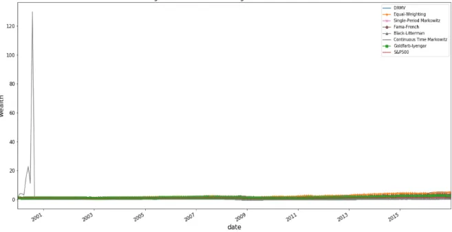
3.1 This graph presents the wealth processes of all portfolios (including continuous-time Markowitz) and the S&P 500 from January 2000 to December 2016. All of the portfolios except S&P 500 consist of 100 stocks, and the averages are calculated over 100 numerical experiments. Thex-axis indicates the time in months (from 1 to 204) and they-axis indicates the portfolio wealth. Initial wealth is set at 1. . . 80 3.2 This graph presents the wealth processes of all portfolios (excluding
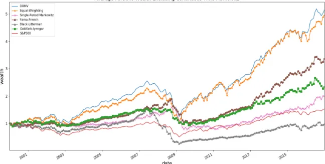
continuous-time Markowitz) and of the S&P 500 from January 2000 to December 2016. All of the portfolios except the S&P 500 consist of 100 stocks, and the averages are calculated over 100 numerical experiments. Thex-axis indicates the time in months (from 1 to 204) and they-axis indicates the portfolio wealth. Initial wealth is set to be 1. . . 82
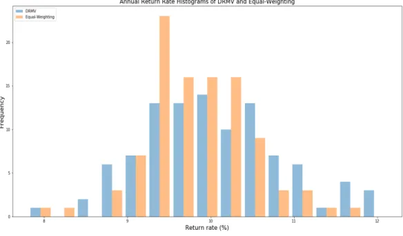
100 different experiments on the DRMV (blue) and equal-weighting (orange) portfolios. The x-axis represents the annualized returns and the y-axis represents the number of returns. . . 83 3.4 This graph presents the histograms of the Sharpe ratio of the 100
dif-ferent experiments on the DRMV (blue) and equal-weighting (orange) portfolios. The x-axis represents the Sharpe ratio and the y-axis rep-resents the number of Sharpe ratios. . . 83 3.5 This graph presents the histograms of the kurtosises of the 100
dif-ferent experiments on the DRMV (blue) and equal-weighting (orange) portfolios. Thex-axis represents the kurtosis and they-axis represents the number of kurtosises. . . 84 3.6 This graph presents the histograms of the annualized returns of the
100 different experiments on DRMV (blue) and Fama-French (orange) portfolios. Thex-axis represents the annualized returns and they-axis represents the numbers of returns. . . 85 3.7 This graph presents the histograms of the Sharpe ratio of the 100
dif-ferent experiments on the DRMV (blue) and Fama-French (orange) portfolios. The x-axis represents the Sharpe ratio and the y-axis rep-resents the number of Sharpe ratios. . . 85 3.8 This graph presents the histograms of the kurtosises of the 100
dif-ferent experiments on the DRMV (blue) and Fama-French (orange) portfolios. Thex-axis represents the kurtosis and they-axis represents the number of kurtosises. . . 86
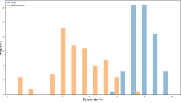
100 different experiments on the DRMV (blue) and Goldfarb–Iyengar (orange) portfolios. There are two experiments in which Goldfarb-Iyengar went into bankruptcy, which are not included in this histogram. Thex-axis represents the annualized returns and the y-axis represents the number of returns. . . 87 3.10 This graph presents the histograms of the Sharpe ratios of the 100
different experiments on the DRMV (blue) and Goldfarb–Iyengar (or-ange) portfolios. Thex-axis represents the Sharpe ratios and they-axis represents the number of Sharpe ratios. . . 88 3.11 This graph presents the histograms of the kurtosises of the 100
differ-ent experimdiffer-ents on the DRMV (blue) and Goldfarb–Iyengar (orange) portfolios. Thex-axis represents the kurtosis and they-axis represents the number of kurtosises. . . 88 3.12 This graph presents the histograms of the annualized returns of the 100
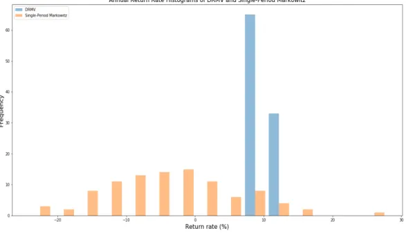
different experiments on the DRMV (blue) and single-period Markowitz (orange) portfolios. The x-axis represents the annualized returns and the y-axis represents the number of returns. . . 89 3.13 This graph presents the histograms of the Sharpe ratios of the 100
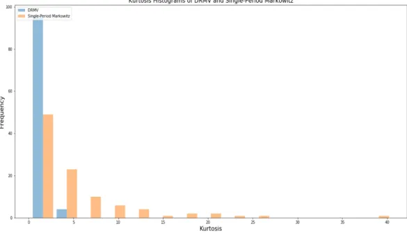
dif-ferent experiments on the DRMV (blue) and single-period Markowitz (orange) portfolios. The x-axis represents the Sharpe ratios and the y-axis represents the number of Sharpe ratios. . . 90 3.14 This graph presents the histograms of the kurtosises of the 100
dif-ferent experiments on the DRMV (blue) and single-period Markowitz (orange) portfolios. The x-axis represents the kurtosis and the y-axis represents the number of kurtosises. . . 90
100 different experiments on the DRMV (blue) and Black–Litterman (orange) portfolios. The x-axis represents the annualized returns and the y-axis represents the number of returns. . . 91 3.16 This graph presents the histograms of the Sharpe ratios of the 100
different experiments on the DRMV (blue) and Black–Litterman (or-ange) portfolios. Thex-axis represents the Sharpe ratios and they-axis represents the number of Sharpe ratios. . . 92 3.17 This graph presents the histograms of the kurtosises of the 100
differ-ent experimdiffer-ents on the DRMV (blue) and Black–Litterman (orange) portfolios. Thex-axis represents the kurtosis and they-axis represents the number of kurtosises. . . 92 3.18 This graph presents the portfolio average wealth processes of DRMV
(p= 2) and DRMV-p1 (p= 1) from January 2000 to December 2016. The averages are calculated over 100 numerical experiments. The x-axis indicates the time and the y-axis indicates the portfolio wealth. Initial wealth is set at 1. . . 93 3.19 This graph presents DRMV’s average wealth processes from January
2000 to December 2016 with different values of ρ. The averages are calculated over 100 numerical experiments. The x-axis indicates the time and they-axis indicates the portfolio wealth. Initial wealth is set at 1. . . 93 3.20 This graph presents the histogram of the DRMV monthly turnover
rates of 100 experiments. Thex-axis represents the turnover rate (%) and they-axis represents the numbers of turnover rates. . . 94
age estimators from January 2000 to December 2016. All the portfo-lios except S&P 500 consist of 100 stocks and the averages are calcu-lated over 100 numerical experiments. Thex-axis indicates the time in months (from 1 to 204) and the y-axis indicates the portfolio wealth. Initial wealth is set to be 1. . . 95
4.1 This graph presents the wealth processes of all portfolios (allow short-selling) and of the S&P 500 from January 2000 to December 2016. All of the portfolios except the S&P 500 consist of 100 stocks, and the averages are calculated over 100 numerical experiments. The x-axis indicates the time in months (from 1 to 204) and the y-axis indicates the portfolio wealth. Initial wealth is set at 1. . . 124 4.2 This graph presents the wealth processes of all portfolios (allow
short-selling and without classical Sharpe ratio and Fama-French model) and of the S&P 500 from January 2000 to December 2016. All the portfolios except the S&P 500 consist of 100 stocks, and the averages are calculated over 100 numerical experiments. The x-axis indicates the time in months (from 1 to 204) and they-axis indicates the portfolio wealth. Initial wealth is set at 1. . . 125 4.3 This graph presents the wealth processes of all portfolios (NOT
allow-ing short-sellallow-ing) and of the S&P 500 from January 2000 to December 2016. All the portfolios except S&P 500 consist of 100 stocks, and the averages are calculated over 100 numerical experiments. The x-axis indicates the time in months (from 1 to 204) and the y-axis indicates the portfolio wealth. Initial wealth is set at 1. . . 127
different experiments on the DRSR (blue) and classical Sharpe ratio (orange) portfolios. The x-axis represents the annualized return and the y-axis represents the number of returns. . . 127 4.5 This graph presents the histograms of the Sharpe ratio of the 100
different experiments on the DRSR (blue) and classical Sharpe ratio (orange) portfolios. The x-axis represents the Sharpe ratio and the y-axis represents the number of Sharpe ratios. . . 128 4.6 This graph presents the histograms of the annualized returns of the 100
different experiments on the DRSR (blue) and single-period Markovitz (orange) portfolios. The x-axis represents the annualized return and the y-axis represents the number of returns. . . 129 4.7 This graph presents the histograms of the Sharpe ratio of the 100
different experiments on the DRSR (blue) and single-period Markovitz (orange) portfolios. The x-axis represents the Sharpe ratio and the y-axis represents the number of Sharpe ratios. . . 130 4.8 This graph presents the histograms of the annualized returns of the
100 different experiments on the DRSR (blue) and Black-Litterman (orange) portfolios. The x-axis represents the annualized return and the y-axis represents the number of returns. . . 131 4.9 This graph presents the histograms of the Sharpe ratio of the 100
dif-ferent experiments on the DRSR (blue) and Black-Litterman (orange) portfolios. The x-axis represents the Sharpe ratio and the y-axis rep-resents the number of Sharpe ratios. . . 131 4.10 This graph presents the histograms of the annualized returns of the 100
different experiments on the DRSR (blue) and Fama-French (orange) portfolios. The x-axis represents the annualized return and the y-axis represents the number of returns. . . 132
different experiments on the DRSR (blue) and Fama-French (orange) portfolios. The x-axis represents the Sharpe ratio and the y-axis rep-resents the number of Sharpe ratios. . . 132 4.12 This graph presents the histograms of the annualized returns of the
100 different experiments on the DRSR (blue) and DRMV (orange) portfolios. The x-axis represents the annualized return and the y-axis represents the number of returns. . . 133 4.13 This graph presents the histograms of the Sharpe ratio of the 100
differ-ent experimdiffer-ents on the DRSR (blue) and DRMV (orange) portfolios. The x-axis represents the Sharpe ratio and the y-axis represents the number of Sharpe ratios. . . 133 4.14 This graph presents the histograms of the annualized returns of the
100 different experiments on the DRSR (blue) and equal-weighting (orange) portfolios. The x-axis represents the annualized return and the y-axis represents the number of returns. . . 134 4.15 This graph presents the histograms of the Sharpe ratio of the 100
dif-ferent experiments on the DRSR (blue) and equal-weighting (orange) portfolios. The x-axis represents the Sharpe ratio and the y-axis rep-resents the number of Sharpe ratios. . . 134
This thesis concludes my five years of doctoral study and research efforts. In the course of my Ph.D. life, I have become deeply indebted to many excellent scholars and exceptional individuals.
First and foremost, I would like to thank my advisor, Professor Xunyu Zhou, for his careful and enlighting guidance. He is a talented researcher and an insightful mentor. It has been a great honor for me to work with him closely over the course of my Ph.D. career. He came to Columbia University in the second year of my Ph.D. process, and he gave me the confidence and support that put me on the right track. I will always remember lots of precious moments when I went to his office and discussed problems with him using the whiteboard. He has taught me how to be a good researcher and, even more importantly, how to be a good person.
Besides my advisor, I would like to thank the rest of my thesis committee, Pro-fessor Agostino Capponi, ProPro-fessor David Yao, ProPro-fessor Henry Lam, and ProPro-fessor Paul Glasserman, for generously offering their precious time to serve on my defense committee and for providing invaluable advice. Also, I want to thank Professor Jose Blanchet, with whom I collaborated along with Professor Zhou on the work of Chap-ters 3 and 4. I also want to thank Professor Jing Dong, with whom I worked on another research project about exact sampling of the maximum of the Gaussian Pro-cesses with infinite memory. I really appreciate the guidance and kind help of these two scholars, as well as my committee members.
I am also grateful to many friends and colleagues whom I have I met over the past
during my Ph.D. process: Wei You, Di Xiao, Brian Ward, Cun Mu, Fei He, Chaoxu Zhou. Also, I want to thank the members of my academic family, Professor Xuedong He, Professor Hanqing Jin, Professor Sang Hu, Xiao Xu, and Yilie Huang. I also thank my fellow Ph.D. students, Fengpei Li, Yunjie Sun, Weilong Fu, Yi Ren, Yan Chen, Wenjun Wang, Yunhao Tang, Jingtong Zhao, Raghav Singal, Kumar Goutam, Randy Jia, as well as my friends out of the IEOR department, Yiwen Shen, Weizhuo Sun, Zhongyi Zhang, Xun Wang, Qiliang Lin, Siyu Zhu, Yanru Chen, Tianyang Zhang and Dawei Zhang. Thanks also to all of my friends, this journey has been exciting and enjoyable with your company, and I will always cherish the memories of us attending courses, discussing problems, talking, and laughing together.
I thank my advisor, Columbia University, and the CKGSB doctoral fellowship program for their generous financial support.
Lastly and most importantly, I owe my deepest gratitude to my parents, Yonggang Chen and Lifang Xian, and to my wife, Sixia Su, for their unconditional love and endless support throughout my life. Their faith in me has always encouraged me.
Introduction
1.1
The Classical Single-Period Mean-Variance
Markowitz Model
The Mean-Variance (MV) Markowitz model for portfolio selection formulated in Markowitz (1952) and Markowitz (1959) is one of the best-known classical results in financial economics. It tries to minimize the risk of the terminal portfolio wealth subject to archiving a prescribed return target in a single-period investment. In the MV model, the return of a portfolio is quantified by the expectation of the random portfolio return, and the risk is measured by the statistical variance of the random portfolio return. The MV model is widely used in the financial industry and has provided a fundamental basis for classical financial theory. One of its important consequences, the mutual fund theorem, contributes to the Capital Asset Pricing Model (CAPM, see Sharpe (1964), Lintner (1965), and Mossin (1966)), which has had a profound impact on the pricing of assets.
Since the emergence of the MV model, a vast number of extensions have been created on this topic. There are two major fields among them. The first consists of attempts to generalize the single-period MV model to its multi-period and continuous-time versions. This extension has generated an interesting problem, called
inconsistency, which will be elaborated in Section 1.2. Another direction is torobustify the single-period MV model. The gold of this extension is to overcome the MV model’s sensitivity to parameter estimation. The robust MV literature is discussed in Section 1.3.
This thesis contributes to both of these areas of exploration, particularly, in study-ing naive agents under the continuous-time MV model and in buildstudy-ing distributionally robust MV and Sharpe-ratio models. The following two sections provide a review of the related literature in these two fields.
1.2
Multi-Period and Continuous-Time MV
Mod-els and Time-Inconsistency
The problem of multi-period portfolio selection has been extensively studied, e.g., Hakansson (1971), Elton and Gruber (1974a), Elton and Gruber (1974b) and Samuel-son (1969). In additions, Chen et al. (1971) examined the difficulties in finding optimal solutions for a multi-period MV model. To be more precise, authors showed that, in order to obtain the optimal solutions for a n-asset and t-period MV problem, we need to solve (2n−2)t−1 quadratic programming problems, which is computationally expensive. Li and Ng (2000) introduced an embedding technique and successfully derived the analytical optimal portfolio policy and mean-variance efficient frontier for a multi-period MV model. Yin and Zhou (2004) studied discrete-time MV models in a market with regime switching. On the other hand, exploiting the embedding technique and linear-quadratic (LQ) framework control theory, Zhou and Li (2000) solved the continuous-time MV problem with deterministic diffusion coefficients. A more general problem was solved by Lim and Zhou (2002), where the underlying dy-namic processes have random drift and diffusion coefficients. Continuous-Time MV model under no bankruptcy constraint was studied in Bielecki et al. (2005a). Dai et al. (2010) studied a continuous-time MV model with transaction costs, and Jin
and Zhou (2015) explored the problem under ambiguity.
In both multi-period and continuous-time MV models, there arises the issue of time-inconsistency. Multi-period and continuous-time MV problems are time-inconsistent in the sense that the Bellman Optimality Principle does not hold. This is due to the fact that, in the objective function, the variance does not satisfy the so-calledtower rule. As a consequence, the standard dynamic programming approach can not be directly applied. In the absence of time-consistency, an “optimal” strat-egy derived at a given moment is generally not optimal when evaluated at the next moment; hence, there is no such things as a “dynamic optimal strategy” good for the entire horizon, as is the case with a time-consistency model. Therefore, in the time-inconsistent situation, instead of trying to find the optimal strategy, researchers concentrate on describing the behaviors of different agents. Economists, starting from Strotz (1956), have described the behaviors of three types of individuals in a time-inconsistent situation. Type 1, the naive agent, always greedily chooses the optimal strategy under his current preference and known information, without realizing that his preference will constantly change in the future. Type 2 is the precommitted agent, who optimizes only once at the initial time and then commits to the resulting strategy during the whole time horizon. Type 3, the sophisticated agent, is aware of the fact that his “future selves” will change his current strategy and chooses the best current action, taking future disobedience as a constraint. The resulting strategy is called an equilibrium, from which no incarnations of the agent at different times have incentive to deviate.
Both precommitted agents and sophisticated agents have been studied in the context of MV models. For the former, Richardson (1989) was probably the first to study precommitted agents in a continuous-time MV model. Zhou and Li (2000) developed an embedding technique to change the originally time-inconsistent MV problem into a stochastic LQ control problem and derived explicit expression for the precommitted optimal portfolio. Further studies and improvements have been put
forward by Lim and Zhou (2002), Bielecki et al. (2005a), and Xia (2005). With respect to sophisticated agents, the game theoretical approach to time-inconsistency for MV models was first studied in Basak and Chabakauri (2010). Bjork and Murgoci (2010) considered a more general class of objective functions. Bjork et al. (2014) studied the equilibrium MV strategy with a state-dependent risk aversion parameter. He and Jiang (2017) investigated the equilibrium strategy (which they designated as the “myopic” strategy) in a model in which they set the target return to be proportional to the agent’s current wealth.
Compared with the rich literature on precommitted and sophisticated agents, there are far fewer works that study the behavior of naive agents, especially in the context of continuous-time MV model. In a discrete-time MV model, to investigate the behavior of naive agent, we only need to find the optimal precommitted strategy in each period. However, in a continuous-time MV model, the number of periods is infinite and the time line is continuous. Therefore, the method applied in a discrete-time MV model is not useful in the continuous-discrete-time MV model. Part of this thesis is devoted to solving this problem.
1.3
Robust MV Models
The classical one-period Markowitz mean–variance model involves choosing a port-folio weighting vector φ ∈ Rd (by convention, all of the vectors in this thesis are
columns) amongd stocks to maximize the risk-adjusted expected return. The precise formulation can be given as1
min
φ∈Rd
φ>VarP∗(R)φ :φ>1 = 1, φ>E
P∗(R) = ρ , (1.1)
where R is the d-dimensional vector of random returns of the stocks; P∗ is the prob-ability measure underlying the distribution of R; EP∗ and Var
P∗ are ,respectively,
the expectation and variance under P∗; and ρ is the targeted expected return of the portfolio.
It is well-known that this model has a major drawback when applied in practice. On one hand, its solutions are very sensitive to the underlying parameters, namely the mean and the covariance matrix of the stocks (see Michaud (1989) and Chopra and Ziemba (1993)). On the other hand, EP∗[R] and Var
P∗[R] are unknown in practice,
so one has to resort to the empirical versions of the mean and the covariance matrix instead, which are usually significantly deviated from the true ones (especially the mean, due to the notorious “mean-blur” problem).
This problem motivates the development of a “robust” formulation of the Markowitz model to reduce the effects of errors brought by estimatingEP∗[R] and Var
P∗[R]. There
are two main techniques to robustify the MV model: the robust estimators method and robust optimization.
The robust estimators method seeks to reduce the estimation error brought by empirical estimators (sample mean and sample covariance). The sample mean and sample covariance matrix are the maximum likelihood estimators (MLE) for EP∗[R]
and VarP∗[R] based onnormally distributed returns. However, it is well-known that, in
financial markets, stock returns do not follow the normal distribution, which strongly influences the efficiency of empirical estimators. Therefore, the purpose of the robust estimator technique is to design estimators that will be stable even when the empir-ical distribution deviates from the normal distribution. The pioneering work in this regard was done by Huber (1964) and Hampel (1964). Based on their theories, numer-ous methods have been developed to improve the estimators under the MV model. Perret-Gentil and Victoria-Feser (2005) showed that the use of statistically robust estimators instead of empirical estimators is highly beneficial for the stability proper-ties of MV optimal portfolios under heavy tail distributions. Welsch and Zhou (2007) investigated several robust statistical approaches (e.g., FAST-MCD) and penalization to increase the stability of the MV portfolio. DeMiguel and Nogales (2009) proposed
a one-step framework where the MV portfolio optimization and robust estimation are performed in a single step.
The robust optimization technique attempts to solve the sensitivity problem by introducing uncertainty (ambiguity) sets to incorporate the possible estimation er-rors. More specifically, it assumes that the true parameters are within a pre-defined uncertainty set. Then, the robust optimization model generates optimal solutions by optimizing the worst-case performance over the uncertainty set. The framework was first introduced in Tal and Nemirovski (1999) for linear programming and in Ben-Tal and Nemirovski (1998) for general convex programming. Based on their work, Goldfarb and Iyengar (2003) built a robust factor model to overcome the parameter sensitivity in MV. T¨ut¨unc¨u and Koenig (2004) developed a robust MV optimization model whose uncertainty set includes the most likely realizations of the input param-eters. Garlappi et al. (2007) formulated a “multi-prior” robust model in which they incorporate both parameter uncertainty and model uncertainty. Lu (2011) considered a robust maximum risk-adjusted return (RMRAR) based on the same factor model as that of Goldfarb and Iyengar (2003). They showed that they could outperform Goldfarb and Iyengar (2003) by combining RMRAR and their joint uncertainty set. Ye et al. (2012) introduced joint uncertainty regions over both the mean vector and the covariance matrix of returns to reduce the conservatism brought by separable un-certainty sets. All the works referred to in the preceding paragraph belong to classical robust optimization, in which the uncertainty sets are typically conic bounded convex sets. Another line of research is distributionally robust optimization (DRO).
The key difference between DRO and classical robust optimization is that, in DRO models, the uncertainty set consists of a set of probability distributions. The history of DRO dates back to the 1950s. Scarf (1958) was the first to study a single-product newsvendor problem in order to maximize the worst-case expected profit, where the worst-case expecation is taken over all the demand probability distributions with only mean and variance known. This approach has been further developed by
Zackova (1966), Dupacova (1987), Lagoa and Barmish (2002), Shapiro and Kleywegt (2002), and Shapiro and Ahmed (2004). More recently, Chen et al. (2007) introduced directional deviations as a way to characterize a family of distributions. Chen and Sim (2009) applied the result of Chen et al. (2007) to build a goal-driven optimization model. Delage and Ye (2010) studied a distributionally robust stochastic program in which they constructed ambiguity regions involving means and covariance matrices of the return vector.
Like the classical approach, DRO and its theoretical extensions have been widely used in the field of portfolio selection. In particular, researchers have considered all the possible distributions of returns as the ambiguity set and formulated distributionally robust models to minimize the worst case portfolio risk. Two methods have typically been used to construct the ambiguity set, themoment-based method and thestatistical distance-based method. The Moment-based technique considers distributions whose moments (such as mean vector and covariance matrix) satisfy certain conditions (such as being bounded). Lobo and Boyd (2000) was among the first to provide a worst-case robust analysis with respect to second-order moment uncertainty within the Markowitz framework. El Ghaoui et al. (2003) built a robust portfolio selection model for worst case Value-at-Risk (VaR) where only the bounds of means and the covariance matrices of the returns are known. Popescu (2007) derived robust solutions to certain stochastic optimization problems, based on mean-covariance information about the distributions underlying the uncertain vector of returns. Natarajan and Sim (2010) considered a robust expected utility model in which no restriction (e.g., normality) was added on return distributions. Wozabal (2012) considered a robust portfolio model with risk constraints based on expected short-fall, resulting in an optimization problem that requires solving multiple convex problems. Zymler et al. (2013) developed a robust joint chance constraints model assuming only the first and second-order moments and support of the uncertain parameters are given.
consid-ering distributions that are within a certain distance from a nominal distribution (usually empirical distribution or normal distribution), where the distance is a care-fully chosen statistical distance. Popular choices for the statistical distance include the φ-divergence (Bayraksan and Love (2015), Wang et al. (2016)), the Prokhorov metric (Erdogan and Iyengar (2006)), the Kullback-Leibler divergence (Jiang and Guan (2016)), and the Wasserstein distance. Glasserman and Xu (2014) built a ro-bust apporach to quantify model risk and bound the impact of model error using the KL-divergence, where they also characterized the worst case probability measures. A Wasserstein distance is the optimal value for a specific optimal transport prob-lem. The notion was first formulated by Monge (1781) and its theory developed by Kantorovich (1942). It has been widely used in the study of distributionally robust op-timization (DRO) problems. Pflug and Wozabal (2007) presented a Markowitz model with distributional robustness based on the Wasserstein distance. Duality results for Wasserstein DRO formulations in which the probability model appears linearly in the objective function have been studied in Zhao and Guan (2018), Esfahani and Kuhn (2018), and Gao and Kleywegt (2016). A general duality result (with conditions that match the standard assumptions of the general optimal transport theory) is given in Blanchet and Murthy (2019). Esfahani and Kuhn (2018) provide representations for the worst-case expectations in a Wasserstein-based ambiguity set centered at the empirical measure, and then apply their results to portfolio selection using different risk measures, leading to models that differ from the Markowitz model.
Chapters 3 and 4 of this thesis use the Wasserstein distance, owing to several advantages. The first advantage is its tractability. DRO problems with Wasserstein ambiguity sets can often be reformulated as finite convex programs (see Gao and Kley-wegt (2016) and Zhao and Guan (2018)), which can in practice usually be quickly solved in numerically. Second, the Wasserstein distance does not require two proba-bility distributions to have the same support set. This means that the ambiguity set will include many possible distributions, even when we use the empirical distribution
as the nominal distribution. Third, it has been shown (see Blanchet et al. (2016)) that the Wasserstein ambiguity sets have a close connection with the use of regularization in some classical machine learning models, which motivated us to find the connection between a distributionally robust mean-variance (DRMV) model and the regularized MV model.
1.4
Main Contributions of This Thesis
Despite enormous efforts to develop the Markowitz model in its continuous-time and robust versions, many interesting research problems remain. On one hand, this thesis develops a general methodology to study the naive agent in continuous-time MV portfolio selection, which can also be applied in other time-inconsistent models such Yarri’s dual theory (see Yaari (1987)) and Lope’s SP/A theory (see Lopes (1987)). On the other hand, this thesis contributes to the robust MV model by developing a dis-tributionally robust MV (DRMV) model with the Wasserstein distance. We show its tractability and develop an approach to decide the size of the ambiguity set. We also apply DRMV to the real U.S. market and find that it outperforms a number of well-known strategies (e.g., Fama-French and Black-Litterman). In addition, we develop a distributionally robust Sharpe ratio (DRSR) model. The remainder of this section describes the three core problems of this thesis and highlights our contributions.
1.4.1
Naive Strategies in a Continuous-Time MV Model
As mentioned previously, to investigate the behavior of naive agents in the discrete-time multi-period MV model, we need only to find the precommitted strategy in each time period. In a continuous-time MV model, the notion of a “time period” does not apply because the time is continuous. The naive agent in the continuous-time MV model constantly changes his strategy, which makes it difficult to analyze his behavior directly. Motivated by the multi-period case, we propose a new type ofagent who behaves in a manner “in between” that of the precommitted agent and the naive agent. The behavior of the new agent will approximte that of the naive one and, under some conditions, converge to the naive strategy.
In Chapter 2 we propose a new type of agents so called “2n-committed agent”, who discretizes the whole time horizon into 2n equal length time intervals, and we
obtain the precommitted strategies for each interval using the same approach as in Zhou and Li (2000). Then, the 2n-committed agent implements the precommited
strategy in each time interval, where the initial wealth of every time interval is set to be the terminal wealth of the previous interval. This construction leads to a continuous wealth process that approximates the wealth process of the naive agent as n increases. Then, by letting n → ∞, we prove that the previously obtained wealth process converges weakly, and we derive explicit expressions for the limiting wealth process and the corresponding portfolio process. This derived portfolio process necessarily chooses optimal strategy at any time in line with the agent’s preference at that point of time generating a naive strategy. Pendersen and Peskir (2017) also considered the naive agent (referred to in their paper as “dynamic optimality”) in a continuous-time MV model with a one-dimensional Black-Scholes market. They conjectured the analytical formula for a naive agent from that of a precommited agent without showing how they derived it. This method may not work under a more general setting (e.g., one with more than one risky asset) or with some other time-inconsistent problems. In contrast, our approach may be used for a much more general setting.
We make two main contributions in this chapter. First, we derive the analytical formulae for the naive agent in an MV model under a very general setting. Then, we explore the relationship between the naive strategies and two equilibrium strategies, those of Bjork et al. (2014) and He and Jiang (2017), in the Black-Scholes market, where there’s only one risky asset and one risk-free asset. We find that naive strategies are indeed more risk-seeking than equilibrium strategies. To be more precise, naive
strategies tend to allocate more weight to the risky asset than equilibrium strategies. This may be due to the fact that, the sophisticated agents take future disobedience into consideration, while the naive agent only cares about the current state.
More importantly, we develop a general methodology, the “2n-committed agent” approach, to study the behavior of the naive agent. This approach has three main steps. The first step is discretization, in which we discretize the time line into many small time periods and obtain the precommitted strategy in each period. By past-ing all the precommitted strategies together, we construct the dynamic for the 2n
-committed agent. The second step is boundedness. Here, we prove the sequence of wealth processes of the 2n-committed agent are uniformly bounded by a carefully constructed integrable function. The last step is convergence. Here, we derive the limiting process and prove that the sequence of wealth processces weakly converge to the limiting process. This 2n-committed agent approach is not specially designed for
use with a continuous-time MV model. In fact, our methodology can be applied to many other problems, including the general stochastic linear quadratic (LQ) control problem (see Chen and Zhou (2020)).
1.4.2
A Distributionally Robust Mean-Variance Model
In Chapter 3, we are interested in studying a distributionally robust mean– variance (DRMV) model, given by
min φ∈Fδ,α¯(n) max P∈Uδ(Pn) φ>VarP(R)φ , (1.2)
wherePnis the empirical probability derived from historical information on the sample
size n, Uδ(Pn) is the ambiguity set, Fδ,¯α(n) is the feasible region of portfolios, and
EP[R] and VarP(R) denote, respectively, the mean and the covariance matrix under
P.
is that of the inner maximization) as a tool to account for the impact of the model uncertainty around the empirical distribution. There are two key parameters, δ and
¯
α, in this formulation, and they need to be chosen carefully. The parameter δ can be interpreted as the power given to the adversary: The larger the value of δ, the more power is given. Ifδ is too large relative to the evidence (i.e., the size ofn), then the portfolio selection will tend to be unnecessarily conservative. On the other hand,
¯
α can be regarded as the lowest acceptable target return given the ambiguity set. Naturally, the choice of ¯α should be based on the original target ρ given in (1); but one also needs to take into account the size of the distributional uncertainty,δ. Using
¯
α = ρ will tend to generate portfolios that are too aggressive; it is more sensible to choose ¯α < ρ in a way such thatρ−α¯ is naturally informed by δ.
Chapter 3 offers three main contributions. First, we show that (1.2) is equivalent to an (explicitly formulated) non-robust minimization problem in terms of the em-pirical probability measure in which a proper penalty term or “regularization term” is added to the objective function. The explicit regularization term that is derived from (1.2) is given in Theorem 2 below. This connects (and contrasts) to thedirectly introduced use of regularization in variance minimization techniques that is widely employed both in the machine learning literature and in practice to, among other things, address the issue of overfitting. Our result shows that our robust strategies are able to enhance out-of-sample performance with basically the same level of com-putational tractability as the standard mean-variance selection. Note that the results of Gao and Kleywegt (2016), Zhao and Guan (2018), and Esfahani and Kuhn (2018), all of whom studied the duality and tractability for Wasserstein DRO, can not be applied directly to our setting. The key reason is that, the object function in the DRO formulation used by these authors appears to be linear in probability measure, whereas in (1.2), it is quadratic.
Our second main contribution provides guidance regarding the choice of the size of the ambiguity set, δ, as well as that of the worst mean return target, ¯α. This
is accomplished by adapting and extending the robust Wasserstein profile inference (RWPI) framework, recently introduced and developed by Blanchet et al. (2016), to our setting in a data-driven way that combines optimization principles and basic sta-tistical theory under suitable mixing conditions on historical data. We also note that the work of Esfahani and Kuhn (2018) provided guidance in choosing the uncertainty size, δ. However, this choice of the uncertainty size deteriorates substantially with an increase in the dimension of the underlying portfolio. Thus, as we will elaborate, we employ an approach similar to that proposed in Blanchet et al. (2016), which must be adapted and extended to our setting.
The last contribution empirically compares the performance of our DRMV strate-gies with those of several well-known and well-practiced models, including the classical Markowitz model, the Fama–French model and the Black–Litterman model. We also compare our strategies with those of another robust model, the one put forward by Goldfarb and Iyengar (2003), in which robustness is based on vector/matrix distance. All these models (including ours) are static, single-period ones, whereas in practice, a stock market is highly dynamic. In our empirical experiments, we implement these models in a rolling horizon fashion in order to account for the market dynamics. Finally, we include in our comparison dynamically optimal strategies based on the well-calibrated, non-robust model presented in Cui et al. (2012). The experiments are carried out on the S&P 500 for the backtesting period 2000-2017, with the prior ten years as the training period. Our experiments show that DRMV compares favorably against all other models in achieving no worse (far better against most models) average returns and much lower variabilities. This result, we believe, constitutes important insight that we can draw from this research and that merits further investigation.
1.4.3
A Distributionally Robust Sharpe Ratio Model
In Chapter 4 we study a distributionally robust Sharpe-Ratio (DRSR) model, given by min φ∈F(n) P∈Umaxδ(Pn) ( p φ>Var P(R)φ φ> EP[R] ) , (1.3)
wherePnis the empirical probability derived from historical information of the sample
sizen,Uδ(Pn) is the ambiguity set, andF(n) is the feasible region. EP[R] and VarP(R)
denote, respectively, the mean and the covariance matrix under P.
Note that, instead of maximizing the Sharpe ratio, in (1.3) we choose to optimize the inverse of the Sharpe ratio, which makes it more convenient to derive the tractabil-ity of this problem. This is further elaborated in Section 4.2. The inner maximization part represents the worst case Sharpe ratio inverse and the outer minimization part wants to choose the best portfolio φ to optimize the worst case performance. Com-pared with DRMV, the objective function in (1.3) is much more complicated. In DRMV, the objective function is just a quadratic function of P, while that of DRSR involves the ratio of two functions. However, there is no target return parameter in DRSR. Due to this fact, we are able to make the DRSR a completely data driven model.
Chapter 4 offers three main contributions. First, we show that (1.3) can be trans-formed into an equivalent tractable convex optimization problem. We first prove that (1.3) is equivalent to an (explicitly formulated) non-robust minimization problem in terms of the empirical probability measure in Theorem 4. Then, we further transform the problem into a convex optimization problem by taking the square of the objec-tive function. In the end, we can achieve a tractable convex optimization problem as stated in corollary 11. One thing to be noted is that the tractability result from DRMV can not be applied directly here. The objective function in the inner max-imization problem of (1.3) is more complicated than that of (1.2), which leads to a much more complex derivation procedure.
Our second main contribution provides guidance regarding the choice of the size of the ambiguity set, δ. We follow a similar process that employed in Chapter 3 and derive a more elegant RWP function. The simple form of the RWP function in DRSR is due to the fact that DRSR has no target return equality constraint.
The last contribution empirically compares the performance of our DRSR strate-gies with those of several well-known and well-practiced models, including the classical Sharpe ratio model, the classical Markowitz model, the DRMV model, the Fama– French model, and the Black–Litterman model. All of these models (including ours) are static, single-period ones whereas in practice, stock markets are highly dynamic. In our empirical experiments, we implement them in the same environment as that used in Chapter 3. Our experiments show that DRSR does generate an improve-ment over the classcial Sharpe ratio model, specifically with respect to realizing more stable average returns. When adding no short-selling constraints, all of the strate-gies perform better and DRSR outperforms most stratestrate-gies (except DRMV and the equal weights strategy) by showing lower variabilities. However, we observe that the performance of DRSR is worse than that of DRMV and equally weighted strategies, in both short-selling allowed and no short-selling scenarios. One of the important reasons may be Sharpe ratio criterion will be very unstable when the portfolio return is close to 0. As discussed in Chapter 4, this leads to a very aggressive constraint in the dual form of (4.4).
1.5
Organization of the Thesis
The organization of the rest of this thesis is as follows. In Chapter 2 we study strategies of naive agents in a continuous-time MV model. In Section 2.1 we formulate the continuous-time MV portfolio selection model. In Section 2.2 we introduce the so-called 2n-committed strategy, in which the agent is committed only in a small
a naive strategy. In Section 2.3 we compare the naive agent strategy derived in this chapter with certain equilibrium strategies in the Black-Scholes market. Section 2.4 concludes the chapter.
Chapter 3 is devoted to DRMV. In Section 3.1 we formulate the DRMV model and present necessary preliminaries. Section 3.2 demonstrates the tractability of the DRMV model after a series of transformations, and Section 3.3 studies the choices of distributional uncertainty size and the worst return level. Then, in Section 3.4, we report the empirical performance of our strategies against those of several other models. Concluding remarks are given in Section 3.5.
In the last chapter, we study DRSR. In Section 4.1 we formulate the DRSR model. Section 4.2 demonstrates the tractability of the DRSR model and Section 4.3 studies the choice of distributional uncertainty size. In Section 4.4 we report the empirical performance of our strategies against those of several other models. Concluding remarks are given in Section 4.5.
Naive Strategies in a
Continuous-Time Mean-Variance
Model
2.1
Problem Formulation
In this section we formulate the time market and review the continuous-time MV model with deterministic coefficients.
2.1.1
Continuous-Time Market
Throughout this chapter (Ω,F,P,{Ft}t≥0) is a fixed filtered complete
proba-bility space on which a standard {Ft}t≥0-adapted m-dimensional Brownian motion
W(t)≡(W1(t), ..., Wm(t))> is defined.
Notation. We make the following additional notation:
M> is the transpose of any vector or matrix M;
L2([0, T];X) is the Hilbert space of X-valued integrable functions on [0, T]
en-dowed with the norm (R0T||f(t)||2
Xdt)1/2 for a given Hilbert space X. We denote
byL2F([0, T];Rm) the set of all Rm-valued,{Ft}t≥0 adapted stochastic processesf(t)
such thatE[R0T ||f(t)||2dt]<+∞. Here,|| · ||denotes theL2 norm in Euclidean space.
We define a continuous-time financial market following Karatzas and Shreve (1998). In the market there are m+ 1 assets being traded continuously. One of the assets is a bank account whose price process S0(t) is subject to the following equation:
dS0(t) = r(t)S0(t)dt, t∈[0, T]; S0(0) =s0 >0, (2.1)
where the interest rate function r(·) is deterministic. The otherm assets are stocks whose price processes Si(t), i = 1, ..., m satisfy the following stochastic differential
equation (SDE): dSi(t) = Si(t)[bi(t)dt+ m X j=1 σij(t)dWj(t)], t∈[0, T];Si(0) =si >0, (2.2)
where b(·) and σij(·), the appreciation and volatility rates, respectively, are
scalar-valued and deterministic.
Set the excess rate of return process as
B(t) := (b1(t)−r(t), ..., bm(t)−r(t))>
and define the volatility matrix process as σ(t) := (σij(t))m×m.
Consider an agent, with initial endowment x0 > 0 and an investment horizon
[0, T], whose total wealth at time t≥0 is denoted by x(t). Assume that the trading of shares takes place continuously in a self-financing fashion and that there are no
transaction costs. Then x(·) satisfies (see e.g., Karatzas and Shreve (1998))
dx(t) = [r(t)x(t) +B>(t)π(t)]dt+π(t)>σ(t)dW(t), t∈[0, T];x(0) =x0, (2.3)
where πi(t), i = 1,2, ..., m, denotes the total market value of the agent’s wealth in
the i-th asset at time t. The process π(·)≡(π1(·), ..., πm(·))> is called a portf olio if
π(·)∈L2F([0, T];Rm), and it is Ft-progressively measurable.
Throughout this chapter, we need to impose several technical assumptions.
A1) r(t), B(t) and σ(t) are uniformly bounded∀t ∈[0, T].
A2) σ(t)σ(t)> ≥ δI,∀t ∈ [0, T] for some δ > 0. This is the so-called non-degeneracy condition.
2.1.2
Continuous-Time Mean-Variance Model
The mean-variance portfolio optimization problem ismin
{π(·) is a portf olio} Var(X(T)) (2.4)
subject to E[X(T)] =x0f(0, T), (x(·), π(·)) satisfy (2.3), (2.5)
where f(t, s),0 ≤ t ≤ s ≤ T is a deterministic function satisfying f(t, t) = 1,∀t ∈ [0, T]. f(t, s) can be regarded as the target growth rate in the time interval [t, s]. We add an assumption on f(t, s):
A3) f ∈C1([0, T]×[0, T]),f(t, s)> eRs
t r(v)dv, ∀0≤t≤s ≤T.
This assumption is reasonable since eRtsr(v)dv is the risk-free growth rate in [t, s].
In order to solve the constrained optimization problem (2.4) - (2.5), we first apply the Lagrange multiplier method to transform (2.4) into a form equivalent equivalent to the following:
min
{π(·) is a portf olio} Var(X(T))− 1
which turns out to be the same as problem (2.11) in Zhou and Li (2000). It follows from Theorem 4.1 and equations (5.12) and (6.1) in Zhou and Li (2000) that the optimal portfolio with respect to the problem (2.4) - (2.5) is
¯
π(t, X(t)) = [σ(t)σ(t)>]−1B(t)>(¯γe−RtTr(t)ds−X(t)), (2.6)
and the corresponding wealth process satisfies
dX(t) = {(r(t)−ρ(t))X(t) + ¯γe−RtTr(s)dsρ(t)}dt +B(t)(σ(t)σ(t)>)−1σ(t)(¯γ, e−RtTr(s)ds−X(t))dW(t), X(0) =x0 (2.7) where ρ(t) = B(t)[σ(t)σ(t)>]−1B(t)>, γ¯= ¯ λ 2µ, ¯ λ=eR0Tρ(t)dt+ 2µx 0e RT 0 r(t)dt.
In the above solutions, there is still one unknown variable: µ. We need to solve this µ by using the expectation constraint E[X(T)] = x0f(0, T) in (2.5). By taking
the expectation on (2.7) and the time to be T, we obtain a linear ODE
dE[X(T)] = (r(t)−ρ(t))E[X(T)] + ¯γe− RT
t r(s)dsρ(t).
Solving this linear ODE, we obtain
E[X(T)] =e
RT
0 r(t)−ρ(t)dtx0+ (1−e−
RT
0 ρ(t)dt)¯γ.
The expectation constraint yields
E[X(T)] =e RT 0 r(t)−ρ(t)dtx 0+ (1−e− RT 0 ρ(t)dt)¯γ(µ) =x 0f(0, T).
Note that deciding the value of µ is equivalent to deciding the value of ¯γ. Thus, it suffices to get ¯ γ = f(0, T)−e RT 0 r(t)−ρ(t)dt 1−e−R0Tρ(t)dt x0.
Remark. In order for the above to be true (i.e., in order for theorem 4.1 of Zhou and Li (2000) to be applied here), we require µ >0, which is equivalent to
¯ γ−x0e RT 0 r(t)dt = f(0, T)−e RT 0 r(t)dt 1−e−RT 0 ρ(t)dt x0 >0.
This holds because of our Assumption A3). If the above inequality is not satisfied, it means that f(0, T)≤ eR0Tr(t)dt. Recall that e
RT
0 r(t)dt indicates the risk-free growth
rate. If f(0, T) ≤ eR0Tr(t)dt, the optimal choice is to put the entire investment into
the risk-free asset, which will achieve the target return and yield 0 portfolio variance. Therefore, the above inequality also guarantees that the continuous-time MV model is non-trivial.
2.2
Strategies of a Naive Agent
In this section we discuss the time-inconsistency property of the problem (2.4)-(2.5) and introduce a naive agent facing time-inconsistency.
2.2.1
Time-Inconsistency and the Naive Agent
As discussed in the previous section, at time 0, we solve problem (2.4)-(2.5) to obtain the precommitted optimal portfolio and the corresponding wealth processes, now denoted repectively by π∗(s, X∗(s; 0); 0) and X∗(s; 0), s ∈ [0, T]. Here, the no-tation ; 0 in π∗(s, X∗(s; 0); 0) and X∗(s; 0) means they are the precommitted optimal portfolio and wealth processes of the continuous-time MV problem whose starting time is 0.
we observe our current wealth X∗(t; 0). Now, we re-solve the optimization problem (2.4) - (2.5) based on the information until time t. To be more precise, we consider the following problem:
min
{π(·)is a portf olio} Var(X(T)|Ft) (2.8)
subject to E[X(T)|Ft] =X∗(t; 0)f(t, T).
Note that, conditional on the information until time t, X∗(t; 0) is a deterministic constant. Thus, problem (2.8) is mathematically the same as problem (2.4), and we can use the same approach in Section 2.1.1 to solve problem (2.8) and obtain a new optimal portfolio and wealth processes, denoted byπ∗(s, X∗(s;t);t) andX∗(s;t), s∈ [t, T], respectively. As before, we use notation ;t in π∗(s, X∗(s;t);t) and X∗(s;t) to denote the portfolio and wealth process are obtained for the problem starting at time t. The expression for π∗(s, X∗(s;t);t) is as follows:
π∗(s, X∗(s;t);t) = [σ(s)σ(s)>]−1B(s)>(γ∗(t)X∗(t; 0)e−RsTr(v)dv−X∗(s;t)), (2.9)
and X∗(s;t) solves the SDE
dX∗(s;t) = {(r(s)−ρ(s))X∗(s;t) +γ∗(t)X∗(t; 0)e−RsTr(v)dvρ(s)}ds +B(s)(σ(s)σ(s)>)−1σ(s)(γ∗(t)X∗(t; 0)e−RsTr(v)dv−X∗(s;t))dW(s), X∗(t;t) = X∗(t; 0), (2.10) where γ∗(t) := f(t, T)−e RT t r(v)−ρ(v)dv 1−e−RtTρ(v)dv .
From the above expressions, it is clear that, in general, for s∈(t, T]:
Figure 2.1: This graph shows two sample paths of wealth processes. The blue dashed line represents the wealth process corresponding to the optimal portfolio obtained at time 0. The red line is the wealth process corresponding to the optimal portfolio obtained at time t.
and
π(s, X∗(s; 0); 0)6=π(s, X∗(s;t);t). (2.12) Figure 2.1 illustrates (2.11).
From (2.11) and (2.12), it follows that the optimal wealth and portfolio processes are always changing over time, which is in sharp contrast to the classical dynamic optimization problem. This property is called time-inconsistency.
Recall that a naive agent is one who always chooses the optimal strategy under current information. Therefore, precommitted strategies obtained in (2.6) and (2.7) will not be taken by a naive agent due to time-inconsistency. Our objective in the remainder of this chapter is to derive the explicit expressions of the wealth process and portfolio process for the naive agent, and to compare them with certain other equilibrium strategies derived in the literature. In the following section, we introduce a methodology to approximate the behavior of the naive agent.
Figure 2.2: This figure shows one sample path of wealth processXn(s). Each different
color shows the wealth process corresponding to the optimal portfolio obtained at time tk, k= 0,1, ...,2n−1. The process is continuous.
2.2.2
2
n-committed Agent
Since the naive agent changes her strategy continuously in time, it is difficult to derive the strategy directly. Thus, we first introduce an auxiliary agent, designated the 2n-committed agent, to approximate the behavior of the naive agent.
The 2n-committed agent is one who behaves “in between” the precommitted agent
and the naive one. To be more precise, the “2n-committed agent” will partition the
time horizon [0, T] into 2n equal-length intervals, and the partitioning points are
denoted as {tk}2 n
k=0, where tk = kT2n. This agent first solves problem (2.4)-(2.5) at
time 0 to obtain the optimal portfolio π(s, X∗(s; 0); 0). He keeps this portfolio until time t1, when he resolves problem (2.8) (where t = t1) to obtain optimal portfolio
π(s, X∗(s;t1);t1). He commits to π(s, X∗(s;t1);t1) until t2. He repeats this pattern
until timeT. Figure 2.2 illustrates this agent’s wealth process under this strategy. As a result, we obtain 2nwealth processes{X∗(s;t
k), s∈[tk, tk+1]}2 n−1
the SDE satisfied by X∗(s;tk), s∈[tk, tk+1] (0≤k ≤2n−1) is as follows: dX∗(s;tk) ={(r(s)−ρ(s))X∗(s;tk) +γ∗(t)X∗(tk;tk−1)e− RT s r(v)dvρ(s)}ds +B(s)(σ(s)σ(s)>)−1σ(s)(γ∗(t)X∗(tk;tk−1)e− RT s r(v)dv−X∗(s;tk))dW(s), s∈[tk, tk+1], X∗(tk;tk) = X∗(tk;tk−1), (2.13) where X∗(t0;t−1) is defined asx0. By pasting X∗(s;tk), 0≤k ≤2n−1, we define
Xn(s) := X∗(s; 0), 0≤s≤t1, X∗(s;t1), t1 ≤s ≤t2, ... X∗(s;t2n−1), t2n−1 ≤s≤T , (2.14)
which is the wealth process of the 2n-committed agent; see Figure 2.2. Obviously,
this process is adapted and continuous in [0, T] and, by following Proposition 1, we know Xn(·)∈L2F([0, T],R).
Proposition 1 If assumptions A1), A2) and A3) are satisfied, then
||Xn||2 :=E[
Z T
0
Xn2(s)ds]<∞, ∀n.
Moreover, ||Xn||2 is uniformly bounded in n.
Proof The main idea of the proof is to find a deterministic process Y2(·) to bound
E[R0T X 2 n(s)ds].
Xn(·) has 2n parts. It suffices to find Y2(·) such that
E[X∗2(s;tk)]≤Y2(s), s∈[tk, tk+1],
The following Lemma 1 gives such Y2(·) explicitly.
Lemma 1 Let Y2(·) satisfying the following ODE
dY2(s) = {R∗+ (γ∗)2e−2RT s r(v)dvρ(s)}Y2(s)ds, Y2(0) =x20, (2.15) where R∗ := max 0≤s≤T{|2r(s)−ρ(s)|}, γ ∗ = max 0≤s≤T{γ ∗(s)}.
Then, we have, for every k = 0,1, ...,2n−1,
E[X∗2(s;tk)]≤Y2(s), s ∈[tk, tk+1].
Proof By the uniform boundedness ofB(t) and the assumption thatσ(t)σ(t)>≥δI for δ > 0, we obtain max
t∈[0,T]ρ(t) = maxt∈[0,T]B(t)[σ(t)σ(t)
>]−1B(t)> < ∞. Together with the uniform boundedness of r(), it is clear thatR∗ <∞. Recall that
γ∗(t) := f(t, T)−e RT
t r(v)−ρ(v)dv
1−eRtTρ(v)dv
,
which is continuous in t∈[0, T). By L’Hospital’s rule and the uniform boundedness of r(t) andρ(t), we have γ∗(t)→ ∂f ∂t(t, T)|t=T +ρ(T)−r(T) ρ(T) <∞, as t→T . Defineγ∗(T) := ∂f ∂t(t,T)|t=T+ρ(T)−r(T) ρ(T) . Then, γ ∗(·) is continuous on [0, T] with γ∗(T)< ∞.
We use X∗(s;t, xt), s ∈ [t, T], to denote the process satisfying SDE (2.10) with
the initial valuextatt, wherextis an integrableFt-measurable random variable. For
the conditional expectation on both sides of the SDE for X2 ∗(s;t, xt), we obtain the ODE dE[X2 ∗(s;t, xt)|Ft] ={(2r(s)−ρ(s))E[X∗2(s;t, xt)|Ft] + (γ∗(t))2e−2 RT s r(v)dvx2 tρ(s)}ds, E[X2(t;t, xt)|Ft] =x2t. (2.16) Consider a new stochastic process Z(s;t, xt) satisfying the ODE:
dZ(s;t, xt) = {R∗Z(s;t, xt) + (γ∗(t))2e−2 RT s r(v)dvx2 tρ(s)}ds, Z(t;t, xt) = x2t. (2.17) Denote H(s) := (γ∗(t))2e−2RT
s r(v)dvρ(s) > 0. By solving (2.16) and (2.17), we can
obtain ∀s∈[t, T] andω ∈Ω, Z(s;t, xt)(ω)−E[X∗2(s;t, xt)|Ft](ω) = Z s t [eR∗(s−v)−eRvs(2r(l)−ρ(l))dl]H(v)(ω)x2 t(ω)dv + [eR∗(s−t)−eRts(2r(l)−ρ(l))dl]x2 t(ω). (2.18) By the definition of R∗ we obtain |2r(l) −ρ(l)| ≤ R∗, l ∈ [0, T]. Therefore, we conclude ∀ω ∈Ω
E[X∗2(s;t, xt)|Ft](ω)≤Z(s;t, xt)(ω). (2.19)
Now, we construct the stochastic process Y2(s;t, x
t) that follows: dY2(s;t, x t) ={R∗+ (γ∗)2e−2 RT s r(v)dvρ(s)}Y2(s;t)ds, Y2(t;t, x t) =x2t. (2.20)
ins; thus, Z(s;t, xt)(ω)≥x2t(ω). Then, we get dZ(s;t, xt) ds (ω) =R ∗ Z(s;t, xt)(ω) + (γ∗(t))2e−2 RT s r(v)dvx2 t(ω)ρ(s) ≤ {R∗+ (γ∗(t))2e−2 RT s r(v)dvρ(s)}Z(s;t, xt)(ω) ≤ {R∗+ (γ∗)2e−2RsTr(v)dvρ(s)}Z(s;t, x t)(ω). (2.21)
It follows from the Grownwell inequality that ∀s ∈[t, T], ∀ω∈Ω,
Z(s;t, xt)(ω)≤Y2(s;t, xt)(ω). (2.22)
To finish the proof of this lemma we use mathematical induction. When k = 0, s∈[0, t1], it follows from (2.19) and (2.22) that
E[X∗2(s; 0)] =E[E[X2(s; 0, x0)|F0]]≤E[Z(s; 0, x0)]≤E[Y2(s; 0, x0)] =Y2(s).
(2.23) Now, assume that whenk =m−1, the following holds:
E[X∗2(s;tm−1)]≤Y2(s), (2.24)
where the initial value of X∗(s;tm) is X∗(tm;tm−1). By (2.19) and (2.22) we obtain
E[X∗2(s;tm)] =E[E[X∗2(s;tm, X∗(tm;tm−1))|Ftm]]
≤E[Z(s;tm, X∗(tm;tm−1))]
≤E[Y2(s;tm, X∗(tm;tm−1))],
(2.25)
where the initial value of E[Y2(s;t
m, X∗(tm;tm−1))] is E[X∗2(tm;tm−1)]. By (2.24) we
obtainE[X2
∗(tm;tm−1)]≤Y2(tm). Note that whens ∈[tm, tm+1],E[Y2(s;tm, X∗(tm;tm−1))]
s∈[tm, tm+1],
E[X∗2(s;tm)]≤E[Y2(s;tm, X∗(tm;tm−1))]≤Y2(s). (2.26)
Now, we continue proving Proposition 1. By Lemma 1, we have, ||Xn||2 : =E[ Z T 0 Xn2(s)ds] =E[ 2n X k=1 Z 2knT k−1 2n T X∗2(s;k−1 2n T)ds] = 2n X k=1 Z tk tk−1 E[X∗2(s;tk−1)]ds = 2n X k=1 Z tk tk−1 Y2(s)ds = Z T 0 Y2(s)ds <∞. (2.27)
In the above, expectation, summation, and integration operators are interchangeable because of Tonelli’s theorem.
This 2n-committed agent behaves in a manner in between that of the
precommit-ted agent and the naive one. The behavior is closer to the latter when n becomes larger. Due to Proposition 1, the sequence{Xn}∞n=1 is uniformly bounded in the space
L2
F([0, T];R), and thus it is weakly compact. By the property of the Hilbert space there exists a weakly convergent subsequence (also denoted as {Xn}∞n=1 without loss
of generality) and a process X ∈L2
F([0, T];R) such that
Xn→X, weakly inL2F([0, T];R).
A natural question is: What is the limiting wealth processX whenn→ ∞? We have the following theorem to answer this question.
th
Theorem 1 If assumptions A1), A2) and A3) ares satisfied, the limiting wealth process X satisfies the following SDE:
dX(t) = [(r(t)−ρ(t)) +e−RtTr(v)dvρ(t)γ∗(t)]X(t)dt +[B(t)(σ(t)σ(t)>)−1σ(t)e−RT t r(v)dvγ∗(t)−B(t)(σ(t)σ(t)>)−1σ(t)]X(t)dW(t), X(0) =x0, (2.28) where γ∗(t) := f(t, T)−e RT t r(v)−ρ(v)dv 1−eRtTρ(v)dv . Furthermore, the following feedback portfolio
π(t, X(t)) = [σ(t)σ(t)>]−1B(t)>(γ∗(t)e− RT
t r(s)ds−1)X(t)
generates X as its wealth process.
Proof To simplify the notation in the rest of the proof we use the following notation
A(s) := (r(s)−ρ(s)), C(s) :=e−RsTr(v)dvρ(s), D(s) := B(s)(σ(s)σ(s)>)−1σ(s)e−RT s r(v)dv, F(s) :=B(s)(σ(s)σ(s)>)−1σ(s), (2.29)
with which we rewrite the SDE of wealth process as
dX∗(s;tk) ={A(s)X∗(s;tk) +γ∗(tk)C(s)X∗(tk;tk−1)}ds +γ∗(tk)D(s)X∗(tk;tk−1)−F(s)X∗(s;tk)dW(s), X∗(tk;tk) = X∗(tk;tk−1). (2.30)
Due to the boundedness assumptions A1) and A2), A(·) andC(·) are uniformly bounded. We denote their maximum value over [0, T] as A∗ and C∗, respectively. Since D(t) and F(t) are vectors, ∀t ∈ [0, T], we define D∗ := max
t∈[0,T]||D(t)|| 2 and
F∗ := max
t∈[0,T]||F(t)|| 2.
In order to prove Theorem 1, we need the following lemma.
Lemma 2 Let X∗(t0;t0) = x0 and assume that assumptions A1), A2) and A3)
hold. Then, we have
lim
n→∞k∈{0,...,2nmax−1},s∈[tk,tk
+1]
E[Xn(s)−Xn(tk)]2 = 0.
Proof We can bound the termE[Xn(s)−Xn(tk)]2 as follows:
E[(Xn(s)−Xn(tk))2] =E[(X∗(s;tk)−X∗(tk, tk−1))2] =E[( Z s tk A(t)X∗(t;tk) +γ∗(tk)C(t)X∗(tk;tk−1)dt+ Z s tk γ∗(tk)D(t)X∗(tk;tk−1)−F(t)X∗(t;tk)dW(t))2] ≤2E[( Z s tk A(t)X∗(t;tk) +γ∗(tk)C(t)X∗(tk;tk−1)dt)2] + 2E[( Z s tk γ∗(tk)D(t)X∗(tk;tk−1)−F(t)X∗(t;tk)dW(t))2]. (2.31) Next, we bound the two terms on the right side of last inequality. For the first term we have E[( Z s tk A(t)X∗(t;tk) +γ∗(tk)C(t)X∗(tk;tk−1)dt)2] ≤ Z s tk E[(A(t)X∗(t;tk) +γ∗(tk)C(t)X∗(tk;tk−1))2]dt ≤ Z s tk 2E[(A(t)X∗(t;tk))2] + 2E[(γ∗(tk)C(t)X∗(tk;tk−1))2]dt ≤ Z s tk 2A∗E[X∗(t;tk)2] + 2γ∗C∗E[X∗(tk;tk−1)2]dt ≤ Z s tk (2A∗+ 2γ∗C∗)Y2(T)dt = (2A∗+ 2γ∗C∗)(s−tk)Y2(T), (2.32)
is increasing in s.
By Ito’s isometry, for the second term we have
E[( Z s tk γ∗(tk)D(t)X∗(tk;tk−1)−F(t)X∗(t;tk)dW(t))2] = Z s tk E||γ∗(tk)D(t)X∗(tk;tk−1)−F(t)X∗(t;tk)||2dt ≤ Z s tk 2γ∗D∗E(X∗(tk;tk−1))2+ 2F∗E(X∗(t;tk))2dt ≤(2γ∗D∗+ 2F∗)(s−tk)Y2(T), (2.33)
Combining the above, we obtain
E[(Xn(s)−Xn(tk))2]≤4(s−tk)(A∗+γ∗C∗+γ∗D∗+F∗)Y2(T). (2.34)
Note that the above inequality holds for any n. Thus,
max k∈{0,...,2n−1},s∈[tk,tk +1] E[Xn(s)−Xn(tk)]2 ≤ 4T 2n(A ∗ +γ∗C∗+γ∗D∗+F∗)Y2(T)→0 as n→ ∞.
By Mazur’s lemma, for each integer n ≥ 1, there exists positive integer N(n) and a convex combination Vn :=
PN(n) k=n a n kXk, where PN(n) k=n a n k = 1 and all a n k are
non-negative, such that
Vn→X, strongly inL2F([0, T];R). (2.35)
By the definition of Vn, it satisfies the SDE
dVn(t) = [A(t)Vn(t) +C(t)(γ∗X)n,N(n)(t)]dt+ [D(t)(γ∗X)n,N(n)(t)−F(t)Vn(t)]dW(t), Vn(0) =x0, (2.36)
where (γ∗X)n,N(n)(t) := N(n) X k=n ank[γ∗(mt,k)Xk(mt,k)], mt,k := max{ N 2kT|N ∈N, t≥ N 2kT}. Now consider dZ(t) = [A(t)X(t) +C(t)γ∗(t)X(t)]dt+ [D(t)γ∗(t)X(t)−F(t)X(t)]dW(t), Z(0) =x0. (2.37) We now prove that
lim
n→∞
Z T
0
E[(Z(t)−Vn(t))2]dt = 0.
To this end, we first analyze Z(t)−Vn(t). We have
Z(t)−Vn(t) =
Z t
0
A(u)(Vn(u)−X(u)) +C(u)[γ∗(u)X(u)−(γ∗X)n,N(n)(u)]du
+
Z t
0
D(u)[γ∗(u)X(u)−(γ∗X)n,N(n)(u)]−F(u)(Vn(u)−X(u))dW(u)
:=Q1,n(t) +Q2,n(t), (2.38) where Q1,n(t) := Z t 0
A(u)(Vn(u)−X(u)) +C(u)[γ∗(u)X(u)−(γ∗X)n,N(n)(u)]du,
Q2,n(t) :=
Z t
0
D(u)[γ∗(u)X(u)−(γ∗X)n,N(n)(u)]−F(u)(Vn(u)−X(u))dW(u).
As a result, Z T 0 E[(Z(t)−Vn(t))2]dt = Z T 0 E[(Q1,n(t) +Q2,n(t))2]dt ≤2 Z T 0 E[Q21,n(t) +Q 2 2,n(t)]dt = 2 Z T 0 E[Q21,n(t)]dt+ 2 Z T 0 E[Q22,n(t)]dt. (2.39)