An Energy-efficient Task Scheduler for Multi-core Platforms with per-core DVFS
Based on Task Characteristics
Ching-Chi Lin∗†Chao-Jui Chang∗†You-Cheng Syu‡∗ Jan-Jan Wu∗ Pangfeng Liu†‡ Po-Wen Cheng§ Wei-Te Hsu§
∗ Institute of Information Science Academia Sinica
{deathsimon,crchang, wuj}@iis.sinica.edu.tw
†Department of Computer Science and Information Engineering National Taiwan University
‡ The Graduate Institute of Networking and Multimedia National Taiwan University
§ Information and Communications Research Laboratories Industrial Technology Research Institute
{sting,victor.hsu}@itri.org.tw
Abstract—Energy-efficient task scheduling is a fundamental issue in many application domains, such as energy conservation for mobile devices and the operation of green computing data centers. Modern processors support dynamic voltage and frequency scaling (DVFS) on a per-core basis, i.e., the CPU can adjust the voltage or frequency of each core. As a result, the core in a processor may have different computing power and energy consumption. To conserve energy in multi-core platforms, we propose task scheduling algorithms that leverage per-core DVFS and achieve a balance between performance and energy consumption. We consider two task execution modes: the batch mode, which runs jobs in batches; and the online
mode in which jobs with different time constraints, arrival times, and computation workloads co-exist in the system.
For tasks executed in the batch mode, we propose an algorithm that finds the optimal scheduling policy; and for the
onlinemode, we present a heuristic algorithm that determines the execution order and processing speed of tasks in an online fashion. The heuristic ensures that the total cost is minimal for every time interval during a task’s execution.
Keywords-Energy-efficient; Task scheduling; Task Charac-teristics; Multi-core; DVFS
I. INTRODUCTION
Energy-efficient task scheduling is a fundamental issue in many application domains, e.g., energy conservation for mobile devices and the operation of green computing data centers. A number of studies have proposed energy-efficient techniques [1], [2]. One well-known technique is called dynamic voltage and frequency scaling (DVFS), which achieves energy savings by scaling down a core’s frequency and thereby reducing the core’s dynamic power.
Modern processors support DVFS on a per-core basis, i.e., the CPU can adjust the voltage or frequency of each core. As a result, the cores in a processor may have different computing power and energy consumption. However, for the same core, increased computing power means higher
energy consumption. The challenge is to find a good balance between performance and energy consumption.
Many existing works focus on specific application do-mains, such as real-time systems [3], [4], [5], multimedia applications [6], and mobile devices [7]. In this paper, we consider a broader class of tasks. Specifically, we classify task execution scenarios into two modes: the batch mode and theonlinemode. The workload of the former comprises batches of jobs; while that of the latter consists of jobs with different arrival times and time constraints. We divide the jobs in theonlinemode into two categories:interactiveand non-interactive tasks. An interactive task is initiated by a user and must be completed as soon as possible; while a non-interactive task may not have a strict deadline or response time constraint. In the onlinemode, tasks can arrive at any time.
An example of the online mode is an online judging system where users submit their answers or codes to the server. After performing some computations, the server re-turns the scores or indicates the correctness of the submitted programs. In this scenario, user requests areinteractivetasks that require short response times. Note that the response time refers to the acknowledgement of receipt of the user’s data, not the time taken to return the scores. By contrast, the computation of user data in non-interactivetasks is not subject to time constraints.
To conserve energy in multi-core platforms, we propose task scheduling algorithms that leverage per-core DVFS and achieve a balance between performance and energy consumption. The key contributions of this work are as follows.
• We present a task scheduling strategy that solves three important issues simultaneously: the assignment of tasks to CPU cores, the execution order of tasks, and
the CPU processing rate for the execution of each task. To the best of our knowledge, no previous work has tried to solve the three issues simultaneously.
• To formulate the task scheduling problems, we propose a task model, a CPU processing rate model, an energy consumption model, and a cost function. The results of simulations and experiments performed on a multi-core x86 machine demonstrate the accuracy of the models. • For the execution of tasks in the batch mode, we
propose an algorithm called Workload Based Greedy (WBG), which finds the optimal scheduling policy for both single-core and multi-core processors. Our experiment results show that, in terms of energy con-sumption, WBG achieves 46% and 27% improvement over two existing algorithms respectively, with only a 4% slowdown and 13% speedup in the execution time. • To execute tasks in the online mode, we propose a heuristic algorithm calledLeast Marginal Cost(LMC), which assigns interactive and non-interactivetasks to cores. It also determines the processing speeds that minimize the total cost of every time interval during a task’s execution in an online fashion.
The remainder of this paper is organized as follows. In the next section, we formally define the models for executing tasks, determining the core processing rates, and reducing energy consumption. In Section III, we discuss the proposed Workload Based Greedyalgorithm, which derives the opti-mal scheduling policy for thebatchmode. We also provide a theoretical analysis to prove the optimality of the algorithm. In Section IV, we discuss the proposed heuristic algorithm, Least Marginal Cost, for theonlinemode. The experiment results are presented in Section V; Section VI reviews related works; and Section VII contains our concluding remarks.
II. MODELS
A. Task Model
A task comprises a sequence of instructions to be executed by a processor. We define a task jk in a task set J as a tuple jk = (Lk, Ak, Dk), where Lk is the number of CPU cycles required to completejk,Ak is the arrival time ofjk, andDk is the deadline ofjk. If jk has a specific deadline,
Dk > Ak ≥ 0; otherwise, we set Dk to infinity, which
indicates thatjk is not subject to a time constraint. For the batch mode, we make two assumptions about the tasks to be executed. First, tasks are non-preemptive, which means that a running task cannot be interrupted by other tasks. In practice, this non-preemptive property reduces the overheads of task switching and migration. Second, we assume that tasks are independent and can be scheduled in an arbitrary order. As the tasks in a batch are not interdependent and can be executed simultaneously , we assume that the arrival time,Ak, of every task is 0. The implication is that the scheduler has the timing information about all the tasks
to be processed and it can run the tasks in any order based on the current scheduling policy.
For the onlinemode, we divide tasks into two categories according to their time constraints. Interactive tasks are those with early and firm deadlines, so the response time is crucial for such tasks. Non-interactive tasks are those with a late deadline or no deadline. We also make the following assumptions about online mode tasks. (1) The number of cycles needed to complete a task is known because it can be estimated by profiling. (2) The tasks are independent of each other. (3) A task can preempt other tasks that have a lower priority. In theonlinemode, a task’s priority depends on its category. Interactivetasks have higher priority than non-interactivetasks.
B. Processing Rate
Modern processors support dynamic voltage and fre-quency scaling (DVFS) on a per-core basis; therefore, each core in a processor may have its own processing rate or frequency. Let P be a set of discrete processing rates a core can utilize based on the hardware. We use pi from a setP to denote the processing rate of a task jk. Different processors provide different processing rates. For example, the processing speeds offered by the Intel i7-950 processor range from 1.6, 1.73 to 3.06 GHz; while those of the ARM Exynos-4412 CPU range from 0.2, 0.3 to 1.7 GHz.
We also make some assumptions about the processing rate for thebatchmode andonlinemode. In thebatchmode, the processing rate of a CPU core does not change during a task’s execution. A core only switches to a new frequency when it starts a new task. By contrast, in the onlinemode, a core can change its processing rate any time based on the scheduling decisions.
C. Energy Consumption
For a task jk, let ek denote the energy consumption in joules;tk denote the execution time in seconds; andpk be the processing rate used to executejk. Recall thatLk is the number of cycles needed to complete task jk. We define
E(pk) and T(pk) as the energy and the time required to
execute one cycle with processing rate pk on a CPU core. Because we assume that a core’s processing rate is fixed while running a task in the batchmode, we can formulate the energy consumptionek and execution timetk of taskjk as shown in Equations 1 and 2.
ek = LkE(pk) (1)
tk = LkT(pk) (2)
III. TASKSCHEDULING INTHEBATCHMODE
In this section, we discuss our energy-efficient task scheduling approach forbatchmode execution. We consider running tasks with and without deadlines in both single
core and multi-core environments. As a result, we have four combinations of tasks and environments. Below, we formally define the energy-efficient task scheduling problem in each of the four scenarios, and present our theoretical findings for the defined problems.
A. Tasks with Deadlines
We define the problem of scheduling tasks with deadlines on a single core as follows. Given a set of tasks jk, the number of execution cycles neededLk, the tasks’ deadlines
Dk, the possible processing rates of the coreP, the energy consumption and time consumption functionsE andT, and the total energy budget E∗, the goal is to determine the execution order of the tasks and their processing rates, such that every task can be completed before its deadline and the overall energy consumption is less thanE∗.
We call the above problem Deadline-SingleCore, and reduce the Partition problem to show that Deadline-SingleCore is NP-complete. Let A = {a1, . . . , an} be a set of positive integers. The partition problem involves determining if we can partitionAinto two subsets so that the sums of the numbers in the two subsets are equal. Given a problem instanceA={a1, . . . , an}, we construct a problem instance inDeadline-SingleCoresuch that one problem can be solved if and only if the other one has a solution.
Theorem 1: Deadline-SingleCoreis NP-complete. Proof: We construct a problem instance in Deadline-SingleCoreas follows. There arentasksj1, . . . , jn; and the number of cycles needed for the firstntasks isLi=ai, as in the given partition problem instance. We useS =ni=1ai to denote the total number of cycles required to complete
n tasks. There are only two processing rates: low speedpl and high speedph; the latter is twice as fast as the former. We also assume thatT(pl) = 2,T(ph) = 1,E(ph) = 4and
E(pl) = 1, based on the assumption that the dynamic part of the energy consumption is proportional to the square of the frequency. This assumption follows the classical models in the literature [8]. The time constraint is1.5Sand the energy constraint is2.5S. The deadline of every task is1.5S.
Now we have 1.5S time and 2.5S energy to run the n tasks. BecauseT(ph)andT(pl)equal 1 and 2 respectively, we need to select the number of tasks whose sum is at least
S/2 to run at high speed ph so that all the tasks can be completed in 1.5S time. In addition, because E(ph) and
E(pl)are 4 and 1respectively, we need to select the number
of tasks whose sum is at leastS/2to run at low speedplso that the energy consumption of all the tasks does not exceed 2.5S.
We conclude that the total number of cycles required for tasks that run at high speed ph is the same as that for the tasks that run at low speedpl. Hence, thePartitionproblem can be solved if and only if a solution is found for our Deadline-SingleCoreproblem. The theorem follows.
Theorem 1 states that the problem of deciding the pro-cessing rate for tasks with deadlines under time and energy constraints on a single core is NP-complete. The single-core results can be extended to multi-single-cores as follows. We define theDeadline-MultiCoreproblem in a similar way to the Deadline-SingleCoreproblem, and prove that it is NP-complete. We only consider two cores, each of which has the same speedpwithT(p). The deadline constraint is set as
S/2; we do not consider the energy constraint. The problem is exactly the same as partition problem; therefore, Deadline-MultiCoreis also NP-complete.
Theorem 2: Deadline-MultiCoreis NP-complete. B. Tasks without Deadlines on a Single Core Platform
Next, we consider the problem of scheduling tasks without deadlines. Given a set of tasks and the number of cycles needed to process them, the goal is to find the execution order and the processing rate for each task so that the overall “cost” is minimized.
If we only consider energy consumption, we could run every task at the lowest processing rate in order to minimize the energy used, but it would degrade the performance. On the other hand, running every task at the highest processing rate so as to minimize the total execution time would waste energy. Thus, the cost function must consider the energy consumption and the execution time. Our cost function converts the two parameters into monetary values. We define the cost of a task ji as the sum of its energy cost and temporal cost. The energy costCk,eof taskjk is the amount of money paid for the energy used to execute the task. Recall thatE(pk)is the amount of energy in joules required to execute one cycle with processing rate pk on a core. Therefore, the total energy in joules needed to run a task
jk with processing rate pk is LkE(pk); and the amount
of money paid for the energy is ReLkE(pk) as shown in Equation 3, whereRe is the cost of a joule of energy.Re can be regarded as the amount paid for one joule of energy in an electricity bill.
Ck,e=ReLkE(pk) (3) Similarly, we define the temporal costCk,t of taskjk as the amount of money paid to compensate a user for waiting for his/her job to be completed. Recall thatT(pk)is the time in seconds required to execute one cycle with processing rate
pk on a core, so the total time needed to run a taskjk with
processing ratepk is LkT(pk). Without loss of generality, we assume that the execution order of tasks is j1, . . . , jn; therefore, the total execution time for taskjk is comprised of the waiting time for j1, . . . , jk−1 to be completed and the execution time of jk itself. As a result, the total time that task jk must wait is ki=1LiT(pi). In addition, the temporal cost of task jk is Rtki=1LiT(pi) as shown in Equation 4, whereRt is the amount paid for every second a user has to wait for the execution of his/her task.Rtcan
be regarded as an opportunity cost, which is the amount of money we could earn if we could move the resources elsewhere. Alternatively,Rtcan be thought of as the amount a user is willing to pay for a computing service, such as Amazon EC2. Ck,t=Rt k i=1 LiT(pi) (4)
To obtain the total cost Ck of task jk , we combine the energy cost Ck,e and the temporal cost Ck,t. Using the weighted sum of the energy and flow time as the cost objective function is based on previous works [9], [10]. The total cost of all tasks, denoted as C, is calculated by Equation 6 and Equation 8.
Ck = Ck,e+Ck,t (5) = ReLkE(pk) +Rt k i=1 LiT(pi) (6) C = n k=1 Ck (7) = n k=1 (ReLkE(pk) +Rt k i=1 LiT(pi)) (8) Equation 6 is difficult to analyze due to the interaction between a task and all the tasks ahead of it in the ex-ecution sequence. We consider this problem from another perspective. Instead of computing the waiting time caused by other tasks (the second term in Equation 6), we compute the amount of delay that a task causes for other tasks. Consider a task jk. If jk runs at processing rate pk, the energy cost will be ReLkE(pk) and the time cost will be (n−k+ 1)RtLkT(pk)for itself and the tasks after it. That is, the temporal cost ofjk will beRtLkT(pk), and that of task jk+1 will be RtLkT(pk), and so on. We can rewrite Equation 8 as follows: C = n k=1 (ReLkE(pk) + (n−k+ 1)RtLkT(pk))(9) = n k=1 (ReE(pk) + (n−k+ 1)RtT(pk))Lk (10) = n k=1 C(k, pk)Lk (11)
Note that we defineC(k, pk)as
C(k, pk) =ReE(pk) + (n−k+ 1)RtT(pk) (12)
Equation 11 shows that when we want to minimize
C(k, pk) in order to minimize C, it is not necessary to
considerLk, the number of cycles needed to execute taskjk. We only need to find the processing ratepk that minimizes
C(k, pk) when k is given. In other words, the minimum
value of C(k, pk)only involves k, the position of the task in the execution sequence, and it is independent of the task assigned to that position.
Lemma 1: The decision about the processing ratepk re-quired to minimizeC(k, pk)only depends onk, the position of the task in the execution sequence.
Lemma 1 implies that we can calculate the minimum
C(k, pk) offline because the values of Re, Rt, T, and E are known. As a result, we can find the optimal pk that will minimize each C(k, pk), and then determine the best processing rate without any knowledge of the workload. We can find the bestpk forC(k, pk)efficiently by the following steps. Because all the frequency selections ofpkare known, we can use Equation 12 to write |P| functions of k with those frequency selections. By finding the lower envelope of the functions of k, we can determine the optimal pk according to the range ofk. We useC(k) = minC(k, pk) to denote the best value ofC. Next, we show that C(k)is a non-increasing function of k.
Lemma 2: C(k) is an non-increasing function of k, i.e.
C(k)≥C(k+ 1).
Proof: Let the optimal processing rate of C(k) be p. If we use p as the processing rate for C(k+ 1), then we have C(k+ 1, p)−C(k, p) = −RtT(p) ≤ 0. Therefore,
C(k+ 1)≤C(k+ 1, p)≤C(k, p) =C(k).
Lemma 3: For any four real numbers a, b, x, y where
a≥b andx≥y, thenax+by≥ay+bx. Proof:
(a−b)(x−y)≥0 (13) ⇒ ax−ay−bx+by≥0 (14)
⇒ ax+by≥ay+bx (15)
Theorem 3: There exists an optimal solution with the minimum cost, where the tasks are in non-decreasing order of the number of cycles.
Proof: Recall that C(k) = minC(k, pk). From Lemma 1, we know that when the task execution order is
j1, . . . , jn, the minimum total cost is as follows:
C=n
k=1
C(k)Lk (16)
From Lemma 2, we know that C is a non-increasing function ofk; and from Lemma 3, we know that the cost will not increase if a task with a small number of cycles is switched with a task in front of it that has more cycles. By repeating this process until there are no tasks to switch, the tasks will be in non-decreasing order of the number of cycles required to complete them. The pseudo code of the task ordering algorithm is detailed in Algorithm 1. Note that the processing rate of each task depends on its position in the execution sequence, not the number of cycles.
Algorithm 1 Longest Task Last
Require: tasks j1, . . . , jn; the number of cycles
L1, . . . , Ln; the set of processing rate P; the energy
consumption and time consumption functions E and
T;Re, the amount paid for a joules of energy; andRt, the amount for every second a user has to wait.
Ensure: An execution sequenceS and the processing rates
for the ntasks that minimize the total cost.
1: Sort the tasks by Li in increasing order. Let the new order of tasks bej1, . . . , jn.
2: Assign taskjkto be thek-th task in the output execution sequenceS.
3: fork between 1 andn do
4: Set the processing rate of taskjk topso thatC(k, p)
is minimized.
5: end for
Note that Theorem 3 will still hold if we do not consider the execution time of a task as a part of the temporal cost, i.e., we only consider the waiting time incurred by the tasks ahead in the queue. In such cases, the total cost of taskjk will be as shown in Equation 17. The total costC will be as shown in Equation 19 because task jk can only delay tasks behind it, not itself; thus, the number of tasks delayed byjk is nown−k. By using a similar argument, Theorem 3 still holds. ck = ReLkE(pk) +Rt k−1 i=1 LiT(pi) (17) C = n k=1 (ReLkE(pk) +Rt k−1 i=1 Li) (18) = n k=1 (ReLkE(pk) + (n−k)RtLkT(pk)) (19)
C. Scheduling Tasks without Deadlines on Multi-core Plat-forms
If the cores in a multi-core system are the same type, it is called a homogeneousmulti-core system. In this sub-section, we consider scheduling tasks inhomogeneous multi-core systems andheterogeneousmulti-core systems.
The cores in a homogeneousmulti-core system have the same energy consumption and time consumption functions
E andT; hence, they have the sameC function, as defined in Equation 12. For ease of discussion, we use an index
k = n−k+ 1 on C function to describe Equation 12. The index is defined in Equation 20. The rationale is thatk starts counting from the beginning of the sequence, whilek starts from the end of the sequence;k−1is the number of tasks in front of the current task, andk−1 is the number of tasks behind it.
C(k, p
k) =C(n−k+ 1, pn−k+1) (20)
First, we describe scheduling tasks in a homogeneous multi-core system withR cores. From Lemma 2 we know thatC(k)is a non-increasing function ofk; therefore,C(k) is a non-decreasing function ofk. As a result, we usek= 1 to schedule theR heaviest tasks, i.e., those that require the highest numbers of cycles, on theRcores first. Thelasttask on each of the R cores will be one of these tasks, which implies they will be multiplied by the smallestC(1)so that they contribute the least amount to the total cost. Then, we usek = 2 to schedule the nextR heaviest tasks on theR cores in the same manner. We use this round-robin technique to assign tasks so that those with a larger number of cycles are assigned smallerk, and therefore smallerC(k). Using a similar argument to that in Theorem 3 we derive the following theorem.
Theorem 4: A round-robin scheduling technique that as-signs heavier tasks to smallerkyields the minimum cost in ahomogeneousmulti-core system
Next, we consider a heterogeneousmulti-core system in which all the cores may have different energy consumption and time consumption functionsEandT. We extendC(k) for a single-core system toCj(k)for aheterogeneous multi-core system, wherej is the index of a core and1≤j≤R. Tasks are assigned to cores in a greedy fashion. First, we computeCj(1) for 1 ≤ j ≤ R. That is, we compute the lowestC value among all cores if we place a task on that core, and we use j∗ to denote the core index where C is minimized. From the discussion in Theorem 4, we know that the heaviest task should be placed on corej∗. We then find the minimum amongCj(1)forj=j∗andCj∗(2), and assign the second largest task to that core. This process is repeated until all the tasks have been assigned to cores. Note thatCj(k)is independent of the task workload and can be computed in advance for all cores. In practice, we can build a minimum heap to store theCj(k)we are considering. In each round, we take the minimum from the heap and add the next C(k) to the heap from the core that the task is assigned to. Using a similar argument to that in Theorem 4, we can show that this greedy method yields the minimum total cost. We have the following theorem.
Theorem 5: Using a greedy scheduling algorithm to as-sign heavier tasks to cores with smaller C(k) yields the minimum cost in aheterogeneousmulti-core system.
The pseudo code of the greedy algorithm is detailed in Algorithm 2.
IV. TASKSCHEDULING IN THEONLINEMODE
In this section, we use an example to describe task scheduling in the online mode. Then, we formally define the problem of energy efficient task scheduling in theonline mode and present our heuristic algorithm.
As mentioned in Section I, an online judging system is a good example of scheduling in the online mode. In such systems, users submit their answers or codes to the
Algorithm 2 Workload Based Greedy
Require: tasks j1, . . . , jn; the number of cycles
L1, . . . , Ln;the set of processing rate P; the energy
consumption and time consumption functions E and
T for all R cores; Re, the cost of a joule of energy; andRt, the amount paid for every second a user has to wait.
Ensure: An execution sequenceSj for each of theRcores,
and the processing rates that minimizes the total cost of each task.
1: Sort the tasks by Li in decreasing order. Let the new order of tasks bej1, . . . , jn.
2: Initialize a heapH withCj(1), forj between 1 andR. 3: foreach taskji do
4: Delete the minimum elementCj∗(k)from heapH.
5: Assign ji to the k-th position in the execution se-quence of core j∗, and set its processing rate to the one that minimizes and defines Cj∗(k).
6: AddCj∗(k+ 1) toH.
7: end for
server; and after some computations, the server returns the scores or indicates the correctness of the submitted programs. User requests are interactive tasks that require short response times. Recall that the response time refers to the acknowledgment of receipt of the user’s data, not the time taken to return the scores. By contrast, the computations of users’ data are non-interactive tasks that do not have strict deadlines. Because each non-interactive task may be submitted by a different user, the performance should be considered in terms of the completion time of each task instead of the makespan of executing all tasks.
We formally define the problem as follows. There are two types of tasks in theonlinemode:interactiveand non-interactive. Interactive tasks are submitted by users and have strict deadlines, so they must be completed as soon as possible. By contrast,non-interactivetasks may not have strict deadlines or response time constraints. Tasks can arrive at any time. The goal of scheduling is to assign tasks to cores and determine the processing speeds that minimize the total cost for every time interval during the execution of tasks.
We make the following assumptions about the system. (1) The system can be ahomogeneousor a heterogeneous multi-core system. (2) There is an execution queue for each core. The scheduler assigns a task to a core based on our policy. (3) The execution order of tasks in the same queue can be changed. (4) A task can only be preempted by a task with higher priority. (5)Interactivetasks have higher priority than non-interactivetasks. The cost function in the online mode considers both the execution time and the energy consumption.
Note that the Workload Based Greedy algorithm can be used to redistribute all tasks to cores when a new task
arrives. According to Theorem 5, rearranging the tasks yields the minimum cost. However, because the overhead incurred by the time and energy used to migrate tasks could impact the performance, we need a lightweight strategy without task migration. To this end, we designed a heuristic algorithm, called Least Marginal Cost, to schedule both interactiveandnon-interactivetasks. The algorithm assigns each newly arrived task to a core, and determines the optimal processing frequency for the task. When a new task arrives, the scheduler finds an appropriate core for it. The most appropriate core is the one that yields the lowest marginal cost if the newly arrived task is executed on that core. We apply different strategies according to the type of task.
If the newly arrived task is interactive, it must be com-pleted as soon as possible. Thus, the scheduler chooses a core that is executing a task with lower priority, preempts that task, and executes the new task instead. After finishing the new interactive task, the scheduler resumes the pre-empted task. The execution order of other tasks in the queue is unchanged. The increasing cost of CjM on core j is calculated as follows:
CM
j =ReLiEj(pm)+RtLiTj(pm)+RtLiTj(pm)Nj (21) In Equation 21, CjM denotes the marginal cost incurred if we run an interactivetask on core j;Rtand Re are the amounts paid for every second and every joule of energy respectively;Li is the number of cycles needed to complete the interactive task. Ej(pm) and Tj(pm) are, respectively, the energy consumption and the time taken for a cycle under the maximum frequencypmof corej; andNjis the number of (non-interactive) tasks waiting in the queue on corej. The Least Marginal Costalgorithm compares the marginal costs and assigns the interactive task to core j∗, where CjM∗ = minCM
j . Note that if the cores arehomogeneous, we simply
choose the core with the leastNj.
If the new task is non-interactive, it is added to the execution queue instead of preempting the current task. The marginal cost of adding a non-interactive task to a core depends on the position of the new task in queue. According to Theorem 3, the optimal solution with the minimum cost is derived when the tasks are in non-decreasing order of the number of cycles. Because the tasks in a queue are sorted in non-decreasing order, we can perform a binary search to find the position k for the new task. The tasks are still in non-decreasing order after the new task is added.
Least Marginal Cost chooses a core for the new non-interactivetask in a greedy fashion. First, the scheduler finds
kj for each core j, where kj is the position that the task
will be inserted. It then estimates the marginal costCjM if the new task is inserted in position kj. The core j∗ with the lowest marginal cost will be chosen. The new task is inserted in the kj∗-th position on core j∗. The processing frequency of each task on corej∗ is adjusted according to
C(k, pk), wherekis the position of the task in the execution sequence.
The time complexity of the least marginal cost algorithm is O(|P|logN), where N is the total number of tasks already in the system, and |P| is the size of the set of processing rate. We focus on the computation of CjM for each core j, which is the most time consuming step in the algorithm. In order to compute both the costs before and after adding a task, the algorithm maintains a balanced search tree, e.g., an AVL tree, for each core. Each leaf of the tree represents a task, and each internal node is a set of tasks. Each node will maintain two values; the first value
S is the sum of the number of instructions of the tasks of this node, and the second value W is a weighted sum of the number of instructions of the tasks, in which the weight is the index when the tasks are sorted. For example, if we have three tasks with L1 < L2 < L3 instructions, then S is L1+L2+L3, and W is 3L1+ 2L2+L3. We keep these two values so that we can efficiently compute the difference in costs after replacing a task for a set of tasks from Equation 11. It is easy to see that we can efficiently compute S and W for every tree node in a bottom up manner. It is also easy to see that there are only|P|subsets of tasks running at the same speed. Adding a task into a subset will have a “ripple” effect of pushing a task into the subset running at a higher speed, and so on. Since there are only |P| subsets of tasks running at the same speed, the ripple will go on at most |P| times. Each ripple will incur at most O(logN) cost since the tree is always balanced. Therefore we can findCjM by computing the change in cost inO(|P|logN)for every added task.
V. EVALUATION
Our experimental platform is a quad-core x86 machine that supports individual core frequency tuning. The CPU model is Intel(R) Core(TM) i7 CPU 950 @ 3.07GHz. Each core has 12 frequency choices. To prevent interference from the Linux OS frequency governor, we disabled the automatic core frequency scaling of Linux. The power consumption is measured by a power meter, model DW-6091. The energy consumption is the integral of the power reading over the execution period. Because other components in the system consume energy, we first measure the power consumption of an idle machine and deduct the idle power reading from our experiment results.
A. Experiment Results for the Batch Mode
In this sub-section, we first verify the accuracy of the energy and cost models. Then, we evaluate the effectiveness of the Workload Based Greedy algorithm by comparing it with two existing algorithms.
1) Experiment Settings: In the batch mode, we use SPEC2006int, which contains 12 benchmarks, each with
Table I
AVERAGE EXECUTION TIMES OF THE WORKLOADS (SECONDS)
Benchmark train input ref. input
perlbench 43.516 749.624 bzip 98.683 1297.587 gcc 1.63 552.611 mcf 17.568 397.782 gobmk 189.218 993.54 hmmer 109.44 1106.88 sjeng 224.398 1074.126 libquantum 5.146 1092.185 h264ref 218.285 1549.734 omnetpp 108.661 439.393 astar 191.073 880.951 xalancbmk 142.344 453.463 Table II
PARAMETERS IN BATCH MODE
pk 1.6 2.0 2.4 2.8 3.0
E(pk) 3.375 4.22 5.0 6.0 7.1
T(pk) 0.625 0.5 0.42 0.36 0.33
trainandrefinputs. As a result, we have 24 different work-loads. The computation cycles needed by each workload are computed as follows. First, we measure the execution time by running each workload ten times on a core with the lowest frequency (1.6 GHz) and compute the average execution time. Then, we estimate the cycles needed by multiplying the average execution time by the core frequency, which is the number of cycles per second. Table I shows the average execution times of the workloads.
Table II shows the parameters used in the batch mode. Recall thatE(pk)is the amount of energy in joules required to execute one cycle on a core with processing rate pk; andT(pk) is time in seconds needed to execute one cycle with processing ratepk. To obtain the values ofE(pk), we measure the power consumption of a core with 100% loading using different pk, and divide the result by pk. Note that
T(pk)is equal to1/pk.
We setReandRtaccordingly.Reis the amount paid for a joule of energy, andRt is the amount paid to a user for every second he/she has to wait for a task’s execution.
2) Model Verification: To evaluate the accuracy of the energy model and cost model, we conduct simulations and experiments. We use two frequencies, 1.6 GHz and 3.0 GHz;
Reis set at 0.1 cent per joule andRtis set at 0.4 cents per
second. The Workload Based Greedy algorithm is used to generate an optimal scheduling plan for the 24 workloads.
The simulator takes the average execution time of the tasks and the parameters in Table II as inputs, simulates the execution of the tasks based on the scheduling plan, and generates the energy cost, time cost, and total cost.
In the experiment, we execute the 24 workloads on the quad-core x86 machine according to the scheduling plan generated by the Workload Based Greedy algorithm, and
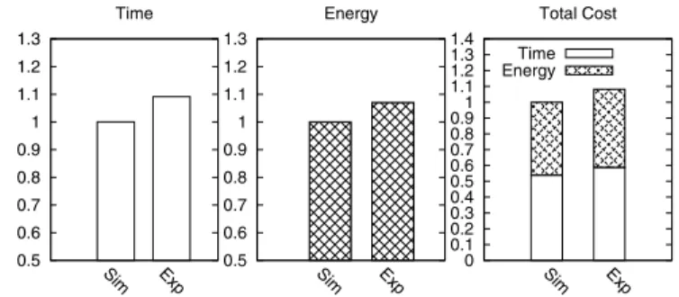
collect the time and energy data with a power meter. Then, we convert the collected data into the cost and compare it with the simulation result. Figure 1 shows the comparison results. The actual cost of executing the workloads on the x86 machine is about 8% higher than the simulation result. The main reason is that even if workloads are running simultaneously on different cores, they can still affect each other, e.g., by competing for last-level cache or memory. Such resource contention may cause longer execution times, and result in higher energy consumption and overall cost. We deem the 8% discrepancy acceptable because considering all the system-level overheads would make the scheduling problem too complicated to analyze.
0.5 0.6 0.7 0.8 0.9 1 1.1 1.2 1.3 Sim Exp Normalized Cost (%) Time 0.5 0.6 0.7 0.8 0.9 1 1.1 1.2 1.3 Sim Exp Energy 0 0.1 0.2 0.3 0.4 0.5 0.6 0.7 0.8 0.9 1 1.1 1.2 1.3 1.4 Sim Exp Total Cost Time Energy
Figure 1. COMPARISON OF THE SIMULATION AND EXPERIMENT
RESULTS
3) Comparison with Other Scheduling Methods: We con-ducted experiments to compare the cost of our schedul-ing scheme with that of Opportunistic Load Balancing (OLB) [11] and Power Saving. OLB schedules a task on the core with the earliest ready-to-execute time. The main objective of OLB is to ensure the cores are fully utilized and finish the tasks in the shortest possible time. Power Saving, which restricts the frequency of a core to conserve energy, is widely used in the power-saving mode of mobile devices. For dynamic frequency scaling, we set the Linux frequency governor to “On-demand” for both OLB and Power Saving. If a core’s loading is higher than 85%, the frequency governor increases the core’s frequency to the largest available selection.
First, we generate the scheduling plans with Workload Based Greedy, Opportunistic Load Balancing, and Power Saving. Then, we execute the plans on the experimental platform and measure their costs. In this experiment, we limit the available frequencies inPower Savingto the lower half of the CPU frequency range, i.e., 1.6, 2.0, and 2.4 GHz. As in the previous section, we set Re at 0.1 cent per joule andRt at 0.4 cents per second.
Figure 2 shows the cost of the three scheduling plans. Workload Based Greedy consumes 46% less energy than Opportunistic Load Balancing with only a 4% slowdown in the execution time. The total cost reduction is about 27%. Compared withPower Saving,Workload Based Greedy
consumes 27% less energy and improves the execution time by 13%. 0.5 0.6 0.7 0.8 0.9 1 1.1 1.2 WBG OLB PS Normalized Cost (%) Time 0.5 0.6 0.7 0.8 0.9 1 1.1 1.2 1.3 1.4 1.5 1.6 1.7 1.8 1.9 WBG OLB PS Energy 0 0.1 0.2 0.3 0.4 0.5 0.6 0.7 0.8 0.9 1 1.1 1.2 1.3 1.4 1.5 1.6 1.7 WBG OLB PS Total Cost Time Energy
Figure 2. COST COMPARISON OF DIFFERENT SCHEDULING
METHODS
B. Experiment Results for the Online Mode
We conduct a trace-based simulation to verify the accu-racy of theLeast Marginal Costalgorithm. The experimental environment is the same as that in Section V-A. The work-load is a piece of the trace from Judgegirl [12], which is an online judging system in National Taiwan University. The length of the trace is half hours during the final exam. We treat the score querying requests from students asinteractive tasks, and the codes they submit as non-interactivetasks. There are 768 non-interactivetasks and 50525 interactive tasks in the trace.
We compare the cost of the following scheduling strate-gies: Opportunistic Load Balancing,On-demand, andLeast Marginal Cost. Opportunistic Load Balancing(OLB) [11] schedules a task on the core with the earliest ready-to-execute time. The objective of OLB is to ensure the cores are fully utilized and finish the tasks in the shortest possible time. OLB keeps the processing frequency of each core at the highest level.On-demand[13] is a strategy in Linux that decides the processing frequency according to the current core loading. Once a core’s loading reaches a predefined threshold, On-demandscales to the highest processing fre-quency of that core. On the other hand, if the loading is lower than threshold,On-demandreduces the processing frequency by one level. Since On-demand does not schedule tasks to core, we assign the arriving tasks to core in a round-robin fashion. Least Marginal Cost is the strategies we propose.
Re and Rt are set to 0.4 cents per joule and 0.1 cent per
second, respectively.
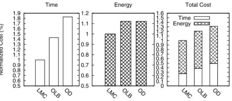
Figure 3 shows the cost comparison among scheduling methods.Least Marginal Cost method consumes 11% less energy and spends 31% less time thanOpportunistic Load Balancing, and has 17% less total cost. Similarly, Least Marginal Cost method consumes 11% less energy, spends 46% less time than the On-demand method, and has 24% less total cost. The results indicate thatLeast Marginal Cost heuristic saves energy and reduces task waiting time than existing algorithms.
0.5 0.6 0.7 0.8 0.9 1 1.1 1.2 1.3 1.4 1.5 1.6 1.7 1.8 1.9 LMC OLB OD Normalized Cost (%) Time 0.5 0.6 0.7 0.8 0.9 1 1.1 1.2 LMC OLB OD Energy 0 0.1 0.2 0.3 0.4 0.5 0.6 0.7 0.8 0.9 1 1.1 1.2 1.3 1.4 1.5 1.6 LMC OLB OD Total Cost Time Energy
Figure 3. COST COMPARISON OF DIFFERENT SCHEDULING
METHODS
VI. RELATEDWORK
Dynamic Voltage and Frequency Scaling (DVFS) is a key technique that reduces a CPU’s power consumption. There have been several studies of using DVFS, especially for applications in real-time system domains. The objective is to ensure that such applications can be executed in real-time systems without violating their deadline requirements, while minimizing the energy consumption. Yao et al. [4] proposed an offline optimal algorithm as well as an online algorithm with a competitive ratio for aperiodic real-time applications. Pillai et al. [14] presented a class of novel real-time DVS (RT-DVS) algorithms, including Cycle-conserving RT-DVS and Look-Ahead RT-DVS. Aydin et al. [5] developed an effi-cient solution for periodic real-time tasks with (potentially) different power consumption characteristics. However, the above works only consider single-core real-time systems, so they do not deal with the assignment of tasks to cores.
A number of recent studies of DVFS scheduling in real-time systems focused on multi-core processors. Kim et al. [3] proposed a dynamic scheduling method that incor-porates a DVFS scheme for a hard real-time heterogeneous multi-core environment. The objective is to complete as many tasks as possible while using the energy efficiently. Yang et al. [15] designed a 2.371 approximation algorithm that reduces the amount of energy used to process a set of real-time tasks that have common arrival times and deadlines on a chip multi-processor. Lee [16] introduced an energy-efficient heuristic that schedules real-time tasks on a lightly loaded multi-core platform. The above works focus on real-time systems in which tasks behave in a periodic or aperiodic manner. By contrast, the tasks considered in this paper are general computation tasks with or without deadlines.
In addition to real-time systems, some studies have inves-tigated using DVFS for other purposes. To minimize energy consumption, Bansal et al. [17] performed a comprehensive analysis and proposed an online algorithm to determine the processing speed of tasks with deadlines on a processor that has arbitrary speeds. Pruhs et al. [18] investigated a problem setting where a fixed energy volume E is given and the goal is to minimize the total flow time of the tasks.
They considered the offline scenario where all the tasks are known in advance and showed that optimal schedules can be computed in polynomial time. Albers et al. [9] developed an approach that uses a weighted combination of the energy and flow time costs as the objective function and exploits dynamic programming to minimize it in an offline fashion. This is similar to our approach, except that Albers et al. consider unit-size tasks, whereas our tasks can be any arbitrary size. Lam et al. [10] also studied scheduling to minimize the flow time and energy usage in a dynamic speed scaling model. They devised new speed scaling functions that depend on the number of active jobs, and proposed an online scheduling algorithm for batched jobs based on the new functions. The above works focus on single processors with discrete speeds. However, we consider both single and multi-core architectures in a per-core DVFS fashion.
Other energy-efficient algorithms have been proposed for multi-core platforms. Bunde [19] investigated flow time minimization in multi-processor environments with a fixed amount of energy. Aupy et al. [20] performed a com-prehensive analysis of executing a task graph on a set of processors. The goal is to minimize the energy consumption while enforcing a prescribed bound on the execution time. They considered different task graphs and energy models. In contrast to our approach, their method assumes that the mapping of tasks to cores is given, which is different to our approach.
VII. CONCLUSION
In this paper, we propose effective energy-efficient scheduling algorithms for multi-core systems with DVFS features. We consider two task execution modes: thebatch mode for batches of jobs; and the online mode for a more general execution scenario whereinteractivetasks with different time constraints or deadlines and non-interactive tasks may co-exist in the system. For each execution model, we propose scheduling algorithms and prove that they are effective both analytically and empirically. The algorithms solve three problems simultaneously: the assignment of tasks to CPU cores, the execution order of tasks, and the CPU core frequency for executing each task.
For thebatchmode, we prove that (1) the decision about the processing ratepk used to minimize the cost C(k, pk)
only depends onk, the position of the task in the execution sequence for a CPU core; and (2) the decision is independent of the execution workload of the task. We also show that there exists a polynomial-time optimal solution with the minimum cost in which the tasks are assigned in a greedy fashion in non-decreasing order of the number of cycles to the cores. Based on our theoretical findings, we propose a scheduling algorithm calledWorkload Based Greedy. For the onlinemode, we propose a heuristic calledLeast Marginal Cost, which assignsinteractiveandnon-interactivetasks to cores. It also determines the processing speeds that will
minimize the total cost of every time interval during a task’s execution.
Our experiment results show that, for the batch mode, the Workload Based Greedy algorithm consumes 46% less energy than the Opportunistic Load Balancing algorithm, with only a 4% slowdown in the execution time. It also achieves a 27% improvement in energy consumption and a 13% improvement in the execution time over the widely used Power Savingmethod. For theonlinemode, theLeast Marginal Cost algorithm yields a 17% and 24% improve-ment in the total cost compared with two existing algorithms in a trace-based simulation.
ACKNOWLEDGMENT
This work is supported by Information and Communica-tions Research Laboratories, Industrial Technology Research Institute, project number D352B83220.
REFERENCES
[1] P. Grosse, Y. Durand, and P. Feautrier, “Methods for power optimization in soc-based data flow systems,” ACM Trans. Des. Autom. Electron. Syst., vol. 14, no. 3, pp. 38:1–38:20, Jun. 2009.
[2] S. Lee and T. Sakurai, “Run-time voltage hopping for low-power real-time systems,” in Proceedings of the 37th Annual Design Automation Conference, ser. DAC ’00. New York, NY, USA: ACM, 2000, pp. 806–809.
[3] S. I. Kim, H. T. Kim, G. S. Kang, and J.-K. Kim, “Using dvfs and task scheduling algorithms for a hard real-time heterogeneous multicore processor environment,” in Proceedings of the 2013 Workshop on Energy Efficient High Performance Parallel and Distributed Computing, ser. EEHPDC ’13. New York, NY, USA: ACM, 2013, pp. 23–30.
[4] F. Yao, A. Demers, and S. Shenker, “A scheduling model for reduced cpu energy,” inProceedings of the 36th Annual Symposium on Foundations of Computer Science, ser. FOCS ’95. Washington, DC, USA: IEEE Computer Society, 1995, pp. 374–.
[5] H. Aydin, R. Melhem, D. Moss´e, and P. Mej´ıa-Alvarez, “Determining optimal processor speeds for periodic real-time tasks with different power characteristics,” in Proceedings of the 13th Euromicro Conference on Real-Time Systems, ser. ECRTS ’01. Washington, DC, USA: IEEE Computer Society, 2001, pp. 225–.
[6] K. Choi, K. Dantu, W.-C. Cheng, and M. Pedram, “Frame-based dynamic voltage and frequency scaling for a mpeg decoder,” in Proceedings of the 2002 IEEE/ACM International Conference on Computer-aided Design, ser. ICCAD ’02. New York, NY, USA: ACM, 2002, pp. 732–737.
[7] Y.-M. Chang, P.-C. Hsiu, Y.-H. Chang, and C.-W. Chang, “A resource-driven dvfs scheme for smart handheld devices,”
ACM Trans. Embed. Comput. Syst., vol. 13, no. 3, pp. 53:1–53:22, Dec. 2013.
[8] J.-J. Chen, “Multiprocessor energy-efficient scheduling for real-time tasks with different power characteristics,” in
Proceedings of the 2005 International Conference on Parallel Processing, ser. ICPP ’05. Washington, DC, USA: IEEE Computer Society, 2005, pp. 13–20.
[9] S. Albers and H. Fujiwara, “Energy-efficient algorithms for flow time minimization,” ACM Trans. Algorithms, vol. 3, no. 4, Nov. 2007.
[10] T.-W. Lam, L.-K. Lee, I. K. To, and P. W. Wong, “Speed scaling functions for flow time scheduling based on active job count,” in Proceedings of the 16th Annual European Symposium on Algorithms, ser. ESA ’08. Berlin, Heidelberg: Springer-Verlag, 2008, pp. 647–659.
[11] T. D. Braun, H. J. Siegel, N. Beck, L. L. B¨ol¨oni, M. Maheswaran, A. I. Reuther, J. P. Robertson, M. D. Theys, B. Yao, D. Hensgen, and R. F. Freund, “A comparison of eleven static heuristics for mapping a class of independent tasks onto heterogeneous distributed computing systems,” J. Parallel Distrib. Comput., vol. 61, no. 6, pp. 810–837, Jun. 2001.
[12] “Judgegirl,” https://github.com/ntuparallellab/judgegirl. [13] V. Pallipadi and A. Starikovskiy, “The ondemand governor:
past, present and future,” inProceedings of Linux Symposium, vol. 2, pp. 223-238, 2006.
[14] P. Pillai and K. G. Shin, “Real-time dynamic voltage scaling for low-power embedded operating systems,” inProceedings of the eighteenth ACM symposium on Operating systems principles, ser. SOSP ’01. New York, NY, USA: ACM, 2001, pp. 89–102.
[15] C.-Y. Yang, J.-J. Chen, and T.-W. Kuo, “An approximation algorithm for energy-efficient scheduling on a chip multi-processor,” inDesign, Automation and Test in Europe, 2005. Proceedings, 2005, pp. 468–473 Vol. 1.
[16] W. Y. Lee, “Energy-saving dvfs scheduling of multiple peri-odic real-time tasks on multi-core processors,” inDistributed Simulation and Real Time Applications, 2009. DS-RT ’09. 13th IEEE/ACM International Symposium on, 2009, pp. 216– 223.
[17] N. Bansal, T. Kimbrel, and K. Pruhs, “Speed scaling to manage energy and temperature,”J. ACM, vol. 54, no. 1, pp. 3:1–3:39, Mar. 2007.
[18] S. Irani and K. R. Pruhs, “Algorithmic problems in power management,”SIGACT News, vol. 36, no. 2, pp. 63–76, Jun. 2005.
[19] D. P. Bunde, “Power-aware scheduling for makespan and flow,” in Proceedings of the Eighteenth Annual ACM Symposium on Parallelism in Algorithms and Architectures, ser. SPAA ’06. New York, NY, USA: ACM, 2006, pp. 190–196.
[20] G. Aupy, A. Benoit, F. Dufoss´e, and Y. Robert, “Reclaiming the energy of a schedule: models and algorithms,” Concur-rency and Computation: Practice and Experience, vol. 25, no. 11, pp. 1505–1523, 2013.