Central Washington University
ScholarWorks@CWU
All Master's Theses Master's Theses
Spring 2018
DECREASING OCCLUSION AND
INCREASING EXPLANATION IN
INTERACTIVE VISUAL KNOWLEDGE
DISCOVERY
Abdulrahman Ahmed Gharawi
Central Washington University, [email protected]
Follow this and additional works at:https://digitalcommons.cwu.edu/etd
Part of theArtificial Intelligence and Robotics Commons, and theGraphics and Human Computer Interfaces Commons
This Thesis is brought to you for free and open access by the Master's Theses at ScholarWorks@CWU. It has been accepted for inclusion in All Master's
Recommended Citation
Gharawi, Abdulrahman Ahmed, "DECREASING OCCLUSION AND INCREASING EXPLANATION IN INTERACTIVE VISUAL KNOWLEDGE DISCOVERY" (2018).All Master's Theses. 941.
DECREASING OCCLUSION AND INCREASING EXPLANATION IN INTERACTIVE VISUAL KNOWLEDGE DISCOVERY
__________________________________
A Thesis Presented to The Graduate Faculty Central Washington University
___________________________________
In Partial Fulfillment
of the Requirements for the Degree Master of Science
Computational Science
___________________________________
by
Abdulrahman Ahmed Gharawi May 2018
CENTRAL WASHINGTON UNIVERSITY Graduate Studies
We hereby approve the thesis of
Abdulrahman Ahmed Gharawi Candidate for the degree of Master of Science
APPROVED FOR THE GRADUATE FACULTY
______________ _________________________________________
Dr. Boris Kovalerchuk, Committee Chair
______________ _________________________________________
Dr. Razvan Andonie
______________ _________________________________________
Dr. Szilard Vajda
______________ _________________________________________
ABSTRACT
DECREASING OCCLUSION AND INCREASING EXPLANATION IN INTERACTIVE VISUAL KNOWLEDGE DISCOVERY
by
Abdulrahman Ahmed Gharawi May 2018
Lack of explanation and occlusion are the major problems for interactive visual knowledge discovery, machine learning and data mining in multidimensional data. This thesis proposes a hybrid method that combines visual and analytical means to deal with these problems. This method, denoted as FSP, uses visualization of n-D data in 2-D in a set of Shifted Paired Coordinates (SPC). SPC for n-D data consists of n/2 pairs of Cartesian coordinates that are shifted relative to each other to avoid their overlap. Each n-D point is represented as a directed graph in SPC. It is shown that the FSP method simplifies pattern discovery in n-D data providing explainable rules in a visual form with significantly decrease of the cognitive load for analysis of n-D data. The computational experiments on real data has shown its efficiency on both training and validation data.
ACKNOWLEDGEMENTS
Firstly, I would like to express my sincere gratitude to my advisor Profs. Boris Kovalerchuk for his continuous support and endless advice, for his patience, motivation, and immense knowledge. His patient guidance, encouragement, and advice helped me all during the time of my research and master's study.
Besides my advisor, I would like to thank the rest of my thesis committee: Profs. Razvan Andonie and Szilárd Vajda, for their insightful comments, endless advice, and encouragement.
My sincere thanks also goes to professor Donald Davendra who provided me with unfailing support and continuous encouragement throughout my years of study.
Last but not least, I would like to thank my family: my parents, my wife Jumana Alsubhi, and my daughter, for supporting me spiritually throughout writing this thesis and my life in general.
TABLE OF CONTENTS
Chapter Page
I INTRODUCTION ... 1
SHIFTED PAIRED COORDINATES ... 2
II VISUAL KNOWLEDGE DISCOVERY ... 5
FSP ALGORITHM ... 5
FREQUENCY VISUALIZATION ALGORITHM ... 10
III EXPERIMENTAL CASE STUDIES ... 12
EXPERIMENTAL CASE STUDY 1 ... 12
EXPERIMENTAL CASE STUDY 2 ... 18
EXPERIMENTAL CASE STUDY 3 ... 23
EXPERIMENTAL CASE STUDY 4 ... 27
IV CONCLUSION ... 31
COMPARISON WITH PUBLISHED RESULTS ... 31
CONCLUSION ... 32
REFERENCES ... 34
APPENDIXES ... 36
Appendix A—WISCONSIN BREAST CANCER (WBC) ... 36
Appendix B—IONOSPHERE DATASET ... 36
Appendix C—ABALONE DATASET ... 36
Appendix D—MNIST DATASET ... 37
LIST OF TABLES
Table Page
1 Number of cases that satisfy the if part of Rule 1 in 11 random 70%:30%
splits of data ... 12
2 Precision, recall and coverage of Rule 1 in 11 random 70%:30% splits of data ... 13
3 Parameters of rectangles R1-R3 ... 13
4 Confusion matrixes of WBC Rule 2 ... 16
5 Parameters of rectangles R4-R6 in normalized coordinates ... 17
6 Confusion matrix of combined rules 1 and 3 on all 688 cases ... 17
7 Number of cases that satisfy the Ionosphere Rule 1 in 11 random 70%:30% splits of data ... 19
8 Precision, recall and coverage of Ionosphere Rule 1 in 11 random 70%:30% splits of data ... 19
9 Parameters of rectangles R1-R10 in normalized coordinates ... 19
10 Confusion matrixes of the Ionosphere Rule 2. ... 21
11 Number of cases satisfying the if part of Abalone Rule 1 in 11 random 70%:30% splits. ... 25
12 Precision, recall and coverage of Rule 1 in 11 random 70%:30% splits of data ... 25
13 Parameters of rectangles R1-R11 ... 27
LIST OF FIGURES
Figure Page
1 6-D point a=(3,2,1,4,2,6) in Shifted Paired Coordinates ... 2
2 A set of 688 Wisconsin Breast Cancer (WBC) data visualized in SPC as 2-D graphs of 10-D points with benign cases in Red and malignant cases in Blue ... 3
3 Overall design of the FSP process. ... 9 4 Alternative frequency visualization ... 11
5 WBC data in SPC as graphs representing 10-D points that go through R1 without showing frequency of cases. Magenta boxes show rectangles
R1-R3 ... 14
6 WBC data in SPC as graphs representing 10-D points that satisfy Rule 1 (go through R1 and not coming to R2 and R3 shown in magenta.
Wide Redlines show the frequency of Red cases ... 14 7 Remaining WBC cases not covered by Rule (dominated by Blue class) ... 15
8 WBC data in 4-D SPC as graphs in coordinates (X9,X8) and (X6,X7) that
are used by Rule 1, i.e., WBC cases that go through R1 and not go to R2
and R3 in these coordinates ... 16
9 The precision, recall and total coverage of combined Rule 1 and Rule 3 .. 17 10 351 Ionosphere cases in the SPCs as graphs of 34-D points
(good cases in Red and bad cases in Blue). Rectangles that are used in Ionosphere Rule 1 are in magenta ... 21
11 34-D Ionosphere cases covered by Ionosphere Rule 1 Rectangles from Rule 1 are in magenta ... 21
12 Remaining Ionosphere cases (cases not covered by Ionosphere Rule 1) ... 22 13 Ionosphere cases in 20-D points covered by the Ionosphere Rule 1 ... 22
LIST OF FIGURES
Figure Page
14 Ionosphere cases in 20-D points covered by Rule 1 ... 23 15 Ionosphere cases in 20-D points not covered by Rule 1 ... 23 16 A set of 2870 Abalone data visualized in the SPCs, as graphs of 8-D
points, with the male cases in Red, and the infant cases in Blue. Rectangles used in Abalone Rule 1 are in magenta. ... 25 17 8-D Abalone cases covered by Abalone Rule 1 ... 26 18 8-D Abalone cases covered by Rule 1 ... 26
19 Remaining Abalone cases (cases not covered by Abalone Rule 1) show the frequency of Red cases ... 27
20 Sum and average digits 0 and 1 in gray scale ... 29 21 SPC pairs presented as black dots in 22x22 empty image for 1 and 0 ... 29 22 SPC pairs presented as dark dots in the average of sum image
of 1 and 0 ... 30
23 SPC pairs presented as dark dots in the average of sum image of 1 and 0 magenta ... 30
CHAPTER I INTRODUCTION
For a long time, lack of explanation and occlusion have been the major problems for interactive visual knowledge discovery, data mining and machine learning in multidimensional data. This thesis proposes a hybrid method that combines visual and analytical means to deal with these problems in visual knowledge discovery. The proposed method, denoted as FSP, uses visualization of n-D data in 2-D in a type of General Line Coordinates (GLC) [Kovalerchuk, Grishin, 2017, Kovalerchuk, 2018] known as Shifted Paired Coordinates (SPC). A set of Shifted Paired Coordinates for n-D data consists of n/2 pairs of Cartesian coordinates that are shifted relative to each other without overlap. Each n-D point A is represented as a directed graph A* in SPC, where each node of the graph is a 2-D projection of A in a respective pair of the Cartesian coordinates.
The proposed FSP method significantly decreases cognitive load for analysis of n-D data and simplifies discovery of explainable patterns in n-D data. At the upper level, the steps of the FSP are: (1) Filtering out less efficient visualizations from multiple SPC visualizations, (2) Searching for sequences of paired coordinates that are more efficient, and (3) Presenting the SPC visualizations only with better sequences to the analyst. FSP includes the randomized search for pairs of coordinates and explainable “rectangular” classification rules with maximized
accuracy on training and validation data.
The computational experiments with the 9-D Wisconsin Breast Cancer data, 33-D
Ionosphere data, and 8-D Abalone data from UCI Machine Learning repository show efficiency of the FSP method on training and validation data. The visualization process in SPC is
n-D case. This hybrid visual analytics method allows classifying data in a way that can be communicated to the domain experts such as medical doctors in the explainable/understandable and visual form.
Shifted Paired Coordinates: Challenge and Opportunity to Better Visualization
The Shifted Paired Coordinates (SPC) visualization of n-D data requires splitting n coordinates X1-Xn to pairs producing n/2 non-overlapping pairs (Xi,Xj), such as (X1,X2), (X3,X4),
(X5,X6),…,(Xn-1,Xn) [Kovalerchuk, 2014; Kovalerchuk, Grishin, 2017, Kovalerchuk, 2018]. In
SPC, each pair (Xi,Xj) is represented as a separate orthogonal Cartesian Coordinates (X,Y),
where Xi is X and Xj is Y.
In SPC visualization design each coordinate pair (Xi,Xj) is shifted relative to other pairs to
avoid their overlap. This creates n/2 scatter plots. Next in SPC, for each n-D point
x=(x1,x2,…,xn), the point (x1,x2) in (X1,X2) is connected to the point (x3,x4) in (X3,X4) and so on
until point (xn-2,xn-1) in (Xn-2,Xn-1) is connected to the point (xn-1,xn) in (Xn-1,Xn) to form a
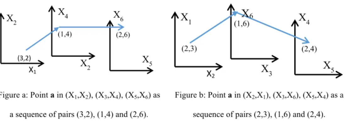
directed graph x*. Figure 1 shows the same data visualized in SPC in two different ways due to different pairing of coordinates.
Figure a: Point a in (X1,X2), (X3,X4), (X5,X6) as
a sequence of pairs (3,2), (1,4) and (2,6).
Figure b: Point a in (X2,X1), (X3,X6), (X5,X4) as a
sequence of pairs (2,3), (1,6) and (2,4). Figure 1: 6-D point a=(3,2,1,4,2,6) in Shifted Paired Coordinates.
X1 X2 X2 X4 X5 X6 (3,2) (1,4) (2,6) X2 X1 X3 X5 X4 (2,3) (1,6) (2,4) X6
In general, there are multiple combinatorial ways to form pairs of coordinates for SPC and to sequence pairs. The SPC visualization graphs xk* of each given n-D point x differ for different
sequences Sk of pairs of coordinates. Fig. 1a illustrates it for a 6-D point a=(3,2,1,4,2,6)
visualized in pairs (X1,X2), (X3,X4), (X5,X6), and Fig. 1b shows this point visualized in pairs
(X2,X1), (X3,X6), (X5,X4).
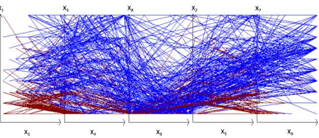
The SPC allows visualizing each individual n-D point losslessly, but together graphs of multiple n-D points occlude each other. See Fig. 2. This creates a difficulty for discovering patterns to classify cases of opposing classes in SPC. In Fig. 2 some areas are visibly dominated by cases of the specific color. However, it is not sufficient to build discrimination rules to
classify cases visually. It required an addition analytical process. Such process is proposed in this thesis. SPC visualizations with some sequences Sk can reveal classification patterns of n-D data
better than with using other sequences. The dependence of the visualization from the different pairing coordinates creates a challenge and an opportunity to find better pairs and their
sequences.
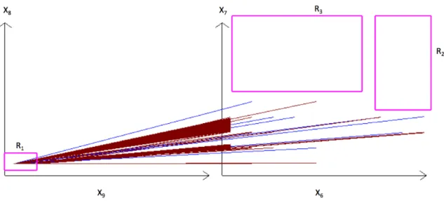
Figure 2: A set of 688 Wisconsin Breast Cancer (WBC) data visualized in SPC as 2-D graphs of 10-D points with benign cases in Red and malignant cases in Blue.
The challenge is that it is impractical to conduct interactive search of efficient sequences of pairs of coordinates for the large number of sequences. The total number of pairs of n
coordinates is the number of combinations C(n,2)=n!/((n-2)!×2!), e.g., 45 for n=10. Next, there are multiple different sequences of the same set of n/2 pairs, e.g., (X1,X2),(X3,X4),(X5,X6),…,(X n-1,Xn) and (X5,X6),(X3,X4),(X1,X2),…,(Xn-1,Xn).The number of these sequences (orders) is (n/2)!
for the same set of n/2 pairs, e.g., (10/2)!=120 for n=10. Thus, the total number of sequences of all pairs of n coordinates is (n/2)!×C(n,2)= (n/2)!×n!/((n-2)!×2!) and for n=10 it is 45×120=5400. The analyst cannot observe all of them to find one with the best visual separation of classes. The FSP algorithm resolves this issue by automatic search for the best sequences and presenting only a few best visualizations to the analyst.
CHAPTER II
VISUAL KNOWLEDGE DISCOVERY
FSP Algorithm
The FSP algorithm:
(a) Filters out less efficient rules and visualizations for supervised classification learning, (b) Searches for sequences of pairs of coordinates and respective rules that are more efficient
for supervised classification learning, and
(c) Presents the SPC visualizations only with better sequences to the analyst.
The main characteristic of FSP is avoiding interactive exploration of the exponential number of alternative sequences with the following major steps:
Step 1: Random generation of sequences of pairs of coordinates S; Step 2: SPC representation of n-D data in sequences S from Step 1;
Step 3: Machine learning process for learning “rectangular” classification rules with high accuracy, precision and recall in sequences S from Step 2;
Step 4: Full automated visualization process: SPC representation of best n-D rules in the best full sequences S of pairs of coordinates S discovered in Step 3;
Step 5: Simplified automated visualization process: SPC representation of best n-D rules in the best subsequences S of pairs of coordinates S discovered in Step 3;
Step 6: Interactive visualization process: an analyst interactively controls and manages produced SPC visualizations.
The approach of this algorithm is in line with [Wilinski, Kovalerchuk, 2017]. It produces efficient classification rules and 3-D visualization of n-D data. In that paper another visualization
method called Collocated Tripled Coordinates from the class of General Line Coordinates (GLC) is combined with Machine Learning for predicting the investment strategy.
The ideas of steps 1 and 2 already have been explained above. The step 3 uses rules and learning criteria presented below.
Rules and Learning Criteria. The filtering works on a set of rules such as rules (RL1)-(RL8) listed below. Each Rule is defined on an n-D point x=(x1,x2,…,xn) to be classified to some
classes:
If (xi,xj) Î R1 then xÎ class 1, (RL1)
If (xi,xj) Î R1 & (xk,xm) Î R2 & (xs,xt) Î R3 then xÎ class 1 (RL2)
If ((xi,xj) Î R1 Ú (xk,xm) Î R2 ) & (xs,xt) Î R3 then xÎ class 1 (RL3)
If ((xi,xj) Î R1 Ú (xk,xm) Î R2 ) & (xs,xt) Ï R3 then xÎ class 1 (RL4)
If ((xi,xj) Î R1 Ú (xk,xm) Î R2 ) & (xs,xt) Ï R3 then xÎ class 1, else xÎ class 2 (RL5)
If (xi,xj) Î R1 & (xk,xm) Î R2 & (xs,xt) Ï R3 then xÎ class 1 (RL6)
If (xi,xj) Î R1 & (xi,xj) Ï R2 & (xi,xj) Ï R3 then xÎ class 1 (RL7)
If (xi,xj) Î R1 Ú (xk,xm) Ï R2 v (xs,xt) Ï R3 then ) xÎ class 1 (RL8)
where R1, R2 and R3 are specific rectangles, in respective pairs of Cartesian coordinates in a
given sequence S of pairs of coordinates S, e.g., R1 can be in (X1,X2).
The filtering follows common Data Mining/Machine Learning strategy of learning rules on training data and validation on validation data. The quality of learning of classification and expected visualization for rules (RL1)-(RL4), (RL6)-(RL8) is measured by the precision and
recall of classification of training and validation data, where the precision Pr is the fraction of the of cases predicted correctly by the Rule to the all predicted cases by the Rule:
Pr= |{cases predicted correctly by the Rule}| / |{all predicted cases by the Rule}|.
The precision Pr for the basic Rule (RL1): If (xi,xj) Î R1 then x Î class 1, is calculated as
follows:
𝑃𝑟 = $%('()
$%('()*$+('() (9) where n1(R1) is the number of points of class 1 in R1 (i.e., the number of correctly classified
cases), and n2(R1) is the number of points from class 2 in R1 (i.e., the number of misclassified
cases). More generally, for any Rule(x) such that
If Rule(x) then xÎ class 1 (10) the precision is
𝑃𝑟 =$%(,-./)*$+(,-./)$%(,-./) (11) where n1(Rule) is the number of points of class 1 that satisfy the if part of the Rule and n2(Rule) is the number of points of class 2 that satisfy the if the part of the Rule too.
The formula (11) is applicable to all rules (RL1)-(RL8). For example, the precision Pr for the Rule (RL4) is calculated as follows:
𝑃𝑟 = $%('()*$%('0)1$%('(&'3)1$%('0&'3)
$%('()*$%('0)1$%('(&'3)1$%'0&'3)*$+('()*$+('0)1$+('(&'3)1$+('0&'3) (12) where
n1(R1) and n1(R2) are the number of points of class 1 in R1, R2, respectively,
n2(R1&R3) is the number of graphs x* of the n-D points of class 2 that have 2-D points in both R1 and R3, nb(R2&R3) is the number of graphs x* of the n-D points of class 2 that have 2-D points in both R2 and R3. Here
𝑛1(𝑅%) + 𝑛1(𝑅+) − 𝑛1(𝑅%&𝑅9) − 𝑛1(𝑅+&𝑅9) is the number of correctly classified n-D points by Rule
(RL4) and 𝑛2(𝑅%) + 𝑛2(𝑅+) − 𝑛2(𝑅%&𝑅9) − 𝑛2(𝑅+&𝑅9) is the number of misclassified n-D points by
this Rule.
We use precision for rules (RL1)-(RL4) and (RL6)-(RL8) instead of accuracy because these rules predict only one class. All cases that do not satisfy the condition of these rules are not classified (refused to be classified). The computing accuracy would require predictions of the class for all cases as it is the case for rules (RL5). Therefore, rules in set of rules (RL5) we use the accuracy for filtering. Note that a high precision Rule from sets of rules (RL1)-(RL4), (RL6)-(RL8) may covers only a few cases, but the precision value does not show it’s low coverage. Therefore, we also use the recall
RC = |{cases predicted correctly by the Rule}| / |{all cases}| that is a fraction of cases correctly predicted by the Rule to all cases to be predicted.
The Random generation in Step 1 consists of two substeps:
(RS1) Randomly generate a set of pairs of coordinates from coordinates X1-Xn,
(RS2) Randomly generate sequence Sk for a set of pairs from (RS1).
The Machine Learning process in Step 3 consists of following three substeps:
(ML1) Search for rectangles in each (Xi,Xj) that maximize precision or accuracy of a
Rule from (RL1)-(RL8) on training data for given Sk,
(ML2) Evaluate this Rule on validation data,
(ML3) Combine promising rules to get a stronger Rule in precision, accuracy and recall. The Automated Visualizationprocess in Steps 4-5 consists of the following steps:
(AV1) Visualize in SPC most accurate classification results. This includes visualization of only best results.
(AV2) Remove data that are covered by best results in (IV1),
(AV3) Repeat (RS1-RS2) and (ML1-ML3) for remaining data in search for the best classification results.
The Interactive Visualizationprocess in Step 6 is as follows:
(IV1) Substitute automatic search in (ML1) by interactive search where the analysts select rectangles in SPC visualization using GUI.
(IV2) The automatic system supports this interactive process by computing accuracies of rules based on selected rectangles and removing data covered by best results found before the next interactive selection of new rectangles starts.
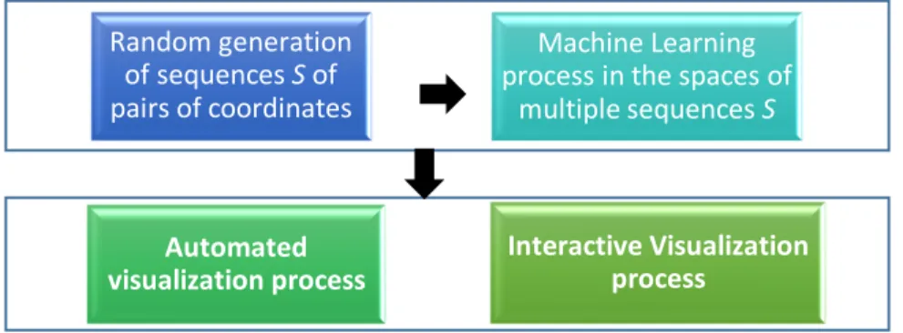
Fig. 3 shows the overall design of the FSP process.
Figure 3: Overall design of the FSP process.
Random generation of sequences Sof pairs of coordinates
Machine Learning process in the spaces of
multiple sequences S
Automated
Frequency Visualization Algorithm
One of the challenges of SPC visualization for larger data sets is a form of occlusion caused by a limited resolution of data on the screen. It leads to overlap of similar data including complete colocation of some lines. In addition, identical cases will collocate on any visualization at any resolution. Therefore, the task is enhancing the SPC visualization to show frequency of the lines.
The algorithm for this, denoted as FRE algorithm, consists of the following steps:
(F1) For each consecutive pairs of coordinates (Xi,Xj), (Xk, Xm) form sets of edges {Eq} that are
collocated or nearly collocated under some threshold T, (F2) Count the number of edges Cq(T) in each of these sets,
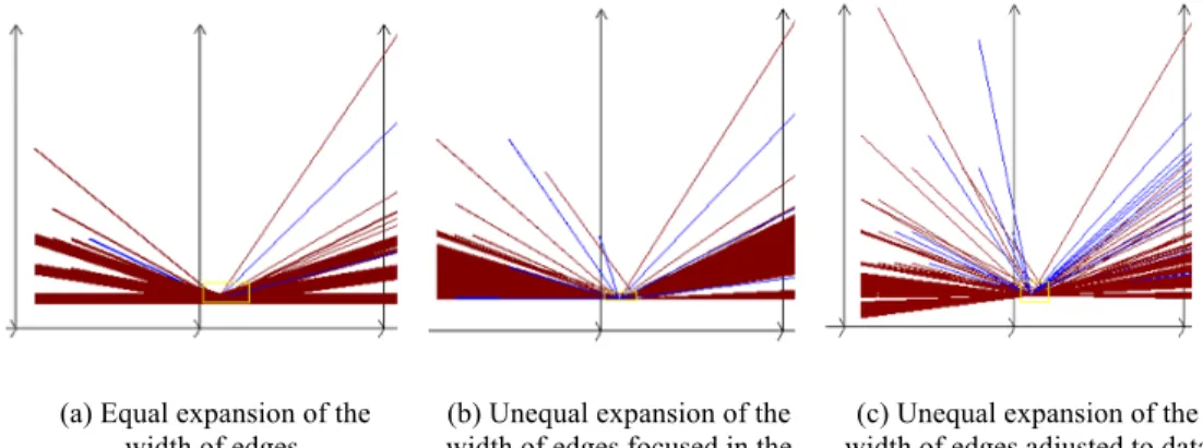
(F3) Draw each such set of edges Eq with the adjustable width w:
(a) Equally proportional to the number of edges in Eq for each node,
(b) Unequally proportional to the number of edges in Eq for each node without adjusting to
the data density,
(c) Unequally proportional to the number of edges in Eq for each node with adjusting to the
data density.
Fig. 4 illustrates the differences between versions (a)-(c) of the algorithm FRE for Red graphs in SPC. The version (a) is “neutral”, the analyst can use it when no specific node it set up to explore, Versions (b) and (c) are for exploring specific nodes of interest (e.g. nodes of the discovered classification Rule), because the large width of edge in (a) may occlude that specific node.
(a) Equal expansion of the
width of edges. width of edges focused in the (b) Unequal expansion of the given node of graph.
(c) Unequal expansion of the width of edges adjusted to data
density focused in the given node of graph.
CHAPTER III
EXPERIMENTAL CASE STUDIES
Experimental Case Study 1
The computational experiments with the 9-D Wisconsin Breast Cancer (WBC) data, from the UCI Machine Learning repository [3] presented below, show the efficiency of the FSP algorithm. To get the even number of coordinates and 5 pairs of coordinates, the coordinate X5
was duplicated in X10 getting total 10 coordinates.
The discovered patterns were found by the search in the set of rules (RL1)-(RL8). In particular, on WBC data, the FSP algorithm found an efficient sequence of the pairs of the coordinates. This sequence of pairs is (X5,X1), (X4,X3), (X9,X8), (X5, X2), (X6, X7). Here X5 is
used in two pairs (X5,X1) and (X5, X2). The SPC visualization with this sequence reveals
classification pattern with precision over 90% in all 11 random 70%:30% splits that are presented in Tables 1 and 2. The best precision on the training data is 99.3%, which is accompanied by the high precisions on the validation data (98.21%), in one of the 70%:30% splits of the given data into the training and the validation data.
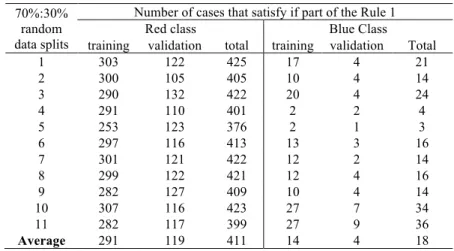
Table 1. Number of cases that satisfy the if part of Rule 1 in 11 random 70%:30% splits of data.
70%:30% random data splits
Number of cases that satisfy if part of the Rule 1
Red class Blue Class
training validation total training validation Total
1 303 122 425 17 4 21 2 300 105 405 10 4 14 3 290 132 422 20 4 24 4 291 110 401 2 2 4 5 253 123 376 2 1 3 6 297 116 413 13 3 16 7 301 121 422 12 2 14 8 299 122 421 12 4 16 9 282 127 409 10 4 14 10 307 116 423 27 7 34 11 282 117 399 27 9 36
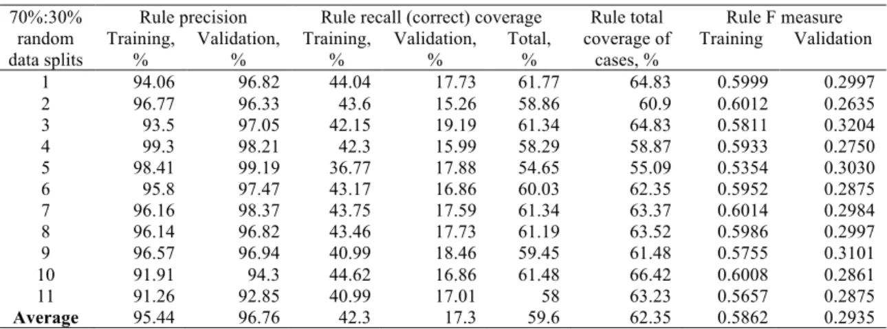
Table 2. Precision, recall and coverage of Rule 1 in 11 random 70%:30% splits of data. 70%:30%
random data splits
Rule precision Rule recall (correct) coverage Rule total coverage of
cases, %
Rule F measure Training,
% Validation, % Training, % Validation, % Total, % Training Validation 1 94.06 96.82 44.04 17.73 61.77 64.83 0.5999 0.2997 2 96.77 96.33 43.6 15.26 58.86 60.9 0.6012 0.2635 3 93.5 97.05 42.15 19.19 61.34 64.83 0.5811 0.3204 4 99.3 98.21 42.3 15.99 58.29 58.87 0.5933 0.2750 5 98.41 99.19 36.77 17.88 54.65 55.09 0.5354 0.3030 6 95.8 97.47 43.17 16.86 60.03 62.35 0.5952 0.2875 7 96.16 98.37 43.75 17.59 61.34 63.37 0.6014 0.2984 8 96.14 96.82 43.46 17.73 61.19 63.52 0.5986 0.2997 9 96.57 96.94 40.99 18.46 59.45 61.48 0.5755 0.3101 10 91.91 94.3 44.62 16.86 61.48 66.42 0.6008 0.2861 11 91.26 92.85 40.99 17.01 58 63.23 0.5657 0.2875 Average 95.44 96.76 42.3 17.3 59.6 62.35 0.5862 0.2935
The discovered rules in Tables 1 and 2 belong to the set of rules (RL7). The first Rule in Table 1 that we denote as WBCRule 1 is:
If (x9,x8) Î R1 & (x6,x7) ÏR2 & (x6,x7) ÏR3 then xÎ class 1 (Red, Benign) (13)
where R1,R2,and R3 are specific rectangles, in respective pairs of Cartesian coordinates (X8,X9)
and (X6, X7). Table 3 shows the parameters of R1,R2 and R3 in the normalized coordinates. Table 3. Parameters of rectangles R1-R3.
Rectangle Parameters
Left Right Bottom Top
R1 in (X9,X8) 0.0020 0.1402 0.0734 0.1028
R2 in(X6,X7) 0.7214 1.001 0.3484 1.001
R3 in (X6,X7) 0.0081 0.6325 0.6014 1.001
This Rule, with a random 70%:30% data split into the training and the validation data, has the precision of 94.6% on the training data, and 96.82% on the validation data. Figs. 5 and 6 show its rectangles R1, R2 and R3 drawn in the SPC as magenta boxes. The difference between
these figures is that Fig. 5 shows all graphs that go through rectangle R1 (have node (x9,x8) in R1),
but Fig. 6 shows only graphs that in addition do not go rectangles R2 and R3.(do not have node
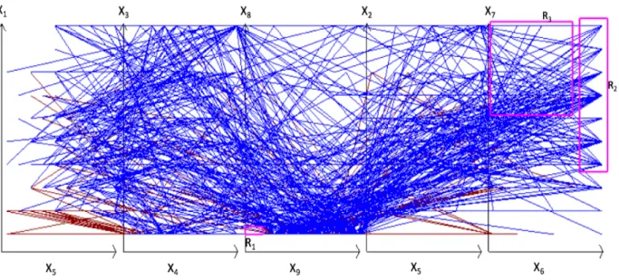
Figure 5: WBC data in SPC as graphs representing 10-D points that go through R1 without showing frequency of cases. Magenta boxes show rectangles R1-R3.
In Fig. 5, the width of the lines are not adjusted their frequency, but in Fig. 6 the width of the lines is adjusted to their frequencies. The Rule 1 covers 64.8% of all given 9-D points: 446 cases out of 688 cases (425 Red cases and 21 Blue cases) with the recall value 61.77% (425/688) as shown in Table 1. Among these 446 cases 303 Red and 17 Blue cases belong to training data and 122 Red and 4 Blue cases belong to validation data.
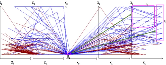
Figure 6: WBC data in SPC as graphs representing 10-D points that satisfy Rule 1 (go through R1 and not coming to R2 and R3 shown in magenta. Wide Red lines show the frequency of Red cases.
The cases covered by Rule 1 do not include only the 5.13% (23 cases) of the Red data, but include the 91.25 % (219 cases) of the Blue data. This Rule covers only cases found in R
that do not come to R2 or R3. Rule 1 refused to predict other cases. Those other cases are
dominantly Blues (see Fig. 7) and must be covered by other rules. The WBC Rule 1 uses only 4 coordinates that form two pairs (X9,X8) and (X6,X7) therefore we can simplify the visualization
of this Rule by showing only them in SPC. It is done in Fig. 8 where each 4-D points is
visualized losslessly as a single line. The advantage of this visualization is that it is easy to see and communicate to the medical experts. The medical expert can easily understand this Rule because it simply says that two attributes x8 and x9 must be in some limits identified in Table 3
and two other attributes x6 and x7 must not have values in some intervals that are shown visually
in Fig. 8.
This allows the medical experts to analyze the consistency of this Rule with the other medical domain knowledge, which is extremely difficult for the ML discrimination functions, which are “black” boxes or complex mathematical formulas.
Figure 8: WBC data in 4-D SPC as graphs in coordinates (X9,X8) and (X6,X7) that are used by Rule 1, i.e., WBC cases that go
through R1 and not go to R2 and R3 in these coordinates.
The simple WBCRule 2 classifies all remaining cases (not covered by Rule 1) to class 2 is If (x8,x9) Î R1 & (x6,x7) ÏR2 & (x6,x7) ÏR3
then xÎ class 1 (Red, Benign) else xÎ class 2 (Blue, Malignant) (14) This Rule classifies all cases that are either in R2 or in R3 or not in R1 as Blue. This Rule has
accuracy 93.60% (425+219)/688) on all 688 cases as the confusion matrix shows in Table 4. Its accuracy on training data is 92.53% and on validation data it is 96.11% computed from
respective confusion matrixes shown in Table 4.
Table 4. Confusion matrixes of WBC Rule 2. Actual class Confusion matrix on all 688 cases Confusion matrix on 70% of training cases (482) Confusion matrix on 30% on validation cases (206) Predicted class Predicted class Predicted class
Red Blue Total Red Blue Total Red Blue Total
Red 425 23 448 303 19 322 122 4 126
We found a better WBCRule 3 by searching the rectangles with highest density of Blue cases: If ((x1,x6) Î R4Ú (x3,x5) Î R5) & (x2,x5) Ï R6 then xÎ class 2 ( Blue ) (15)
This Rule is of type of rules (RL4), but with the conclusion that x belongs to class 2, not class 1. Table 5 identifies the rectangles R4-R6 involved in this Rule. WBC Rule 3 covers the 226 cases
from class 2 (Blue), and the 12 cases from class 1 (Red) with the total precision of 94.95%. The
combined Rule1 and Rule 3 is as follows:
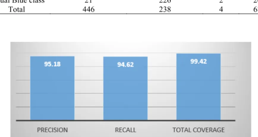
If Rule1(x) then xÎRed, else if Rule3(x) then xÎBlue, else refuse to classify x (16) The precision, recall and coverage of this Rule relative to all cases are 95.18%, 94.62%, and
99.42% (Fig. 9). It is the performance details are in the confusion matrix in Table 6.
Table 5. Parameters of rectangles R4-R6 in normalized coordinates.
Rectangle Parameters
Left Right Bottom Top
R4 in (X1,X6) 0.0010 0.9712 0.4180 1.001
R5 in (X3,X5) 0.0000 0.9881 0.3154 0.7261
R6 in (X2,X5) 0.0000 0.1003 0.143 0.3153
Table 6. Confusion matrix of combined Rules 1 and 3 on all 688 cases. Predicted Red class Predicted Blue class Refusal Total
Actual Red class 425 12 2 437
Actual Blue class 21 226 2 247
Experimental Case Study 2
The computational experiments with the 33-D Ionosphere data from the UCI Machine Learning repository [3] also show the efficiency of the FSP algorithm. To get the even number of coordinates and 17 pairs of coordinates, the algorithm in each epoch will select randomly the coordinate that will serve as coordinate X34. In the following results X34 is a copy of X10. The
discovered patterns also were found by the search in the set of “rectangular” rules (RL1)-(RL8). In particular, on Ionosphere data, the FSP algorithm found an efficient sequence of pairs of coordinates: (X5, X26), (X27, X16), (X4, X11), (X18, X24), (X28, X31), (X10,X3), (X23, X8), (X22, X30),
(X21, X10), (X17, ), (X15,X33), (X29, X20), (X9, X6), (X32,X16), (X1,X25), (X12, X14), (X19, X7). Here
X10 is repeated in pairs (X10, X3) and (X21, X10). Similarly to the Case Study 1, the SPC
visualization, with this sequence, reveals the visual classification pattern of precision of over 90% in all the 11 random 70%:30% splits of data into the training and the validation data (see Tables 7 and 8). The best precision on the training data is 98.36% with 100% precision on the validation data in one of these 70%:30% splits of the given data. The discovered rules in Tables 7 and 8 belong to the set of rules (RL4). The first Rule in Table 7 that we denote as Ionosphere Rule 1 is:
If [(x4,x11) Î R1Ú (x5,x26) Î R8 Ú (x21,x10) Î R9Ú (x19,x7) Î R10] &
[(x27,x16)Ï R3 & (x28,x31) ÏR6 & (x23,x8)ÏR4 & (x17,x2) Ï R5 & (x15,x33)Ï R7 & (x9,x6)Ï R2]
then x Î class 1 (Red ,Good) (17) where R1, R2, R3, R4, R5, R6, R7, R8, R9, and R10 are specific rectangles, in respective pairs of
Cartesian coordinates (X4, X11), (X9, X6), (X27, X16), (X23, X8), (X17, X2), (X28, X31), (X15, X33),
has the precision 98.36% on the training data and 100% on validation data. Figs. 10 and 11 show its rectangles R1-R10 in the SPCs as magenta boxes and cases that satisfy Rule 1 in Fig 11 and all
cases in Fig. 10. Fig. 12 shows the remaining cases.
Table 7. Number of cases that satisfy the Ionosphere Rule 1 in 11 random 70%:30% splits of data.
70%:30% random data splits
Number of cases that satisfy if part of the Rule 1
Red class Blue Class
training validation total training validation Total
1 180 45 225 3 0 3 2 172 52 224 8 2 10 3 133 92 225 7 3 10 4 129 95 224 6 2 8 5 200 24 224 9 0 3 6 160 65 225 10 2 12 7 183 42 225 11 1 13 8 158 67 225 11 2 13 9 191 34 225 13 1 14 10 184 37 221 7 0 7 11 157 66 223 12 2 14 Average 170 54 224 9 1 9
Table 8. Precision, recall and coverage of Ionosphere Rule 1 in 11 random 70%:30% splits of data. 70%:30%
random data splits
Rule precision Rule recall (correct) coverage Rule total coverage of
cases, %
Rule F measure Training,
% Validation, % Training, % Validation, % Total, % Validation, % Total, %
1 98.36 100 51.28 12.82 64.1 64.95 0.6741 0.2273 2 95.55 96.29 49 14.81 63.81 66.6 0.6478 0.2567 3 95 96.84 37.89 26.21 64 66.95 0.5417 0.4125 4 95.5 97.93 36.75 27.06 63.81 66.09 0.5308 0.4240 5 95.69 100 56.98 6.83 63.81 64.67 0.7143 0.1279 6 94.1 97.01 45.58 18.51 64.1 67.52 0.6141 0.3109 7 94.32 97.67 52.13 11.96 64.1 67.80 0.6715 0.2131 8 93.491 97.1 45.01 19.08 64.09 67.80 0.6077 0.3189 9 93.62 97.14 54.41 9.68 64.1 68.09 0.6882 0.1761 10 96.33 100 52.421 10.54 62.96 64.95 0.6789 0.1907 11 92.89 97.05 44.72 18.8 63.53 67.52 0.6037 0.3150 Average 94.99 97.93 48.43 15.38 63.81 66.38 0.6339 0.2703 Table 9. Parameters of rectangles R4-R6 in normalized coordinates.
Rectangle Parameters
Left Right Bottom Top
R1 in (X4, X11) 0.23912 1.001 0.663667 0.999667 R2 in(X9, X6) 0.1979 0.99869 0 0.0403333 R3 in(X27, X16) 0.130225 1.001 0 0.0256667 R4 in(X23, X8) 0.29087 0.58943 1.001 0.946 R5 in(X17, X2) 0.40433 0.9998 0 0.022 R6 in(X28, X31) 0.30765 1.001 0 0.0366667 R7 in(X15, X33) 0.25733 1.001 0.960667 0.998667 (X, X ) 0.125675 0.575667 0.575667 0.645333
The Rule 1 uses only 20 coordinates that form 10 pairs (X5 ,X26),(X27 ,X16), (X4,X11),
(X28,X31), (X23,X8),(X21,X10),(X17,X2),(X15,X33),(X9 ,X6) and (X19 ,X7). Therefore, we simplify
its visualization by showing only them in the SPCs (see Figs. 13-15) with the lossless
visualization of each of the 20-D points, as a single polyline. The simple IonosphereRule 2
classifies all remaining cases (not covered by Rule 1) to class 2 is If [(x4,x11) Î R1Ú (x5,x26) Î R8 Ú (x21,x10) Î R9Ú (x19,x7) Î R10] &
[(x27,x16)Ï R3 & (x28,x31) ÏR6 & (x23,x8)ÏR4 & (x17,x2) Ï R5 & (x15,x33)Ï R7 & (x9,x6)ÏR2]
then x Î class 1 (Red, Good) else x Î class 2 (Blue, Bad) (18) This Rule classifies all the cases rejected by Rule 1 as Blue with 99.14% accuracy on all the 351 cases (225+123)/351), see the confusion matrix in Table 10. Its accuracy on training data is 98.78% and 100% on the validation data based on the confusion matrixes in Table 10.
Figure 10: 351 Ionosphere cases in the SPCs as graphs of 34-D points (good cases in Red and bad cases in Blue). Rectangles that are used in Ionosphere Rule 1 are in magenta.
Figure 11: 34-D Ionosphere cases covered by Ionosphere Rule 1. Rectangles from Rule 1 are in magenta.
Table 10. Confusion matrixes of the Ionosphere Rule 2. Actual
class Confusion matrix on all 351 cases Confusion matrix on training data (246, 70%) Confusion matrix on validation data (206, 30%) Predicted class Predicted class Predicted class
Red Blue Total Red Blue Total Red Blue Total
Red 225 3 228 180 3 183 45 0 45
Blue 0 123 123 0 63 63 0 60 60
Figure 12: Remaining Ionosphere cases (cases not covered by Ionosphere Rule 1).
Figure 14: Ionosphere cases in 20-D points covered by Rule 1.
Figure 15: Ionosphere cases in 20-D points not covered by Rule 1.
Experimental Case Study 3
The computational experiments with the 8-D Abalone data, male and infant cases, from the UCI Machine Learning repository [3] also show the efficiency of the FSP algorithm. The
particular, the FSP algorithm found an efficient sequence of coordinate pairs: (X5, X6), (X1, X2),
(X3, X8), (X4, X7). Similarly, to Case Studies 1 and 2, the SPC visualization, with this sequence,
reveals the visual classification pattern of with the precision of over 90% (see Tables 11 and 12) in the 11 random 70%:30% splits of data into the training and the validation cases. The best precision is 92.06% on the training data and 96.17% on the validation data. Fig. 16 shows 2870 Abalone data in the SPCs, as graphs of 8-D points, with the male cases in Red, and the infant cases in Blue. Rectangles used in Abalone Rule 1 defined below are in magenta. Fig.17 and 18 show cases covered this Rule and Fig. 19 shows the remaining cases.
The discovered rules shown in the Tables 11 and 12 belong to the set of rules (RL4). The first Rule in the Table 11, which we denote as the AbaloneRule 1 is:
If [(x4,x7) Î R1Ú (x1,x2) Î (R2Ú R8)Ú (x3,x8) Î(R4 Ú R6) ] & [(x5,x6) Ï ( R3 & R10 & R11 )
& (x1,x2) Ï(R5& R9) & (x3,x8) Ï(R4 & R7)], then xÎ class 1 (Red ,Male), (19)
where R1, R2, R3, R4, R5, R6, R7, R8, R9, R10, and R11 are specific rectangles (see Table 13), in
respective pairs of the Cartesian coordinates (X4, X7), (X1, X2), (X5, X6), (X3, X8), (X1, X2), (X3,
X8), (X3, X8), (X1, X2), (X1, X2), (X5, X6), and (X5, X6). The simple Abalone Rule 2, which
classifies all the remaining cases (not covered by Rule 1) into class 2 is:
If [(x4,x7) Î R1Ú (x1,x2) Î (R2Ú R8)Ú (x3,x8) Î(R4 Ú R6) ] & [(x5,x6) Ï ( R3 & R10 & R11 )
&(x1,x2) Ï(R5& R9) & (x3,x8) Ï(R4 & R7) ]
then xÎ class 1 (Red, Male), else xÎ class 2 (Blue, Infant) (20) with accuracy 94.91% on all cases, 93.33% and 98.60% on training and validation data based on the confusion matrixes Table 14.
(a) Red cases visualized on the top Blue cases. (b) Blue cases visualized on the top the Red cases.
Figure 16: A set of 2870 Abalone data visualized in the SPCs, as graphs of 8-D points, with the male cases in Red, and the infant cases in Blue. Rectangles used in Abalone Rule 1 are in magenta.
Table 11. Number of cases satisfying the if part of Abalone Rule 1 in 11 random 70%:30% splits. 70%:30%
random data splits
Number of cases that satisfy if part of the Rule 1
Red class Blue Class
training validation total training validation Total
1 1193 304 1497 103 12 115 2 1034 396 1430 103 37 140 3 972 463 1435 86 46 132 4 1015 484 1499 105 40 145 5 1224 272 1496 126 10 136 6 1003 371 1374 98 28 126 7 989 402 1391 92 37 129 8 1077 389 1466 108 22 130 9 1146 328 1474 117 31 148 10 1201 276 1477 121 15 136 11 996 357 1353 103 35 138 Average 1078 367 1445 106 29 134
Table 12. Precision, recall and coverage of Rule 1 in 11 random 70%:30% splits of data. 70%:30%
random data splits
Rule precision Rule recall (correct) coverage Rule total coverage of cases, % Rule F measure Training, % Validation, % Training, % Validation, % Total, % Validation, % Total, % 1 92.05 96.20 41.56 10.59 52.16 56.16 0.5727 0.1908 2 90.94 91.45 36.02 13.79 49.82 54.70 0.5160 0.2397 3 91.87 90.96 33.86 16.13 50 54.59 0.4948 0.2740 4 90.62 92.36 35.36 16.86 52.22 57.28 0.5087 0.2851 5 90.66 96.45 42.64 9.47 52.12 56.86 0.5800 0.1725 6 91.09 92.98 34.94 12.92 47.87 52.26 0.5051 0.2269 7 91.48 91.57 34.45 14.00 48.46 52.96 0.5005 0.2429 8 90.88 94.64 37.52 13.55 51.08 55.6 0.5311 0.2371 9 90.73 91.36 39.93 11.42 51.35 56.51 0.5545 0.2030 10 90.84 94.84 41.84 9.616 51.46 56.2 0.5729 0.1746 11 90.62 91.07 34.70 12.43 47.14 51.95 0.5018 0.2187 Average 91.07 93.06 37.53 12.80 50.33 55.01 0.5307 0.2241
(a) Red cases on the top of the Blue cases. (b) Blue cases on the top of the Red cases. (a) F u l l g r a p h s . (b) O n l y n o d e s o f g r a p h s Figure 17: 8-D Abalone cases covered by Abalone Rule 1.
Figure 19 : Remaining Abalone cases (cases not covered by Abalone Rule 1).
Table 13. Parameters of rectangles R1-R11.
Rectangle Parameters
Left Right Bottom Top
R1 in (X4, X7) 0.09068 0.6946 0.260333 1.00 R2 in(X1, X2) 0.7458 0.99955 0.421667 0.99996 R3 in(X5, X6) 0.0209 0.1015 0.128333 0.190667 R4 in(X3, X8) 0.94857 1.001 0 0.077 R5 in(X1, X2) 0.162175 0.253525 0.242 0.113667 R6 in(X3, X8) 0.46645 0.77602 0.139333 0.399667 R7 in(X3, X8) 0.25837 0.38017 0.282333 0.388667 R8 in(X1, X2) 0.355025 0.415925 0.355667 0.436333 R9 in(X1, X2) 0.26 0.355025 0.161333 0.242 R10 in(X5, X6) 0.015075 0.167325 0.289667 0.436333 R11 in(X5, X6) 0.012 0.035675 0.0 0.0586667
Table 14. Confusion matrixes of Abalone Rule 2. Actual
class Confusion matrix on all 2870 cases Confusion matrix on trai-ning cases (2009, 70%) Confusion matrix on validation cases (861, 30%) Predicted class Predicted class Predicted class
Red Blue Total Red Blue Total Red Blue Total Red 1497 115 1612 1193 103 1296 304 12 316 Blue 31 1227 1258 31 682 713 0 545 545 Total 1528 1342 2870 1224 785 2009 304 557 861
Experimental Case Study 4
These computational experiments conducted with digits 0 and 1 represented as the 484-D points (cases) show the efficiency of the FSP algorithm. The discovered patterns were found by the search in the set of “rectangular” rules (RL1)-(RL8). The training data contain 703 0 and 778 1. The discovered Rule1 has a form of a Rule 4 (see page 11). It contains 132 rectangles that are spread around 78 242 paired coordinates with average of 1.69 rectangles per pair. In contrast with case studies 1-3, in this case study we did not conduct pair permutation and used the original order of pairs: (X1,X2), (X3,X4),…,(Xn-1,Xn) due to multiplicity of pairs.
This multiplicity also creates a challenge to visualize all 484 dimensions in SPC that are used by FSP algorithm. This reveals one of the limitations of FSP algorithm based on SPC for the direct visualization of discrimination rules. Therefore, below we propose a generalized visualization of a discrimination rules for such high-dimensional data (images). The idea of a new visualization is to “overlay” the discrimination Rule1 on the input images of digits.
The steps of the new algorithm that we denote as R2I (Rectangles In Image) below:
(a) Compute the average image M(0) for digit 0 by averaging all respective pixels of the training data of this digit:
M(0)={m(i,j): m(i,j)=averagekÎK(Tr(0,k,i,j)}
where K is the number of digits 0 in the training data and Tr(0,k,i,j) is the intensity of the pixel (i,j) of the k-th image of digit 0. See figure 20.
(c) Compute the average image T for digit 0 and 1 by averaging M(0) and M(1). figure 22. (d) Find location of the pairs of pixels in the image 21 for digit 0 that have been used in
rectangles in the discovered Rule1. For instance, let pixels 71 and 72 form a pair of coordinates (X71,X72) and the rectangle R1 from Rule1 is discovered in these coordinates.
(e) Show pixels 71 and 72 in black. Do this for all rectangles involved in the Rule 1. The result is in figure 21 and figure 22.
(f) Conduct steps (d)-(e) for digit 1. The result is in Figure 21 and figure 22.
Figure 21: SPC pairs presented as black dots in 22x22 empty image for 1 and 0.
The result has a precision over 90% in random 70%:30% splits of data into the training and the validation date. The best precision obtained is 96.21% on the training data and 98.03% on the validation data. Fig. 21 represents the SPC pairs locations as a dark dot in an empty 22x22 image. Fig. 22 shows 2115 MINST data in the average of sums for number 0 and 1 as an image of 22x22 pixels (484 dimensions). The dark dots represent pairs that been covered by the rules.
Figure 23: SPC pairs presented as dark dots in the average of sum image of 1 and 0. Figure 22: SPC pairs presented as dark dots in the average of sum image of 1 and 0.
CHAPTER IV CONCLUSION
Comparison with Published Results
Case study 1: the best accuracy reported for the Wisconsin Breast Cancer (WBC) dataset for the SVM in [6] is 96.995% with the 10-fold cross-validation tests. Other results are 96.84% [7] and 96.99% [8] for the SVM, and 97.28% [6] by combing SVM, C4.5 decision tree, naïve Bayesian classifier, and the k-Nearest Neighbors algorithms.
These models classify all the cases, while many of our rules refuse to classify some of the cases. Our WBC Rule 2 classify all cases, but with lower accuracy 93.60%. Our better Rule that combines WBC rules 1 and 3 has precision 95.18%. While in general, accuracy and precision are different, here the combination of rules 1 and 3 cover almost all cases (99.42%, only 4 cases are refused). The precision for such high coverage is almost identical to accuracy. Thus, it is quite close to the published results, but slightly lower. However, in contrast with SVM, it is visual, has clear interpretation and explainable to a domain expert which is very important in domains with high cost of errors where the explanation of the model is mandatory.
Case study 2: for Ionosphere dataset, the highest accuracy reported by [9] is 98% on training and 93% on validation data using the multilayer perceptron. Other results are 94.87% by using C4.5 algorithm and 94.59% using Rule Induction RIAC algorithm [10], 97.33% by SVM with Particle Swarm Optimization and 10-fold cross-validation [11].
These models classify all the objects, while many of our rules refuse to classify some of the cases. In contrast, our Ionosphere Rule 2 classify all cases. For this Rule, precision is identical to accuracy that is 98.78% on training data and 100% on validation data. Thus, our results are
Case study 3: The highest accuracy reported in [12] for Abalone dataset using SVM is 99.26% with 5-fold Cross-validation for all three classes. Another result is 97.80% accuracy using a case base reasoning method [13]. Our result, that are within [93.33, 98.60]% interval, are quite close to these published results. Unlike [12], we use a more challenging approach for classification 70:30 split, than the 5-fold that is 80:20 split.
The goal of [15] was to find large empty rectangles or boxes in 1D, 2D, 3D, 4D, and 5D spaces. This goal differs from our goal of finding 2-D rectangles filled by points of a single class or dominated by that class. This we have a ‘reverse” task. Also, the focus of [15] is designing a new computationally efficient algorithm to find holes in high dimensional data that runs in polynomial time. This is different from FSP algorithm too. Unlike the empty rectangles in [15], FSP algorithm use the rectangles in 2D to classify data. Also, FSP try to find rectangle that contains the points that belong to specific class and reduce the error by finding another rectangle that classify the wrong cases in the first rectangle. The potential use in [15] for strengthening FSP using algorithm from [15] to search most non-empty rectangles in 2-D or remove most empty before searching for non-empty. For non-empty rectangles it is likely that algorithm from [15] must be modified.
Conclusion
The FSP Rule 2 for Wisconsin Breast Cancer (WBC), Ionosphere and Abalone are visual, interpretable, and explainable to a domain expert, which is critical, in many domains with
mandatory model explanation. This comparison shows that the proposed FSP algorithm, with the SPC visualization, produced the results comparable with the other major machine learning algorithms, in the accuracy and precision. The FSP algorithm has the following significant
advantages: it is (i) visual with minimal occlusion, (ii), interactive, (iii) understandable by the user, and (iv) simpler than many machine-learning algorithms.
Future study would focus on using more interpretable rules for discovery by the FSP algorithm along with the other General Line Coordinates, beyond SPC. Also, to optimize the search time, by discard the highly correlated coordinates in random generation of pairs. That reduces run time between 5 to 30 percent in some cases. Another way to optimize the search of rectangles is to use one of the evolutionary algorithms instead of purely random ones to find the best possible sequence and pairs. The directed search will increase the chance of reducing the time and improving the accuracy.
REFERENCES
1. Kovalerchuk B., Gharawi A., Decreasing Occlusion and Increasing Explanation in Interactive
Visual Knowledge Discovery, In: Human Interface and the Management of Information. Interaction, Visualization, and Analytics, Lecture Notes in Computer Science series, Vol. 10904, 2018, Springer
2. Kovalerchuk, B., Grishin, V. Adjustable general line coordinates for visual knowledge
discovery in n-D data. Inf. Vis. 2017, doi:10.1177/1473871617715860.
3. Kovalerchuk B. Visual Knowledge Discovery and Machine Learning, 2018, Springer. 4. Lichman, M. UCI Machine Learning Repository, http://archive.ics.uci.edu/ml, 2013. 5. Wilinski, A., Kovalerchuk, B. Visual knowledge discovery and machine learning for
investment strategy. Cognitive Systems Research, v. 44, 2017, pp. 100–114.
6. Salama, G.I.,Abdelhalim, M., Zeid, M.A. Breast cancer diagnosis on three different datasets
using multi-classifiers. Breast Cancer (WDBC) 2012, 32, 2.
7. Aruna, S., Rajagopalan, D.S., Nandakishore, L.V. Knowledge based analysis of various
statistical tools in detecting breast cancer. Comput. Sci. Inf. Technol. 2011, 2, 37–45.
8. Christobel, A., Sivaprakasam, Y. An empirical comparison of data mining classification
methods. Int. J. Comput. Inf. Syst. 2011, 3, 24–28.
9. Duch W,Kordos M.Multilayer perceptron with numerical gradient.ICANN2003,106-109. 10.Hamilton HJ, Shan N., Cercone N., RIAC: a Rule induction algorithm based on approximate
classification. Computer Science Department, University of Regina; 1996.
11.Tu, C.-J., Chuang, L, Y., Yang, C.H. Feature selection Using PSO-SVM. IAENG Int. J.
classification. Procedia Computer Science. 2015,1;72:59-66.
13.Smiti A., Elouedi Z. Maintaining Case Based Reasoning Systems Based on Soft Competence
Model. In Intern. Confer. on Hybrid Artificial Intelligence Systems 2014,666-677. Springer.
14.Y. LeCun and C. Cortes, “MNIST handwritten digit database,
APPENDIXS APPENDIX A
WISCONSIN BREAST CANCER (WBC)
Wisconsin Breast Cancer (WBC) dataset from the UCI machine learning repository [3]. WBC dataset contains 699 instances with 11 attributes. The patient ID was removed from the first dimension. Also, each instance that contains a missing value was removed in the preprocessing phase. That produces 688 records with 448 of benign and 240 with malignant cases. In addition, the dataset was normalized between 0 and 1.
APPENDIX B
IONOSPHERE DATASET
Ionosphere dataset is from the UCI machine learning repository [3]. This dataset contains 351 instances with 35 attributes where 35th dimension represents the class label of good cases and bad cases. In the preprocessing step, the second dimension was removed because it only contains zeros resulting 34-D. Also, the dataset was rescaled between 0 and 1.
APPENDIX C
ABALONE DATASET
Abalone dataset is a dataset from the UCI machine learning repository [3]. This dataset contains 4177 instances with eight attributes for predicting the age of Abalone from physical measurements [3]. The 8th attribute represents the classes label. In the preprocessing step, cases of the female were removed resulting 1612 male and 1258 infant cases.
APPENDIX D
MNIST-DATASET
In order to test the FSP method on high dimensional data, the Modified National Institute of Standards and Technology (MNIST) [14] was used. MNIST Database originally consists of images for digits from 0 to 9 with 28x28 pixels (784 dimensions) for each image. The digits 0 and 1 in the validation dataset was used after removing the padding. The preprocessed images contain a total of 2115, 1135 images of digit 1 and 981 of digit 0 with 22x22 pixels (484 dimensions) each.