Statistical Methods for Analyzing Bivariate Mixed Outcomes

(1)

Doctoral Dissertations University of Connecticut Graduate School

9-11-2017

Statistical Methods for Analyzing Bivariate Mixed

Outcomes

Ved Deshpande

University of Connecticut - Storrs, [email protected]

Follow this and additional works at:https://opencommons.uconn.edu/dissertations

Recommended Citation

Deshpande, Ved, "Statistical Methods for Analyzing Bivariate Mixed Outcomes" (2017).Doctoral Dissertations. 1615.

(2)

Mixed Outcomes

Ved Deshpande, Ph.D. University of Connecticut, 2017

ABSTRACT

Multivariate outcomes are ubiquitous. Joint analysis of multivariate outcomes provides several benfits over separate analysis of each outcome. However, joint analysis of mul-tivariate outcomes that are mixed, i.e., not on the same scale of measurement, can be challenging. This dissertation provides novel methods to analyze bivariate mixed outcomes, where we have exactly one continuous outcome and one binary outcome. A penalized generalized estimating equations framework to perform simultaneous esti-mation and variable selection for bivaraite mixed outcomes in the presence of a large number of covariates is provided. Next, fully Bayesian and empirical Bayes approaches to estimating the association between the two outcomes using a copula-based model are provided. Finally, methods for estimating and testing genomic effects in bivariate mixed secondary outcome models under case-control designs are presented.

(3)

Mixed Outcomes

Ved Deshpande

Integrated B.Sc. and M.Sc., Statistics and Informatics, Indian Institute of Technology, Kharagpur, India, 2010

A Dissertation

Submitted in Partial Fulfillment of the Requirements for the Degree of

Doctor of Philosophy at the

University of Connecticut 2017

(4)

Copyright by

Ved Deshpande

(5)

APPROVAL PAGE

Doctor of Philosophy Dissertation

Statistical Methods for Analyzing Bivariate Mixed

Outcomes

Presented by

Ved Deshpande, Integrated B.Sc. and M.Sc., Statistics and Informatics

Co-Major Advisor Dipak K. Dey Co-Major Advisor Elizabeth D. Schifano Associate Advisor Haim Bar University of Connecticut 2017

(6)

Acknowledgments

I would like to thank both of my advisors, Dr. Dipak Dey and Dr. Elizabeth Schifano, without whose support I could not have completed this dissertation. Dr. Dey gave me much advice on how to be a good researcher, and taught me how to “connect the dots” to develop new ideas. Dr. Schifano was with me in the trenches, providing me with unwavering support and encouragement, especially during those times when things seemed absolutely hopeless. From going line-by-line through proofs, to catching tiny bugs in my code that escaped me for weeks, to providing detailed corrections on manuscripts, Dr. Schifano has helped me at every step of the way. I would also like to thank her for giving me my first taste of research, by offering me a research assistantship during my second year.

I am also very grateful to Dr. Ming-Hui Chen, for selecting me to be a part of UCONN’s Statistical Consulting Services. Being a part of SCS has contributed tremen-dously towards my development as an applied statistician, and opened doors to a variety of career paths. I am certain that I would not have gotten the career opportunities that I have had without this experience. Dr. Chen has also been a role model of dedication and integrity. Seeing someone as incredibly busy as him never cut corners in even the smallest of tasks has inspired me to do the same, and I am better off for it.

(7)

committee, and for working with me on the research assistantship that I did in my second year. I learnt a great deal of R programming and applied statistics from him.

Next, I would like to thank every professor who has taught me at UCONN. They not only gave me an excellent education, but also infected me with their passion for statistics. In particular, I must thank Dr. Nitis Mukhopadhyay, who lit the first spark of my love for statistics; Dr. Rick Vitale, who showed me that measure theory was beautiful rather than terrifying; and Dr. Jun Yan, who helped me discover the power of the R programming language.

I have had a lot of fun during the last five years, and I owe that to no one more than my friends and colleagues in the department. Thank you for all the laughs, arguments, rants, philosophy, and motivation. I wish you all the best of luck in your endeavours.

Finally, and most importantly, I would like to thank my family for their constant support, warmth, and love. I dedicate this dissertation to you. Mom and Dad, you have always been supportive of my life choices, providing me with gentle guidance, and pulling me out of tight corners. Dooti, I have lost count of the innumerable number of things that you have done for me over these past eight years. Words utterly fail to capture my gratitude. Thank you–for everything.

(8)

List of Tables

1 Accuracy and variable selection metrics comparing the joint and the sep-arate PGEE methods, for θ = 0.2,0.4,0.6,0.8, with all covariates shared

between the continuous and binary outcomes. Maximum TP is 9.0 and maximum FP is 91. . . 29 2 Accuracy and variable selection metrics the comparing the joint and the

separate PGEE methods, for θ = 0.2,0.4,0.6,0.8, with some covariates shared between the continuous and the binary outcomes. Maximum TP is 9.0 and maximum FP is 91. . . 30 3 Accuracy and variable selection metrics comparing the joint and the

sep-arate PGEE methods, for θ = 0.2,0.4,0.6,0.8, with no covariates shared

between the continuous and the binary outcomes. Maximum TP is 9.0 and maximum FP is 91. . . 31 4 Absolute bias (AB) and sandwich-formula based standard errors (SE) of

estimates of true non-zero regression coefficients for the joint and the sep-arate PGEE methods, withall covariates shared between the continuous and binary outcomes. . . 33

(12)

5 Absolute bias (AB) and sandwich-formula based standard errors (SE) of estimates of true non-zero regression coefficients for the joint and the sepa-rate PGEE methods, withsome covariates shared between the continuous and the binary outcomes. . . 35 6 Absolute bias (AB) and sandwich-formula based standard errors (SE) of

estimates of true non-zero regression coefficients for the joint and the sep-arate PGEE methods, withno covariates shared between the continuous and the binary outcomes. . . 36 7 Covariates used in analysis of MEPS data . . . 41 8 Estimated regression coefficients for log(drug spending) and health

sta-tus outcomes under the joint and the separate PGEE methods. A dot indicates that the covariate was not selected by that method, for that outcome. Covariates that are not selected by either method are not shown. 42 9 Estimated regression coefficients and sandwich formula-based standard

errors for covariates selected by the joint method in the MEPS data anal-ysis. A dot in the Coefficient column indicates that the covariate was not selected for that outcome. . . 43 10 Bias, root mean square error, coverage of 95% credible intervals, and

average width of 95% credible intervals for model parameters, under the Fully Bayesian method (FB) and the empirical Bayes method (EB). . . . 66

(13)

11 Bias, root mean square error, coverage of 95% credible intervals, and average width of 95% credible intervals for the estimate of Kendall’s Tau

τ, under the Fully Bayesian method (FB) and the empirical Bayes method (EB). Data sets are generated with true τ ∈ {0.1,0.3,0.6}. . . 70 12 Average time differences in hours to complete parameter estimation

be-tween the fully Bayesian method (FB) and the empirical Bayes method (EB) ∆time. The difference in computation time for a single data set is computed as the time for EB minus the time for FB. . . 71 13 Fraction of 500 replications where a copula family used for estimation is

selected by the model selection metric, for varying values of Kendall’s Tau

τ, sample size n, and copula family used for data generation. The model selection metrics considered are the Deviance Information Criterion (DIC) and the Logarithm of Pseudo Marginal Likelihood (LPML). . . 73 14 DIC and LPML values for the models fitted on the burn injury data.

Models with smaller values of DIC and larger values of LPML are preferred. 76 15 Posterior means, standard deviations, and 95% credible intervals for the

parameters of the Gumbel copula model applied to the burn injury data. The top row shows the derived metrics for Kendall’s Tau τ. . . 77 16 Root mean square error (RMSE), bias, Type I error, and power for the

(14)

17 Type I error and power for the IPW method, for the separate tests H0 :

τc = 0 andH0 :τb = 0. . . 96

18 Top SNPs from the EAGLE study reaching genome-wide level of signifi-cance 5×10−8 for the testH :τc=τb = 0. The corresponding

Bonferroni-corrected p-values for the tests H:τc= 0 and H :τb = 0 are also shown.

Corrected p-values larger than 1 are truncated to 1 and marked with an asterisk (*). . . 98

(15)

List of Figures

1 Contour plots of smoothed true and estimated FDRs. The continuous penalty parameter is on the horizontal axis and the binary penalty pa-rameter is on the vertical axis. Each contour shows the combination of penalty parameters that result in the same true/estimated FDR. . . 37

(16)

Chapter 1

Introduction

The task of modeling multivariate outcomes on sets of covariates is becoming increasingly common across research disciplines. Multivariate outcomes that are measured from the same sampling unit are likely to be correlated. Joint modeling of correlated multivariate outcomes is preferable over separate modeling of the outcomes because we may be able to obtain more efficient parameter estimates through information sharing across correlated outcomes (Teixeira Pinto and Normand, 2009).

Multivariate outcomes are often mixed, i.e., they are measured on different scales of measurement. A common subcase of mixed multivariate outcomes is when exactly two outcomes per sampling unit are measured, with one outcome measured on a continuous scale and the other outcome measured on a binary scale. Joint modeling of suchbivariate mixed outcomes is usually performed by specifying a joint probability model for the outcomes. However, specifying a joint model for mixed outcomes is challenging due to the lack of appropriate multivariate distributions for mixed outcomes. Likelihood-based approaches that aim to circumvent this problem include the factorization approach, in which the joint distribution of the outcomes is factorized into the marginal distribution

(17)

of one outcome and the conditional distribution of the other outcome given the first outcome, and the latent variable approach, in which unobserved shared latent variables account for the correlation between the outcomes. See Teixeira Pinto and Normand (2009) for a survey of these methods. A drawback of the factorization approach is that the model is not invariant to the choice of the conditioning outcome (Wu and de Leon, 2014). Disadvantages of the latent variable approach include sensitivity to misspecification of the covariance structure, and arbitrary and untestable distributional assumptions on the latent variables (Prentice and Zhao, 1991).

To overcome the drawbacks of direct likelihood-based approached to model bivariate mixed outcomes, a few indirect approaches have been proposed. One class of approaches utilizes generalized estimating equations (GEEs) (Prentice and Zhao, 1991; Rochon, 1996; Liu et al., 2009). GEEs are both convenient and robust; convenient because GEEs only require the specification of the first two moments of each outcome and an approx-imation to their correlation structure, and robust because GEEs consistently estimate the regression parameters even if the correlation structure is misspecified. GEEs are primarily used when the correlation between the outcomes is a nuisance parameter, and the marginal parameters are of primary interest. On the other hand, in many research studies, the association between the outcomes is of primary interest. Because GEEs are inefficient for estimating association parameters (Liang et al., 1992; Hall and Severini, 1998), they are not appropriate in such cases. In this context, copulas (Nelsen, 2007) are a convenient tool to efficiently model the association between correlated outcomes.

(18)

Like GEEs, copulas do not require direct specification of a joint distribution between the outcomes. Rather, they “glue” the marginal distributions of the outcomes together. With the ability to specify marginal distributions independently and the vast number of dependence structures available (Joe, 2014), copulas provide researchers great flexibility in modeling correlated outcomes.

We now provide a brief introduction to the framework of GEEs and copulas. Note that for the latter, we consider two-dimensional copulas only, which are relevant to this dissertation.

1.1

Generalized estimating equations

Liang and Zeger (1986) introduced GEEs as an extension of generalized linear models (McCullagh, 1984) to account for the correlation between longitudinal outcomes. More generally, GEEs can be used with any kind of clustered outcomes, not necessarily lon-gitudinal. Suppose there are n clusters, and we observe outcomes yi = (yi1, . . . , yimi)

T_,

i = 1, . . . , n. Each outcome yij has associated with it a p-dimensional covariate vector xij, i = 1, . . . , n, j = 1, . . . , mi. Observations from different clusters are assumed to be

independent, but observations from the same cluster are assumed to be correlated. For notational simplicity, we assume that mi =m, i.e., all clusters are of the same size.

GEEs require specification of the first two moments of the outcomes. Similar to generalized linear models, we specify link functions gij(µij) =xTijβ, whereµij =E(yij).

(19)

Denote µi = (µi1, . . . , µim)T. Next, we specify variance functions vij(yij) = ψhij(µij).

Note that we have assumed that within a cluster, a common set of regression coefficients

β and a common dispersion parameter ψ apply to each outcome. This assumption will be relaxed in the chapters that follow. The GEEs are given by

S(β) = n−1 n X i=1 DT_iV_i−1(yi−µi) =0, whereDT

i =∂µi(β)/∂βT, andViis the variance-covariance matrix of yi, given byVi =

ψA1_i/2RA_i1/2, where Ai = diag(hi1(µi1), . . . , him(µim)), and R ≡((ρ_jj0)) is the working correlation matrix of (yi1, . . . , yimi)

T_{, assumed to be the same for all}_i_{= 1}_{, . . . , n}_{. Some}

commonly used working correlation structures include independence (ρ_jj0 = 0, j 6=j 0 ), exchangeable (ρ_jj0 =ρ, j 6=j 0 ), AR(1) (ρ_jj0 =ρ|j−j 0

|_{), and unstructured, among others.}

For simplicity, assume a single parameter ρ indexes R.

In practice, the GEEs are solved by iterating between a Newton-Raphson type update for β and moment-based estimation of (ψ, ρ)T. For more details on the moment-based estimators of ψ and ρ, see Liang and Zeger (1986). Given the current estimate βˆk _and

estimates ˆψ and ˆρ, the regression coefficients β are updated as

ˆ βk+1 =βˆk+ n X i=1 Di(βˆk)TV˜i −1 Di(βˆk) !−1" _n X i=1 Di(βˆk)TV˜i −1 ri(βˆk) # ,

(20)

solving the GEEs lead to consistent estimates of the regression parametersβ, even if the working correlation structure R is misspecified, which makes for convenient and robust inference.

1.2

Copulas

Sklar (1959) first introduced the termcopula in the statistical literature to denote tions that joined marginal distributions together to form a joint distribution. The func-tions themselves, however, can be traced back to Hoeffding (1940). Sklar’s theorem (Sklar, 1959) shows the relationship between the joint distribution function, the marginal distribution functions, and the copula.

Theorem 1.1 (Sklar’s Theorem). Let H be a joint distribution function of random variables Y1 and Y2 with margins F1 and F2. Then there exists a copula C such that

H(y1, y2) = C(F1(y1), F2(y2)), ∀(y1, y2)∈R2. (1.1)

If F1 and F2 are continuous, then C is unique. Otherwise, C is uniquely defined on

Range(F1) × Range(F2).

Conversely, if C is a copula and F1 andF2 are distribution functions, then the function

H defined by (1.1) is a joint distribution with margins F1 and F2.

(21)

F2 and C, the resulting H function is a valid joint probability distribution function. This allows for great flexibility in constructing joint probability distributions.

We have informally denoted copulas as functions that join marginal probability dis-tribution functions together to form a joint probability disdis-tribution. For the purposes of this dissertation, this is sufficient. Formal mathematical definitions of copulas can be found in Nelsen (2007).

1.2.1

Measures of dependence

With copulas, we can specify the type of dependence structure that we wish to model between random variables. Usually, parametric copula families are indexed by a param-eter θ, which controls the strength of dependence between the random variables. Two important measures of dependence are Kendall’s Tau and Spearman’s Rho, defined as follows:

Definition 1.2(Kendall’s Tau). For random variablesX1 andY1, the population version

of Kendall’s Tau is

τ =P[(X1−X2)(Y1−Y2)>0]−P[(X1−X2)(Y1−Y2)<0],

(22)

For continuous random variables X1 and Y1 with copula C, we have τ = 4 ˆ 1 0 ˆ 1 0 C(u1, u2)dC(u1, u2)−1. (1.2)

Definition 1.3 (Spearman’s Rho). For random variables X1 and Y1, the population

version of Spearman’s Rho is

ρ= 3(P[(X1−X2)(Y1−Y3)>0]−P[(X1 −X2)(Y1−Y3)<0],

where (X1, Y1), (X2, Y2), and (X3, Y3) are independent copies.

For continuous random variables X1 and Y1 with copula C, we have

ρ= 12 ˆ 1 0 ˆ 1 0 C(u1, u2)du1du2−3.

Another concept of dependence is tail dependence, which relates to the dependence between extreme values in the upper-right and the lower-left quadrant of a bivariate distribution.

(23)

margins F1 and F2 and copula C. Then define λL= lim u→0+P(Y2 ≤F −1 2 (u)|Y1 ≤F1−1(u)) = lim u→0+ C(u, u) u , λU = lim u→1−P(Y2 > F −1 2 (u)|Y1 > F1−1(u)) = 2− lim u→1− 1−C(u, u) 1−u .

C has lower tail dependence if λL ∈ (0,1], and lower tail independence if λL = 0, and similarly for upper tail dependence and λU.

1.2.2

Some commonly used copula families

Here we provide definitions and some useful properties of the copula families that are used in this dissertation. These copula families broadly belong to the elliptical and Archimedean classes of copulas. For details on these classes of copulas, see Nelsen (2007).

1. The Gaussian copula family belongs to the elliptical class of copulas. It is a symmetric copula that does not exhibit tail dependence. The two-dimensional Gaussian copula is given by

C(u1, u2|θ) = Φ2(Φ−1(u1),Φ−1(u2)|θ), θ∈(−1,1),

where Φ2(·,·|θ) is the bivariate standard normal distribution function with correlation parameter θ, and Φ−1 _{is the inverse of the univariate standard normal distribution}

(24)

function. For this copula, Kendall’s Tau is given byτ = (2/π)arcsinθ.

2. The Clayton copula family belongs to the Archimedean class of copulas. It is an asymmetric copula that exhibits lower tail dependence. The copula is given by

C(u1, u2|θ) = (u−1θ+u

−θ

2 −1)

1

θ, θ ∈(−1,∞)\ {0}.

For this copula, Kendall’s Tau is given by τ =θ/(θ+ 2).

3. The Gumbel copula family belongs to the Archimedean class of copulas. It is an asymmetric copula that exhibits upper tail dependence. The copula is given by

C(u1, u2|θ) = exp h − (−logu1)θ+ (−logu2)θ 1 θi_, _θ_∈_[1_,_∞₎_.

For this copula, Kendall’s Tau is given by τ = (θ−1)/θ.

4. The Frank copula family belongs to the Archimedean class of copulas. It is a symmetric copula that does not exhibit tail dependence. The copula is given by

C(u1, u2|θ) =− 1 θlog 1 + (e −θu1 ₋₁₎₍_e−θu2 ₋₁₎ eθ₋₁ , θ ∈(−∞,∞)\ {0}.

For this copula, Kendall’s Tau is given byτ = 1 + (4/θ)[D1(θ)−1], where D1(θ) is the Debye function of the first kind defined as D1(θ) = (1/θ)

´θ

0 t/(e

(25)

1.2.3

Estimation and inference with copulas

We restrict our attention to fully parametric copula models, in which both the margins and the copula have parametric forms, which is relevant to this dissertation. The start-ing point of estimation is the joint probability density function of the random variables. Let Y1 and Y2 be continuous random variables with marginal probability distribution functions F1 and F2, respectively. Let the copula C specify the joint probability dis-tribution of Y1 and Y2. Let β1 and β2 be the marginal parameters that index F1 and

F2, respectively. Applying Sklar’s theorem, we can obtain the joint probability density function as

f12(y1, y2|β1, β2, θ) =c(F1(y1|β1), F2(y2|β2)|θ)f1(y1|β1)f2(y2|β2), (1.3)

where c(u, v) =∂2C(u, v)/∂u ∂v is the copula density function, and fj is the marginal

density function associated withFj,j = 1,2. Using (1.3), the likelihood function can be

constructed. Frequentist estimation can be performed by jointly maximizingβ1, β2, and

θ. A computationally more convenient alternative is the method of Inference Function for Margins (IFM), in which estimation proceeds in two stages. In the first stage, the marginal parameters β1 and β2 are estimated by maximizing the marginal univariate likelihoods. In the second stage, the copula parameter θ is estimated conditional on the estimates of the marginal parameters. Although computationally convenient, IFM can be inefficient (Joe and Xu, 1996). Bayesian approaches offer an alternative solution

(26)

that can be simultaneously efficient and computationally convenient through the use of Markov Chain Monte Carlo (MCMC) sampling algorithms to conduct inference based on the complete posterior distribution of all the model parameters. Details on conducting Bayesian inference for models relevant to this dissertation are provided in Chapter 3.

1.3

Overview of dissertation

With recent advances in data collection and storage technologies, it is a common task to model outcomes on a large number of covariates. GEEs in their usual form do not perform regularization of parameter estimates or variable selection, which are impor-tant tasks to perform in the presence of a large number of covariates. In Chapter 2, we provide a framework to perform simultaneous estimation and variable selection for bivariate mixed outcomes with penalized generalized estimating equations (PGEEs). In the context of variable selection, controlling the false discovery rate (FDR) is also an important requirement. We also provide a method to estimate and control the FDR in the PGEE framework for bivariate mixed outcomes.

As mentioned previously, when the association between correlated outcomes is of pri-mary interest, copula-based models are a better alternative than GEEs. In Chapter 3, we provide a fully Bayesian approach and an empirical Bayes approach to estimate a copula-based model for bivariate mixed outcomes. These methods use Hamiltonian Monte Carlo (HMC, Duane et al. (1987), Neal (2011)) to perform MCMC sampling, which makes

(27)

them extremely fast compared to equivalent methods based on the Metropolis-Hastings (Metropolis et al., 1953; Hastings, 1970) or the Gibbs sampling (Geman and Geman, 1984; Gelfand and Smith, 1990) algorithms. We also investigate the ability of the fully Bayesian method to select the correct copula family, viz., the problem of copula selection. In Chapter 4, we propose and compare two GEE-based methods to jointly model bivariate mixedsecondary phenotypes in genome-wide association studies (GWASs) with a case-control sampling design. Because the case-control sampling design can distort the population association between the phenotypes and the genomic variables of interest, naive application of GEEs is not recommended. Our methods extend existing GEE-based solutions to analyzing secondary outcomes in case-control studies to the case of bivariate mixed outcomes.

Finally, in Chapter 5, we discuss limitations and directions for future work related to the methods proposed in this dissertation.

(28)

Chapter 2

Variable selection for correlated

bivariate mixed outcomes using

penalized generalized estimating

equations

2.1

Introduction

As mentioned previously, in the presence of a large number of covariates, it is of interest to modify the usual generalized estimating equations (GEEs) to perform both estima-tion as well as variable selecestima-tion. These can often be achieved simultaneously through penalized regression techniques, using penalties such as the least absolute shrinkage and selection operator (LASSO) (Tibshirani, 1996), the elastic net (EN) (Zou and Hastie, 2005), the smoothly clipped absolute deviation (SCAD) penalty (Fan and Li, 2001), the minimax concave penalty (MCP) (Zhang, 2007), and others. To incorporate penalized

(29)

regression techniques in GEEs, Fu (2003) and Johnson et al. (2008) laid the frame-work for penalized generalized estimating equations (PGEEs), while Wang et al. (2012) gave the form of PGEEs for commensurate longitudinal outcomes. PGEEs perform si-multaneous parameter estimation and variable selection through the incorporation of a sparsity-inducing penalty term in GEEs. In this chapter, we provide the framework to apply PGEEs in the (non-longitudinal) bivariate mixed outcome case. Through simula-tion studies, we show that gains can be made in both estimasimula-tion and variable selecsimula-tion by using joint analysis rather than by separate marginal analyses of the outcomes. In the context of variable selection, controlling the false discovery rate (FDR) (Benjamini and Hochberg, 1995) is often of importance as well. Breheny (2009) and Yi et al. (2015) showed how to estimate and control the FDR for penalized regression. We generalize this method to the PGEE framework for bivariate mixed outcomes, and through simulations, demonstrate that our method is able to control the FDR at a desired level.

We illustrate the application of our PGEE framework and FDR control methodol-ogy to data from the Medical Expenditure Panel Survey (MEPS). MEPS provides a nationally representative sample of health care data at the individual level, and con-tains information on medical spending, health status, demographics, health conditions, access to care, health insurance coverage, income, and employment. Our analysis is inspired by the work done in Zimmerman (2013), who sought to jointly model annual drug spending (modeled as a continuous variable) and health status (modeled as a bi-nary variable) for Medicare enrollees in 2004 and 2005, the two years before Medicare

(30)

Part D became active. While the primary goal of that analysis was to investigate the strength of association between these two outcomes, our goal is to identify important covariates that affect drug spending and health status. With our penalized GEE frame-work, we are able to consider a larger set of covariates than Zimmerman (2013). Then, by borrowing information from total drug spending, we are able to identify important covariates for health status that may not be detectable from a marginal analysis on the latter outcome. We also estimate the false discovery rate to reassure ourselves that we are detecting additional signal, rather than noise.

The rest of the chapter is organized as follows. In Section 2.2, we provide the frame-work for applying PGEEs to bivariate mixed outcomes. We also provide an iterative algorithm to solve the PGEEs and a method to control the FDR. Section 2.3 contains results from simulation experiments. In Section 2.4, we apply the PGEE framework to the MEPS data and discuss our findings.

2.2

Penalized generalized estimating equations for

bivariate mixed outcomes

2.2.1

Notations

From the ith individual, we observe a continuous outcome yic, a binary outcome yib, a

(31)

q-dimensional covariate vector zi corresponding to the binary outcome yib, i= 1. . . n.

It is common to assume xi = zi (i.e., use the same set of covariates to model both

outcomes), but this need not be so. Let yi = (yic, yib)T denote the bivariate vector of

outcomes from the ith individual. We assume that outcomes from the same individual are correlated, but outcomes from different individuals are independent.

We specify the link functionsgc(µic) = xTiβc and gb(µib) = ziTβb, where µic= E(yic)

and µib = E(yib). Denote µi = (µic, µib)T and β = (βcT,βbT)

T_{. We specify the variance}

functions vc(yic) = ψchc(µic) and vb(yib) = ψbhb(µib), where ψc and ψb are dispersion

parameters. For illustration, we shall take gc(·) to be the identity link and gb(·) to be

the logit link. For simplicity, we further assume that ψc=ψb = 1.

2.2.2

Generalized estimating equations for bivariate mixed

out-comes

Rochon (1996) gave the setup for generalized estimating equations for bivariate mixed outcomes: S(β) = n−1 n X i=1 DT_iV_i−1(yi−µi) =0, (2.1) where D_iT = ∂µi(β) ∂βT =     ∂µic/∂βcT 0 0 ∂µib/∂βbT     , (2.2)

(32)

and Vi is the variance-covariance matrix of yi, given by Vi =A 1/2 i RA 1/2 i , where Ai=     hc(µic) 0 0 hb(µib)     , R=     1 ρ ρ 1     .

Here R is a working correlation matrix and ρ measures the strength of association between the continuous and binary outcomes. Note that ρ, which we shall refer to as the association parameter, is assumed to be fixed across i.

Wang et al. (2012) showed that if the marginal density of each outcome can be as-sumed to come from a canonical exponential family, thenS(β) in (2.1) can be simplified to S(β) =n−1 n X i=1 X_iTA1_i/2(β)Rˆ−1A_i−1/2(β)(yi−µi(β)), (2.3)

whereXi is the covariate matrix for the ith individual. In the bivariate mixed outcome

case, Xi reduces to the block-diagonal structure

Xi =     xT i 0 0 z_iT     . (2.4) ˆ

R is the estimated working correlation matrix, in which the association parameter ρ

is replaced by an estimate ˆρ. We compute ˆρ using the biserial correlation between the binary outcomes and the residuals of the continuous outcomes.

(33)

2.2.3

Penalized generalized estimating equations for bivariate

mixed outcomes

A sparsity-inducing penalty term can be incorporated into (2.3) if we wish to perform simultaneous estimation and variable selection with the GEEs. The PGEEs for bivariate mixed outcomes are given as

U(β) =S(β)−qλ(|β|)sign(β), (2.5)

where S(β) is defined in (2.3),

qλ(|β|) = [qλc(βc1), qλc(βc2), . . . , qλc(βcp), qλb(βb1), qλb(βb2), . . . , qλb(βbq)]

T _(2.6)

is a (p+q)-dimensional vector of the first derivatives of penalty functions, where λc

and λb are the tuning parameters for the penalty functions associated with continuous

regression coefficients and binary regression coefficients, respectively, and

sign(β) = [sign(βc1), . . . , sign(βcp), sign(βb1), . . . , sign(βbq)]T, (2.7)

wheresign(t) = I(t >0)−I(t <0). Note that the product of qλ(·) andsign(·) in (2.5)

is component-wise. Unlike previous frameworks for the PGEEs such as in Johnson et al. (2008) and Wang et al. (2012), we require two tuning parameters λc and λb, because

(34)

the continuous and binary outcomes are on fundamentally different scales. Restricting the model to a single tuning parameter would necessarily lead to over-penalization or under-penalization in at least one component of (βc,βb).

Although a variety of sparsity-inducing penalties can be chosen in (2.5), we restrict our attention to the SCAD penaltyqλ(θ) = λ{I(θ≤λ)+(a−1)−1λ−1(aλ−θ)+I(θ > λ)}, for θ ≥ 0 and for fixed a > 2, where (t)+ = max(t,0). We fix a= 3.7 as recommended in Fan and Li (2001).

2.2.4

Algorithm to solve PGEEs

Analogous to Wang et al. (2012), we use a Newton-Raphson type iterative scheme to solve PGEEs for bivariate mixed outcomes:

ˆ βk+1=βˆk+ [H(βˆk) +E(βˆk)]−1[S(βˆk)−E(βˆk)βˆk], (2.8) where H(βˆk) = n X i=1 X_iTA1_i/2(βˆk)Rˆ−1A1_i/2(βˆk)Xi, (2.9) E(βˆk) = diag ( qλc(|βˆ k c1|+) ε+|βˆk c1| , . . . ,qλc(| ˆ β_cpk|+) ε+|βˆk cp| ,qλb(|βˆ k b1|+) ε+|βˆk b1| , . . . , qλb(| ˆ β_bqk|+) ε+|βˆk bq| ) , (2.10)

where ε is a small fixed positive number, which we set to 10−6. This algorithm has close connections to the local quadratic approximation algorithm of Fan and Li (2001)

(35)

and the minorization-maximization (MM) algorithm of Hunter and Li (2005) for solving penalized regression problems.

The two tuning parameters λcandλb are chosen using four-fold cross-validation over

a two-dimensional grid. The loss function used for the cross-validation is the sum of a squared error loss for the estimated continuous regression coefficient vector βc_c:

Lc(yc,cηc) = n X i=1 (yic−ηcic) 2_, _(2.11)

where η_cic = xTicβc, and a deviance loss for the estimated binary regression coefficient

vector cβ_b: Lb(yb,cηb) = 1 log(2) n X i=1 log[1 + exp{−2_cηib(2yib−1)}], (2.12)

whereη_cib=ziTcβ_b. Note thaty_ib∈ {0,1}. Convergence of the algorithm is declared if two

conditions are satisfied: kβˆk+1 ₋_β_ˆk_k

1 < 10 −6 _and _k_U₍_β_ˆk+1₎_k 1 < 10 −6_{, where} _k_θ_k 1 = Pn

i=1|θi| is the L1-norm of an n-dimensional vector θ, and U(β) are the penalized estimating functions from (2.5).

From the Newton-Raphson scheme, analogous to Wang et al. (2012), we can obtain the asymptotic covariance matrix of βb, given by

(36)

where H and E are defined in (2.9) and (2.10), and M(βb) = n X i=1 X_iTA1_i/2(βb)Rb−1[ε_i(βb)εT_i (βb)]Rb−1A 1/2 i (βb)X_i, (2.14) with εi(βb) =A −1/2 i (βb)(y_i−µ_i(βb)).

2.2.5

Controlling the false discovery rate

In this section, we propose a method to estimate and thus control the false discovery rate (FDR) in the PGEE setting by selecting appropriate values for the penalty parameters

λc and λb. Breheny (2009) and Yi et al. (2015) proposed such a method to control the

FDR for penalized linear regression and penalized logistic regression. We generalize this method to PGEEs for mixed outcomes.

The FDR can be expressed as

FDR = E(F)

S , (2.15)

where S is the total number of covariates selected by the variable selection procedure and F is the number of false discoveries. Under sparsity-inducing penalty functions like SCAD, the jth covariate is selected if its regression coefficient βj is estimated as

non-zero, i.e., ˆβj 6= 0. We shall say that the jth covariate is null if βj = 0. Thus, a false

(37)

that since F is unknown in practice, it is replaced with its expectation in (2.15).

Next, letting αj =P( ˆβj 6= 0|βj = 0) be the probability of making a false discovery

on the jth covariate, the numerator of (2.15) can be estimated by

[ E(F) = J X j=1 αj, (2.16)

whereJ is the number of covariates being considered in the variable selection procedure. This approach to estimating the FDR is conservative (overestimates the FDR), since the sum in (2.16) is over all covariates and not just the null covariates. However, we do not know which covariates are null in practice.

We rewrite the estimating functions of the unpenalized GEEs from (2.1) as

S(β) =n−1 n X i=1 D_iTV_i−1(yi−µi)=n−1 n X i=1 W_iTri =n−1WTr, where W_iT = D_iTV_i−1, ri = (yi −µi), WT = [W1T,· · · ,WnT], r = [rT1,· · · ,rnT].

Note that each ri = [ric, rib]T is a 2-dimensional vector; hence r is a 2n-dimensional

vector. Denotingw(j)_{as the}_j_{th column vector of}_W_,_j _{= 1}_,_{· · ·} _,₍_p₊_q_{), we can express}

the jth component of S(β) as Sj(β) = n−1w(j)Tr.

Wolfson (2011) mentions that although estimating equations may not correspond to the gradient of some (unknown) loss function, they can be obtained as the modification of such a gradient, and can be expected to have similar behavior as the gradient. Hence,

(38)

at the solution, the Karush-Kuhn-Tucker optimality conditions should hold, which give the following conditions for PGEEs:

n−1w(j)Tr =λjsign( ˆβj) ∀βˆj 6= 0, (2.17a)

n−1|w(j)Tr| ≤λj ∀βˆj = 0, (2.17b)

where λj isλc or λb, depending on whether βj corresponds to the continuous outcomes

or to the binary outcomes, respectively. Note that the conditions in (2.17) are derived assuming the LASSO penalty, but as mentioned in Breheny (2009), the same conditions can be applied to the SCAD penalty, which we use.

We show in Appendix A that the conditions in (2.17) further imply the conditions

n−1|w(j)Tr(−j)|> λj ∀βˆj 6= 0, (2.18a)

n−1|w(j)Tr(−j)| ≤λj ∀βˆj = 0, (2.18b)

where the−j superscript indicates quantities calculated without using thejth covariate. Hence, we have

αj =P( ˆβj 6= 0|βj = 0) =P(n−1|w(j)Tr(−j)|> λj|βj = 0). (2.19)

In general, the distribution of the r(−j)’s is complex, hence obtaining an analytical expression for (2.19) is difficult. However, analogous to Breheny (2009), we can make

(39)

an approximation:

r(−j) approx∼ N2n(0,Ve), (2.20)

where Ve =diag(V, . . . ,V), and

V =     σ2 c ρσcσb ρσcσb σb2     , (2.21)

where the variance parameters σ2

c and σb2 can be estimated from the data as ˆσ2c =

n−1krck 2 2, σˆb2 = n −1_k_r bk 2

2, with rc = [rc1, . . . , rcn]T and rb = [rb1, . . . , rbn]T. The

as-sociation parameter ρ is already estimated from the algorithm that solves the PGEEs. Note that the block-diagonal structure of the variance-covariance matrix of r(−j) _from

(2.20) reflects the assumption that the bivariate outcomes from a single individual are correlated, but outcomes between individuals are independent.

Using (2.20), we can approximate (2.19) as:

b αj = 2Φ −nλj p w(j)T e V w(j) ! . (2.22)

To estimate the total FDR across both continuous and binary outcomes, we can use (2.15), (2.16), and (2.22), with J = p +q. Alternatively, we can estimate the FDR

(40)

separately for the continuous and the binary outcomes using: \ FDRc= \ E(Fc) Sc , E(F\c) = p X j=1 b αj, FDR\b = \ E(Fb) Sb , \E(Fb) = p+q X j=p+1 b αj, (2.23)

where Sc is the total number of continuous outcome covariates selected and Sb is the

total number of binary outcome covariates selected.

Note that in general, there will be multiple pairs of tuning parameters (λc, λb) that

can control the FDR at a desired level. Hence, in practice, we choose λc and λb as the

pair with the lowest cross-validated error amongst all pairs that control the FDR at the desired level.

2.3

Simulation studies

We conducted simulation studies to compare our method of modeling the bivariate outcomes jointly versus modeling each outcome separately using two unrelated PGEEs. We also conducted a simulation study to investigate the effectiveness of our FDR control method.

(41)

2.3.1

Data generation

Comparing the joint PGEE method versus the separate PGEEs method

We generated 100 data sets, each consisting of n = 500 pairs of correlated bivariate mixed outcomes, with p = q = 50 covariates per outcome. Marginally, the continuous outcomes follow normal distributions with the identity link to covariates and the binary outcomes follow Bernoulli distributions with the logit link to covariates. Denote the covariate matrices as X = [x(1)_,_x(2)_{, . . . ,}_x(p)_{] and} _Z _{= [}_z(1)_,_z(2)_{, . . . ,}_z(q)_{] for the}

continuous and the bivariate responses, respectively, wherex(j)_{is the} _j_{th column of}_X_,

and similarly for Z. We assumed intercepts for both outcomes, so x(1) = z(1) = 1n,

whose coefficients are not penalized. Covariates were generated from a multivariate normal distribution with a zero-mean vector, unit marginal variances, and an AR(1) correlation structure with a correlation of 0.25. Three situations for these covariate matrices were considered: (i) All covariates are shared (between the bivariate outcomes), i.e., X =Z, (ii) Some but not all covariates are shared, in which case we setz(j)₌_x(j)

for j = 2,3, and (iii) No covariates are shared, in which case we generated X and Z

independently.

Next, the true regression coefficient vectors are chosen asβ0c= (0.2,2.0,0, . . . ,0,3.0,

−1.5,2.0)T andβ0b= (1.2,0.8,0.6,−0.4,0, . . . ,0)T. This setup lets us consider the case

that when the two covariate matrices are identical, exactly one of the covariates is associated with both of the outcomes, while all other covariates are associated with at

(42)

most one of the outcomes. The correlated bivariate mixed responses are then generated as follows. Fori= 1, . . . , n: (ui, vi)∼C(·,·|θ), yic∼Φ−1(ui|µ=xTiβ0c, σ= 1), wi ∼F−1(vi|µ=ziTβ0b, s= 1), yib=I(wi >0),

where C(·,·|θ) is a two-dimensional Gaussian copula with correlation parameter θ, Φ−1₍_·|_{µ, σ}_{) is the inverse cumulative distribution function of a normal distribution with} meanµand standard deviation σ, andF−1(·|µ, s) is the inverse cumulative distribution function of the logistic distribution with location µ and scales. Thus θ, the parameter of the copula, is the correlation between the continuous outcome and the latent variable that generates the binary outcome. We feel that specifying a correlation between the continuous outcome yic and the latent logistic variable wi is more natural than

specify-ing a direct correlation between the continuous outcome yic and the binary outcome yib.

Note that the copula parameter, θ, and the association parameter in the PGEEs, ρ, are different quantities. Finally, note that to generate the binary response with a logistic link, we used the fact that generating y ∼ Bernoulli(p = eφ_/_{(1 +}_eφ_{)) is equivalent to}

generating w ∼ Logistic(µ = φ, s = 1), y = I(w > 0). We considered scenarios with

(43)

between the continuous and binary outcomes.

FDR control

We generated 500 data sets of correlated bivariate mixed outcomes. For brevity, we only considered the case when all covariates are shared between the bivariate out-comes. The design of the simulation is largely the same as the one described above, with the exception that we set both the continuous and binary regression coefficients to (1,−1,1,−1,1,−1,0, . . . ,0), as in Breheny (2009).

2.3.2

Simulation results

Comparing the joint PGEE method versus the separate PGEEs method

Here, we compare the joint and the separate PGEE methods in terms of accuracy and variable selection metrics. For each of the 100 data sets generated under each scenario, we applied our iterative algorithm to solve the PGEEs and obtained estimates of the regression coefficientsβ= (βT

c,βTb)T. As described in Section 2.2.4, the tuning

parame-ters λcand λb were selected using four-fold cross-validation over a two-dimensional grid,

equally spaced on the log scale. We also applied separate PGEEs to the continuous and the binary outcomes and estimated the regression coefficients. For each of the separate estimations, the tuning parameter was selected using four-fold cross-validation over a one-dimensional grid, equally spaced on the log scale. To evaluate the accuracy of these estimates, we computed the mean squared error (MSE) as (100)−1P100

i=1kβˆ

(i) ₋_β 0k2₂,

(44)

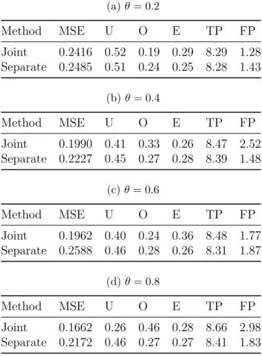
Table 1: Accuracy and variable selection metrics comparing the joint and the sepa-rate PGEE methods, for θ = 0.2,0.4,0.6,0.8, with all covariates shared between the continuous and binary outcomes. Maximum TP is 9.0 and maximum FP is 91.

(a) θ= 0.2 Method MSE U O E TP FP Joint 0.2416 0.52 0.19 0.29 8.29 1.28 Separate 0.2485 0.51 0.24 0.25 8.28 1.43 (b)θ= 0.4 Method MSE U O E TP FP Joint 0.1990 0.41 0.33 0.26 8.47 2.52 Separate 0.2227 0.45 0.27 0.28 8.39 1.48 (c)θ= 0.6 Method MSE U O E TP FP Joint 0.1962 0.40 0.24 0.36 8.48 1.77 Separate 0.2588 0.46 0.28 0.26 8.31 1.87 (d)θ= 0.8 Method MSE U O E TP FP Joint 0.1662 0.26 0.46 0.28 8.66 2.98 Separate 0.2172 0.46 0.27 0.27 8.41 1.83

where βˆ(i) _{is the estimate for the true regression coefficient vector} _β

0 from theith data set. We also computed the absolute bias and the sandwich-formula based standard error for each true non-zero regression coefficient. To compare performance in variable selec-tion, we computed the proportion of data sets in which the methods under-selected (U), over-selected (O) and exactly selected (E) the covariates with true non-zero regression coefficients. (A good variable selection method should have small U and O metrics, and

(45)

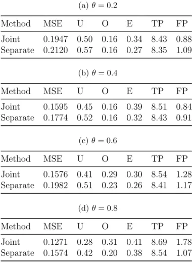
Table 2: Accuracy and variable selection metrics the comparing the joint and the sepa-rate PGEE methods, for θ = 0.2,0.4,0.6,0.8, with some covariates shared between the continuous and the binary outcomes. Maximum TP is 9.0 and maximum FP is 91.

a large E metric). Finally, we calculated the average number of true positives per data set (TP) and the average number of false positives per data set (FP) for both the meth-ods. Table 1 shows the MSE and variable selection metrics for the joint and the separate methods, where all covariates are shared between the bivariate outcomes. We observe that the joint method has smaller MSE than the separate method, with larger gains for the larger values ofθ. Under-selection is usually considered worse than over-selection in

(46)

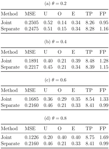
Table 3: Accuracy and variable selection metrics comparing the joint and the sepa-rate PGEE methods, for θ = 0.2,0.4,0.6,0.8, with no covariates shared between the continuous and the binary outcomes. Maximum TP is 9.0 and maximum FP is 91.

variable selection, and we observe that the joint method has a smaller U metric than the separate method for θ = 0.4,0.6,0.8, while its U metric for θ = 0.2 is almost equal to that of the separate method. The joint method also has a larger E metric than the separate method forθ = 0.2 and θ= 0.6, and a similar E metric to the separate method for θ = 0.4 and θ = 0.8. The joint method has a uniformly larger TP metric than the separate method. The tradeoff to this gain is a slightly larger FP metric for the joint

(47)

method, forθ = 0.4 andθ = 0.8. Table 2 shows the metrics for the scenario where some, but not all covariates are shared between the bivariate outcomes. The joint method has smaller MSE, smaller U, larger E, and larger TP than the separate method. It has smaller FP forθ = 0.2 and θ = 0.4, but has larger FP for the larger values of θ. Table 3 shows the metrics for the scenario where no covariates are shared between the bivariate outcomes. Theθ = 0.2 setting under this scenario is the only subcase where the separate method is generally superior than the joint method. However, for larger values ofθ, we see similar trends as described previously.

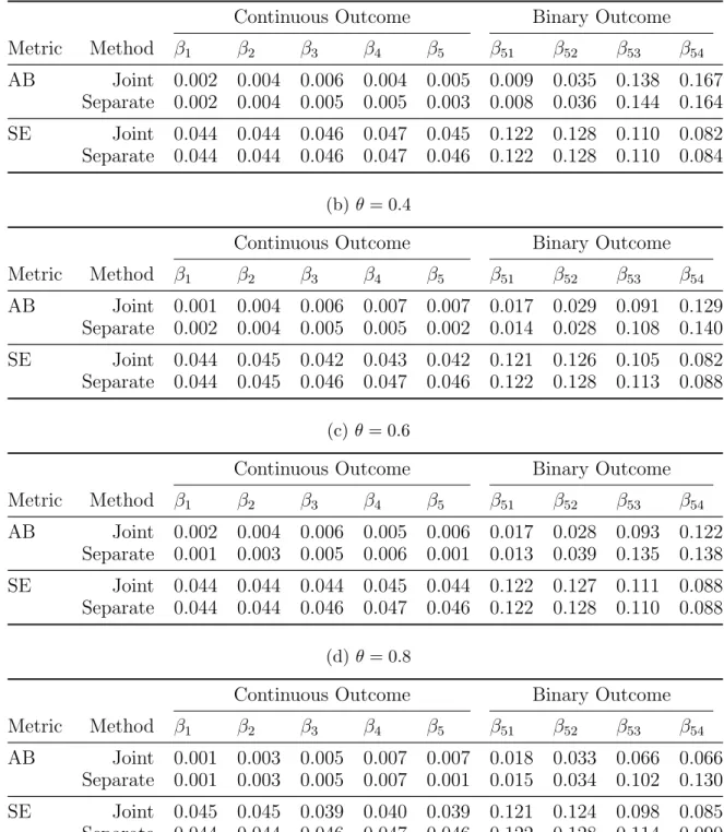
Table 4 shows the absolute bias and the standard errors for the true non-zero coef-ficients for the scenarios corresponding to Table 1. We observe that the absolute bias and the standard errors under both methods are similar for θ = 0.2, while the absolute bias is smaller for most of the binary outcome coefficients for θ = 0.6. For the same covariate setting, but with θ= 0.4 and θ = 0.8, the standard errors are usually smaller for the joint method. For the other scenarios considered (Table 5 and Table 6), the joint and the separate methods perform comparably in terms of absolute bias and standard error for the continuous outcome coefficients, but the joint method is generally superior to the separate method for the binary outcome coefficients.

Overall, we see that the joint method makes gains over the separate method in estimation and variable selection metrics for the binary outcome coefficients, especially

(48)

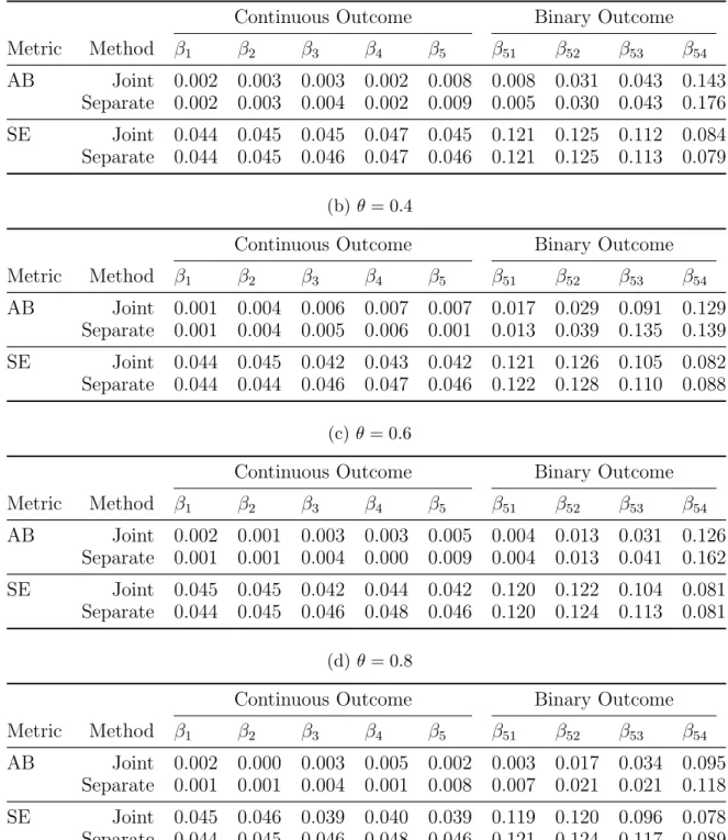
Table 4: Absolute bias (AB) and sandwich-formula based standard errors (SE) of es-timates of true non-zero regression coefficients for the joint and the separate PGEE methods, with all covariates shared between the continuous and binary outcomes.

(a) θ= 0.2

Continuous Outcome Binary Outcome

Metric Method β1 β2 β3 β4 β5 β51 β52 β53 β54 AB Joint 0.002 0.004 0.006 0.004 0.005 0.009 0.035 0.138 0.167 Separate 0.002 0.004 0.005 0.005 0.003 0.008 0.036 0.144 0.164 SE Joint 0.044 0.044 0.046 0.047 0.045 0.122 0.128 0.110 0.082 Separate 0.044 0.044 0.046 0.047 0.046 0.122 0.128 0.110 0.084 (b)θ= 0.4

Metric Method β1 β2 β3 β4 β5 β51 β52 β53 β54 AB Joint 0.001 0.004 0.006 0.007 0.007 0.017 0.029 0.091 0.129 Separate 0.002 0.004 0.005 0.005 0.002 0.014 0.028 0.108 0.140 SE Joint 0.044 0.045 0.042 0.043 0.042 0.121 0.126 0.105 0.082 Separate 0.044 0.045 0.046 0.047 0.046 0.122 0.128 0.113 0.088 (c)θ= 0.6

Metric Method β1 β2 β3 β4 β5 β51 β52 β53 β54 AB Joint 0.002 0.004 0.006 0.005 0.006 0.017 0.028 0.093 0.122 Separate 0.001 0.003 0.005 0.006 0.001 0.013 0.039 0.135 0.138 SE Joint 0.044 0.044 0.044 0.045 0.044 0.122 0.127 0.111 0.088 Separate 0.044 0.044 0.046 0.047 0.046 0.122 0.128 0.110 0.088 (d)θ= 0.8

Metric Method β1 β2 β3 β4 β5 β51 β52 β53 β54

AB Joint 0.001 0.003 0.005 0.007 0.007 0.018 0.033 0.066 0.066

Separate 0.001 0.003 0.005 0.007 0.001 0.015 0.034 0.102 0.130

SE Joint 0.045 0.045 0.039 0.040 0.039 0.121 0.124 0.098 0.085

(49)

for larger values of θ. Intuitively, this makes sense, as the binary outcome coefficients– which are harder to estimate due to the smaller information content of binary outcomes– benefit fromborrowing information from the continuous outcomes. The benefit increases as the strength of association between the outcomes increases.

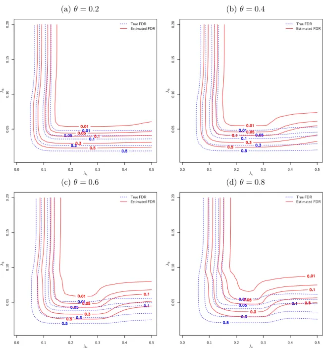
FDR control

For each of 500 data sets generated, we noted the estimated FDR and the true FDR over a 30×30 grid of (λc, λb) values. The smoothed average of these FDRs for θ =

0.2,0.4,0.6,0.8 are plotted in the contour plots in Figure 1. Each level of the contour plots shows the various (λc, λb) combinations which result in the same FDR.

For a particular level of the FDR, our method controls the FDR if the estimated FDR contour lies “above” the true FDR contour. We observe that for all the scenarios, our method is able to control the FDR, albeit a little conservatively for larger values of

θ. For larger values of θ, in the lower right corner of the figures, we also observe that the estimated FDR contours curve upward. This means that for a fixed value of λb, if

λc increases beyond a certain point, the estimated FDR increases. This phenomenon

occurs because for overly large values ofλc, the number of false discoveries in thebinary

coefficients increases, due to the correlation between the outcomes. In practice, this is not a concern, because we choose the optimal (λc, λb) pair using cross-validation, and

our simulation results indicate that the optimal pair of tuning parameters usually does not lie in the lower right corner.

(50)

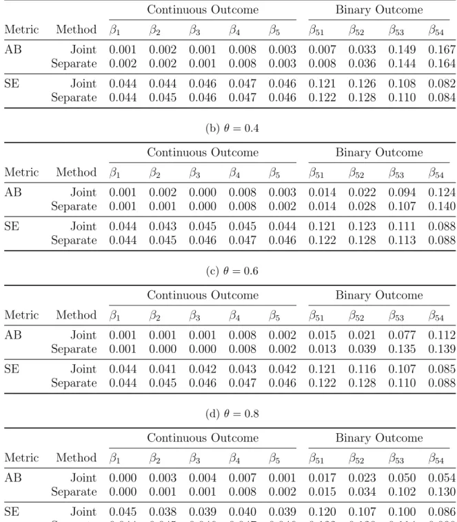
Table 5: Absolute bias (AB) and sandwich-formula based standard errors (SE) of es-timates of true non-zero regression coefficients for the joint and the separate PGEE methods, withsome covariates shared between the continuous and the binary outcomes.

(a) θ= 0.2

AB Joint 0.002 0.000 0.003 0.005 0.002 0.003 0.017 0.034 0.095

Separate 0.001 0.001 0.004 0.001 0.008 0.007 0.021 0.021 0.118

SE Joint 0.045 0.046 0.039 0.040 0.039 0.119 0.120 0.096 0.078

(51)

Table 6: Absolute bias (AB) and sandwich-formula based standard errors (SE) of es-timates of true non-zero regression coefficients for the joint and the separate PGEE methods, with no covariates shared between the continuous and the binary outcomes.

(a) θ= 0.2

AB Joint 0.000 0.003 0.004 0.007 0.001 0.017 0.023 0.050 0.054

Separate 0.000 0.001 0.001 0.008 0.002 0.015 0.034 0.102 0.130

SE Joint 0.045 0.038 0.039 0.040 0.039 0.120 0.107 0.100 0.086

(52)

(a)θ= 0.2 0.0 0.1 0.2 0.3 0.4 0.5 0.05 0.10 0.15 0.20 True FDR_{Estimated FDR} λ_c λb (b)θ= 0.4 0.0 0.1 0.2 0.3 0.4 0.5 0.05 0.10 0.15 0.20 True FDR_{Estimated FDR} λ_c λb (c) θ= 0.6 0.0 0.1 0.2 0.3 0.4 0.5 0.05 0.10 0.15 0.20 True FDR_{Estimated FDR} λ_c λb (d)θ= 0.8 0.0 0.1 0.2 0.3 0.4 0.5 0.05 0.10 0.15 0.20 True FDR_{Estimated FDR} λ_c λb

Figure 1: Contour plots of smoothed true and estimated FDRs. The continuous penalty parameter is on the horizontal axis and the binary penalty parameter is on the vertical axis. Each contour shows the combination of penalty parameters that result in the same true/estimated FDR.

(53)

2.4

MEPS data analysis

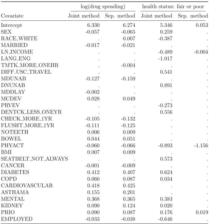
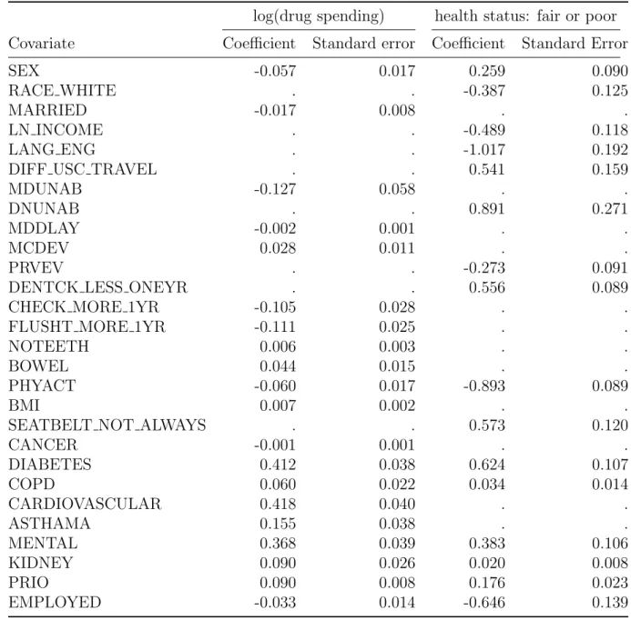
In this section, we demonstrate the application of our PGEE framework and FDR control methodology to data from the Medical Expenditure Panel Survey (MEPS) (https://meps.ahrq.gov/). Our goal is to identify covariates on demographics, medi-cal conditions, income, employment, health insurance coverage, and access to care that are significantly associated with total annual drug spending and health status. We used the 2005 data and restricted attention to Medicare enrollees, 65 years of age and older, with an annual drug spending of $100 or more. We used the natural logarithm of total drug spending as our continuous outcome. As done in Zimmerman (2013), we dichotomized health status into fair or poor (1) and better than fair (0), which formed our binary outcome. We considered a total of 40 covariates, and we used the same set of covariates to model both total drug spending and health status. The complete list of co-variates with descriptions can be found in Table 7. The data set also provides sampling weights for each observation, which we incorporated into the estimation methods. The final data set contains data for 2,953 individuals, who represent 30,146,029 individuals of the U.S. population. We applied both our joint PGEE method as well as separate PGEEs to the responses. Similar to the simulations, four-fold cross-validation was used to select the optimal tuning parameters. Table 8 shows the estimated regression co-efficients under the joint method and under the separate method. Sandwich-formula based standard errors for the regression coefficients from the joint model can be found

(54)

in Table 9. For the continuous outcome–the logarithm of total drug spending–we observe that the joint and separate methods perform similarly in terms of both variable selection and estimation. For the joint model, the covariates with the largest coefficients are CARDIOVASCULAR, DIABETES, and MENTAL, which are binary indicators for the presence of a cardiovascular disease, some form of diabetes, and a mental disease, respectively. Intuitively this makes sense, as pre-existing medical conditions should have strong associations with drug spending.

For the binary outcome–the indicator of fair or poor health status–the joint model is able to detect signal from more covariates than the separate model. This is consistent with the results from our simulation studies, in which the gains in variable selection metrics through joint modeling are primarily made for the binary outcome coefficients. Of course, false discoveries could be a concern here. Hence, we estimated the FDR using the method described in Section 2.2.5 and found it to be 0.07. Interestingly, among all covariates selected by the joint method for the binary outcome, LANG ENG has the largest coefficient in absolute value. The negative coefficient indicates that individuals whose language of comfort is English report better health status than other individuals. The moderate positive coefficient of DIFF USC TRAVEL indicates that individuals who find it difficult to travel to their Usual Source of Care (USC) provider report worse health statuses. Both the joint model and the separate model emphasize the importance of regular physical activity to good health, as seen in the large negative coefficient of PHYACT. In the joint model, the effect of dental health on health status can be seen

(55)

via the coefficients of DNUNAB (individual was unable to receive dental treatment when it was required) and DENTCK LESS ONEYR (frequency of dental checkups are less than once a year). Next, income and employment are positively associated with good health as seen through the negative coefficients of LN INCOME and EMPLOYED. Interestingly, other than DIABETES, most of the variables related to prior medical conditions have relatively small coefficients. SEATBELT NOT ALWAYS has a moderate positive coefficient, indicating that some individuals may have experienced poor health status due to a motor vehicle accident.

Finally, our joint method estimated the association parameter, ρ, to be 0.13. Our simulations indicate that the difference between the copula parameter, θ, and ρ, is roughly 0.10, soθ may be roughly regarded as 0.23.

(56)

Table 7: Covariates used in analysis of MEPS data

Name Type Description

AGEX Continuous Age as of 12/31/2005

SEX Binary Male?

RACE WHITE Binary White?

MARRIED Binary Currently married?

LN INCOME Continuous Shifted natural logarithm of income

LOW INC FAM Binary Low income family?

LANG ENG Binary Primary language spoken at home English?

TMTK MORE ONEHR Binary Takes>1 hour to travel to USC?

DIFF USC TRAVEL Binary Difficult to travel to USC?

DIFF USC PHONE Binary Difficult to reach USC by phone?

MDUNAB Binary Did not receive medical treatment?

DNUNAB Binary Did not receive dental treatment?

PMUNAB Binary Did not receive prescription medication?

MDDLAY Binary Delay in receiving medical treatment?

DNDLAY Binary Delay in receiving dental treatment?

PMDLAY Binary Delay in receiving prescription medication?

MCDEV Binary Covered by Medicaid?

PRVEV Binary Covered by private insurance?

TRIEV Binary Covered by TRICARE?

DENTCK LESS ONEYR Binary Frequency of dental checkups <1/year?

CHOLCK MORE 5YR Binary >5 years since last blood cholesterol check?

CHECK MORE 1YR Binary >1 year since routing medical checkup?

FLUSHT MORE 1YR Binary >1 year since last flu shot?

NOTEETH Binary Lost all natural teeth?

STOOL Binary Has had a blood stool test?

BOWEL Binary Has had sigmoidoscopy/colonoscopy?

PHYACT Binary Mod./vig. physical activity>= 3/week?

BMI Continuous Body Mass Index

SEATBELT NOT ALWAYS Binary Does not always wear a seatbelt?

CANCER Binary Has some form of cancer?

DIABETES Binary Has some form of diabetes?

COPD Binary Has chronic obstructive pulmonary disease?

CARDIOVASCULAR Binary Has a cardiovascular disease?

ARTHRITIS Binary Has arthritis?

ASTHAMA Binary Has asthma?

STOMACH ULCERS Binary Has stomach ulcers?

MENTAL Binary Has a mental disease?

KIDNEY Binary Has a renal disease?

PRIO Count Number of “priority conditions”

(57)

Table 8: Estimated regression coefficients for log(drug spending) and health status out-comes under the joint and the separate PGEE methods. A dot indicates that the covari-ate was not selected by that method, for that outcome. Covaricovari-ates that are not selected by either method are not shown.

log(drug spending) health status: fair or poor

Covariate Joint method Sep. method Joint method Sep. method

Intercept 6.330 6.274 5.346 0.053 SEX -0.057 -0.065 0.259 . RACE WHITE . 0.007 -0.387 . MARRIED -0.017 -0.021 . . LN INCOME . . -0.489 -0.004 LANG ENG . . -1.017 . TMTK MORE ONEHR . -0.004 . .

DIFF USC TRAVEL . . 0.541 .

MDUNAB -0.127 -0.159 . .

DNUNAB . . 0.891 .

MDDLAY -0.002 . . .

MCDEV 0.028 0.049 . .

PRVEV . . -0.273 .

DENTCK LESS ONEYR . . 0.556 .

CHECK MORE 1YR -0.105 -0.132 . .

FLUSHT MORE 1YR -0.111 -0.125 . .

NOTEETH 0.006 0.009 . .

BOWEL 0.044 0.051 . .

PHYACT -0.060 -0.066 -0.893 -1.156

BMI 0.007 0.009 . .

SEATBELT NOT ALWAYS . . 0.573 .

CANCER -0.001 -0.009 . . DIABETES 0.412 0.407 0.624 . COPD 0.060 0.087 0.034 . CARDIOVASCULAR 0.418 0.425 . . ASTHAMA 0.155 0.201 . . MENTAL 0.368 0.365 0.383 . KIDNEY 0.090 0.124 0.020 . PRIO 0.090 0.087 0.176 0.019 EMPLOYED -0.033 -0.038 -0.646 .

(58)

Table 9: Estimated regression coefficients and sandwich formula-based standard errors for covariates selected by the joint method in the MEPS data analysis. A dot in the Coefficient column indicates that the covariate was not selected for that outcome.

log(drug spending) health status: fair or poor

Covariate Coefficient Standard error Coefficient Standard Error

SEX -0.057 0.017 0.259 0.090

RACE WHITE . . -0.387 0.125

MARRIED -0.017 0.008 . .

LN INCOME . . -0.489 0.118

LANG ENG . . -1.017 0.192

DIFF USC TRAVEL . . 0.541 0.159

MDUNAB -0.127 0.058 . .

DNUNAB . . 0.891 0.271

MDDLAY -0.002 0.001 . .

MCDEV 0.028 0.011 . .

PRVEV . . -0.273 0.091

DENTCK LESS ONEYR . . 0.556 0.089

CHECK MORE 1YR -0.105 0.028 . .

FLUSHT MORE 1YR -0.111 0.025 . .

NOTEETH 0.006 0.003 . .

BOWEL 0.044 0.015 . .

PHYACT -0.060 0.017 -0.893 0.089

BMI 0.007 0.002 . .

SEATBELT NOT ALWAYS . . 0.573 0.120

CANCER -0.001 0.001 . . DIABETES 0.412 0.038 0.624 0.107 COPD 0.060 0.022 0.034 0.014 CARDIOVASCULAR 0.418 0.040 . . ASTHAMA 0.155 0.038 . . MENTAL 0.368 0.039 0.383 0.106 KIDNEY 0.090 0.026 0.020 0.008 PRIO 0.090 0.008 0.176 0.023 EMPLOYED -0.033 0.014 -0.646 0.139

(59)

Chapter 3

Fully and empirical Bayes

approaches to estimating

copula-based models for bivariate

mixed outcomes using Hamiltonian

Monte Carlo

3.1

Introduction

As noted in Chapter 1, when measuring the association between correlated outcomes is of primary interest, copula-based models provide a better alternative to GEEs. However, care must be taken when specifying the copula structure for mixed outcomes. Sklar’s Theorem (Sklar, 1959) ensures the uniqueness of a copula only when the marginals are

(60)

continuous. In the burn injury data of Fan and Gijbels (1996), it is of interest to as-sess the association between total burn area (continuous outcome) and survival status

(binary outcome, either dead or survived). When any of the marginals are discrete, the copula is uniquely defined only on the Cartesian product of the ranges of the marginals. Another consequence of having discrete marginals is that dependence measures such as Kendall’s Tau and Spearman’s Rho may now be restricted by the marginal distributions. See Genest and Neˇslehov´a (2007) for more details on the limitations of using copulas with discrete marginals. Song et al. (2009) developed a regression framework for bi-variate mixed outcomes using Gaussian copulas and generalized linear models (GLMs) as marginal models. As they applied the copula directly on discrete marginals, their model suffers from the problems noted above. To avoid these problems, de Leon and Wu (2011) used a latent variable formulation, in which a continuous latent variable is dichotomized to generate the binary outcome. Under this approach, the copula is spec-ified on the continuous outcome and the continuous latent variable, thus avoiding the issues accompanying copulas with discrete margins.

The methods from Song et al. (2009) and de Leon and Wu (2011) are frequentist approaches that use maximum likelihood based techniques for parameter estimation. Indeed, most applications of copulas involve frequentist estimation. However recent advances in Markov Chain Monte Carlo (MCMC) sampling algorithms have enabled Bayesian methods for copula estimation to gain traction. See Silva and Lopes (2008) for an overview of Bayesian copula model estimation and model selection. In the case of

(61)

mixed outcomes, Smith and Khaled (2012) provided a Bayesian framework for copula estimation of mixed outcomes based on data augmentation with latent variables, and provided sampling schemes to perform inference using MCMC. Craiu and Sabeti (2012) extended the latent variable formulation of de Leon and