Fenchel duality-based algorithms for convex
optimization problems with applications in
machine learning and image restoration
Dissertation
submitted in partial fulfillment of the requirements for the academic degree doctor rerum naturalium (Dr. rer. nat.)
by
Andr´e Heinrich
Prof. Dr. Dr. h. c. (NUM) Gert Wanka, Adviser
Fakult¨at f¨ur Mathematik D-09107 Chemnitz
Dipl.-Math. oec. Andr´e Heinrich Technische Universit¨at Chemnitz Fakult¨at f¨ur Mathematik
Bibliographical description
Andr´e HeinrichFenchel duality-based algorithms for convex optimization problems with applications in machine learning and image restoration
Dissertation, 163 pages, Chemnitz University of Technology, Department of Mathematics, Chemnitz, 2012
Report
The main contribution of this thesis is the concept of Fenchel duality with a focus on its application in the field of machine learning problems and image restoration tasks. We formulate a general optimization problem for modeling support vector machine tasks and assign a Fenchel dual problem to it, prove weak and strong duality statements as well as necessary and sufficient optimality conditions for that primal-dual pair. In addition, several special instances of the general optimization problem are derived for different choices of loss functions for both the regression and the classification task. The convenience of these approaches is demonstrated by numerically solving several problems.
We formulate a general nonsmooth optimization problem and assign a Fenchel dual problem to it. It is shown that the optimal objective values of the primal and the dual one coincide and that the primal problem has an optimal solution under certain assumptions. The dual problem turns out to be nonsmooth in general and therefore a regularization is performed twice to obtain an approximate dual problem that can be solved efficiently via a fast gradient algorithm. We show how an approximate optimal and feasible primal solution can be constructed by means of some sequences of proximal points closely related to the dual iterates. Furthermore, we show that the solution will indeed converge to the optimal solution of the primal for arbitrarily small accuracy.
Finally, the support vector regression task is obtained to arise as a particular case of the general optimization problem and the theory is specialized to this problem. We calculate several proximal points occurring when using different loss functions as well as for some regularization problems applied in image restoration tasks. Numerical experiments illustrate the applicability of our approach for these types of problems.
Keywords
conjugate duality, constraint qualification, double smoothing, fast gradient algorithm, Fenchel duality, image deblurring, image denoising, machine learning, optimality condition, regularization, support vector machines, weak and strong duality
Acknowledgments
First of all, I am much obliged to my adviser Prof. Dr. Gert Wanka for supporting me during the last years and giving me the opportunity to work on this thesis. I would like to thank him for many useful hints and input on research issues as well as help on all matters.
I am strongly indebted to Dr. Radu Ioan Bot¸ for his unremitting commitment in providing suggestions and being available for countless enlightening discussions to make this thesis possible. Thank you, Radu, you were the one who got the ball rolling and supported me by demanding to go the extra mile that is required to make things work! Thank you also for being a friend beyond scientific issues! I would like to thank my office mate Dr. Robert Csetnek for useful hints on the thesis, helpful comments and discussions for years.
I am grateful to Prof. Wanka and his whole research group, Christopher, Nicole, Oleg, Radu, Robert and Sorin for the warm-hearted and friendly atmosphere at the department.
It is my duty to thank the European Social Fund and prudsys AG in Chemnitz for supporting my work on this thesis.
Last but not least, I thank Diana for her love, understanding, encouragement and not least for making sacrifices for the purpose of completing this thesis.
Contents
List of Figures ix
List of Tables xi
1 Introduction 1
2 Preliminaries and notions 5
2.1 Convex Analysis . . . 5
2.2 Primal optimization problems . . . 10
2.2.1 Optimization problems in machine learning . . . 10
2.2.2 A general optimization problem . . . 13
2.3 Fast Gradient Algorithm . . . 14
3 Fenchel-type dual programs in machine learning 17 3.1 Duality and optimality conditions . . . 17
3.2 Dual programs for the classification task . . . 25
3.2.1 Hinge loss . . . 25
3.2.2 Generalized hinge loss . . . 26
3.3 Application to image classification . . . 28
3.3.1 Training data . . . 28
3.3.2 Preprocessing . . . 29
3.3.3 Numerical results . . . 30
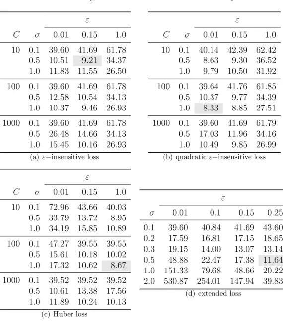
3.4 Dual programs for the regression task . . . 32
3.4.1 The ε−insensitive loss function . . . 33
3.4.2 The quadratic ε-insensitive loss function . . . 34
3.4.3 The Huber loss function . . . 35
3.4.4 The extended loss function . . . 36
3.5 Application to regression tasks . . . 37
3.5.2 Boston Housing data set . . . 41
4 Double smoothing technique for a general optimization prob-lem 43 4.1 Problem formulation . . . 44
4.2 Existence of an optimal solution . . . 45
4.3 Smoothing the general dual problem . . . 47
4.3.1 First smoothing . . . 47
4.3.2 Second smoothing . . . 54
4.4 Applying the fast gradient method . . . 55
4.4.1 Convergence of the optimal objective value . . . 56
4.4.2 Convergence of the gradient . . . 63
4.5 Construction of an approximate primal solution . . . 70
4.6 Convergence to an optimal primal solution . . . 73
5 Application of the double smoothing technique 75 5.1 Application to image restoration . . . 75
5.1.1 Proximal points for the image restoration task . . . 75
5.1.2 Numerical results . . . 82
5.2 Application to support vector regression . . . 90
5.2.1 The double smoothing technique in the case f strongly convex . . . 92
5.2.2 Proximal points for different loss functions . . . 102
5.2.3 SVR Numerical Results . . . 112
A Appendix 119 A.1 Imaging source code . . . 119
A.1.1 Lena test image . . . 119
A.1.2 Text test image . . . 122
A.1.3 Cameraman test image . . . 126
A.2 Support vector regression source code . . . 133
A.2.1 The ε−insensitive loss function . . . 134
A.2.2 The quadratic ε−insensitive loss function . . . 138
A.2.3 The Huber loss function . . . 142
A.2.4 The extended loss function . . . 145
Theses 151
List of Figures
3.1 Example images for the image classification task . . . 29
3.2 Visualization of the scores of the pixels for the classification task 30 3.3 Resulting regression functions . . . 40
3.4 Test errors for the regression task . . . 41
4.1 Fast gradient scheme. . . 55
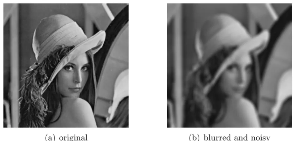
5.1 The Lena test image . . . 83
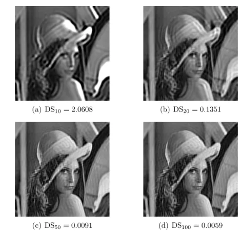
5.2 Restored Lena test image . . . 85
5.3 Plot of objective value and norm of gradient for Lena . . . 86
5.4 The text test image . . . 86
5.5 Restored text test image compared to FISTA . . . 87
5.6 ISNR comparison for text test image . . . 88
5.7 The cameraman test image . . . 89
5.8 Norm of the gradient for 2 and 3 functions in the objective . . . 90
5.9 Primal objective value for 2 and 3 functions . . . 90
5.10 ISNR for 2 and 3 functions in the objective . . . 91
5.11 Plot of sinc function and training data . . . 114
5.12 Regression function for ε−insensitive loss . . . 115
5.13 Regression function for quadraticε−insensitive loss . . . 115
5.14 Regression function for Huber loss . . . 116
5.15 Regression function for extended loss . . . 117
5.16 Norm of the gradient for different loss functions for the regression task . . . 117
List of Tables
3.1 Classification error for the image classification task . . . 31 3.2 Misclassification rates for each loss function for the image
classifi-cation task . . . 32 3.3 Errors for the regression task for each loss function . . . 40
Chapter 1
Introduction
Duality theory plays an important role in the wide field of optimization and its application. Many optimization tasks arising from real world problems involve the minimization of a convex objective function possibly restricted to a feasible set that is convex. Such applications include data mining issues like classification and regression tasks or other fields like portfolio optimization problems (see [24, 39, 75]) or image restoration tasks in the sense of deblurring and denoising (cf. [56, 6]). Suitable methods for solving regression and classification problems originate among others from the field of statistical learning theory and lead to optimization problems involving a loss function and possibly a regularization functional, all of them assumed to be convex functions but not necessarily differentiable. The famous support vector machines approach represents a problem class arising in the field of statistical learning theory in order to solve both regression and classification tasks. This approach has been extensively studied initially by V.N. Vapnik in [71] and [70] where Lagrange duality plays the dominant role in order to obtain dual optimization problems which have structures more easy to handle than the original primal optimization problems that aim at modelling the specific regression or classification task, respectively. A comprehensive study of the theory of support vector machines can be found in [63]. Such methods belong to the class of kernel based methods ([64]) that have become, especially in the last decade, a popular approach for learning functions from a given set of labeled data. They have wide fields of applications such as image and text classification (cf. [30, 45]), computational biology ([54]), time series forecasting and credit scoring (see [47, 68]) and value function approximation in the field of approximate dynamic programming (cf. [65, 49, 10]).
The support vector machines approach is in the main focus of this thesis since it is investigated by means of Fenchel duality other than the common approach using Lagrange duality. Moreover, this concept will be the basis for numerical tests verifying the good performance of the support vector approach with respect to regression and classification problems on the one hand and for the verification
of the applicability of the algorithm developed in this thesis on the other hand. There is a variety of algorithms that numerically solve these optimization prob-lems, each of them more or less designed for special structures of the underlying problem, for example, interior point methods for quadratic convex optimization problems, gradient methods for differentiable problems or subgradient methods for nondifferentiable problems. Compared to other methods, for reasons of good rates of convergence of fast gradient methods often nonsmooth optimization problems are regularized in order to solve them via such gradient methods effi-ciently. Often duality theory is applied since in many cases the dual optimization problem w. r. t. the corresponding primal one has nice properties which allow to numerically solve it in a more easy way. Concerning the famous support vector approach, for example, it is more convenient to solve a Fenchel dual problem or, equivalently, a Lagrange dual problem which may exhibit differentiable quadratic objective functions with simple box constraints or nonnegativity constraints, depending on the chosen loss function. The solution then can be accessed via some well developed algorithms.
In the general setting we consider in this thesis where the primal problem is not assumed to be smooth, we make use of Fenchel duality in addition to a double smoothing technique for efficiently solving the general optimization problem by applying a fast gradient method. In particular, we use a double smoothing technique (see [36]) to be able to apply the fast gradient method introduced in [50] and solve the dual problem. The smoothing is applied since the general dual problem is a non-smooth optimization problem and the fast gradient approach requires a strongly convex, continuously differentiable objective function with Lipschitz continuous gradient.
An important property when solving an optimization problem by means of its dual and obtaining an optimal primal solution is strong duality, namely the case when the optimal primal objective value and the optimal dual objective values coincides and the dual problem has an optimal solution. In general, strong duality can be ensured by assuming that an appropriate regularity condition is fulfilled ([17, 12, 14, 15, 18]). In that case one can also state optimality conditions for primal-dual pairs of optimization problems.
This thesis is structured as follows. Basically it consists of two parts. In the first part a machine learning problem is considered and treated via Fenchel-type duality which is not the common approach in literature for this Fenchel-type of problems. In a second part an approach for solving a general optimization problem approximately is developed and its applicability is demonstrated for two different kinds of application.
In particular, in Chapter 2first some basic notations and results from the field of convex analysis that are used in this thesis are presented. Furthermore, we introduce the optimization problems we will deal with in particular in the
sub-sequent chapters. Section 2.2 introduces these two main optimization problems, where in Subsection 2.2.1, the general optimization problem arising in the con-text of support vector machines for classification and regression (PSV) is derived
from the starting point of the Tikhonov regularization problem and allows for modelling this type of tasks. This primal problem is a more general formulation of the standard optimization problem for support vector tasks in the sense that there is the generalized representer theorem (cf. [62]) underlying the construction of this problem. The generalized representer theorem is a generalization of the well known representer theorem ([74]) and allows the use of regularization terms other than the squared norm of the searched classifier or regression function in the corresponding function space. Another general optimization problem (Pgen)
is then introduced in Subsection 2.2.2. This problem will be extensively studied in Chapter 4. Finally, in Section 2.3 we shortly introduce an algorithmic scheme that will be used for solving (Pgen) via its Fenchel dual problem approximately.
In Chapter 3 we will investigate duality properties between (PSV) and a
Fenchel-type dual problem which will be assigned to it. Therefore, in Section 3.1 we will present weak and strong duality statements and optimality conditions. For a special choice of the regularization term in Section 3.2 we will then derive the particular instances of the primal and dual optimization problems that arise by choosing different loss functions especially designed for the classification task. This is followed by an application of the classification task where we numerically solve a classification task based on high dimensional real world data. In the subsequent Section 3.4 we will calculate the corresponding primal and dual problems for the choice of different loss functions for the regression task and apply the results by solving two different regression tasks numerically. The work done in this chapter is based mainly on [20] and [19].
In Chapter 4 we develop a new algorithm that solves (Pgen), introduced in
Subsection 2.2.2, approximately. In particular, we assign a Fenchel dual problem (Dgen) to (Pgen) and then twice apply a smoothing and solve the doubly smoothed
problem by using a fast gradient scheme with rate of convergence for the dual objective value to the optimal dual objective value of O 1εln 1ε
. Moreover it is shown that the same rate of convergence holds for the convergence of the gradient of the single smoothed dual objective function to zero. After having performed the double smoothing and verified the convergence there will be constructed an approximately optimal primal solution by means of sequences generated by the algorithm and the convergence of this solution to the optimal solution of (Pgen)
is shown.
Having theoretically established the approach for solving (Pgen) in Chapter 4,
we will apply it inChapter 5first to the problem of image restoration which is to solve an ill-posed problem. It is shown that the double smoothing approach developed in Chapter 4 performs well on this problem class and outperforms other methods like the well known fast iterative shrinkage-thresholding algorithm
(FISTA) ([7]) which is an accelerated version of ISTA ([32]). Second, in order to verify its applicability to problems having the sum of more than three functions in the objective, we solve a support vector regression task based on the toy data set that has already been used in Section 3.5.
The thesis concludes with the theses aiming at summarizing the main results of this work.
Chapter 2
Preliminaries and notions
In this chapter we will introduce the basic mathematical background and the-oretical concepts needed in the subsequent chapters. First, in the subsequent section some elementary notions from the field of convex analysis are introduced. In Section 2.2 the optimization problems considered in this thesis are presented. There, we first derive the primal optimization problem that arises in the field of machine learning, namely the support vector machines problem for classification and regression. The presented optimization problem will be extensively studied in Chapter 3 in the view of Fenchel-type duality. In a second subsection therein we state a general optimization problem that will be studied in Chapter 4 also in view of Fenchel-type duality with the focus on an algorithmic scheme which is meant to solve this problem approximately. Finally, the fast gradient method used for numerically solving the smoothed dual problem is presented in the last section of this chapter.
2.1 Convex Analysis
In this section we present notions and preliminaries from convex analysis. It mainly refers to [17] and [5]. For a comprehensive study of the elements of convex analysis we refer also to [58, 40, 77, 37]. In this thesis we restrict ourselves to finite dimensional vector spaces, while the concepts of convex analysis can be found in the mentioned literature in more general settings.
In the whole thesis Rn will denote the n-dimensional real vector space while Rm×n denotes the space of realm×n matrices. The extended real space will be denoted by R:=R∪ {±∞} where we assume by convention (see [17])
(+∞) + (−∞) = (−∞) + (+∞) := +∞, 0·(+∞) := +∞ and 0·(−∞) := 0.
By ei ∈ Rn, i = 1, . . . , n, the i-th unit vector of Rn will be denoted. The nonnegative real numbers are denoted by R+ := [0,+∞). Let U ⊆ Rn be a
subset of Rn. Then the interior of U will be denoted by int(U) and the closure of it by cl(U) whereas the boundary ofU is bd(U) = cl(U)\int(U). The affine hull ofU is defined by aff(U) := ( n X i=1 λixi :n∈N, xi ∈U, λi ∈R, i= 1, . . . , n, n X i=1 λi = 1 )
while the relative interior ofU is defined by
ri(U) :={x∈aff(U) :∃ε >0 :B(x, ε)∩aff(U)⊆U},
where B(x, ε) is the open ball centered atx∈Rn and with radius ε >0. IfU is a convex set and int(U) 6=∅, then int(U) = int(cl(U)) and cl(int(U)) = cl(U). The indicator function δU :Rn →Rof a set V ⊆Rn is given by
δV(x) :=
(
0, if x∈V, +∞, otherwise. For x, y ∈ Rn we denote by hx, yi :=Pn
i=1xiyi the inner product and by kxk the euclidean norm. In the following four different convexity notions for real valued functions will be presented (see [17, 5]).
Definition 2.1. A function f :Rn →
Ris called convex if for all x, y ∈Rn and allλ∈[0,1] it holds
f(λx+ (1−λ)y)≤λf(x) + (1−λ)f(y). (2.1) A function f :Rn →
R is called concave if −f is convex. For a convex set U ⊆Rn a function f :U →
R is called convex onU if (2.1) holds for allx, y ∈U and every λ∈[0,1]. Analogously, a function f is said to be concave onU if −f is convex on U. The extension of the function f to the whole space Ris the function
˜
f :Rn →R, f˜(x) =
(
f(x), if x∈U,
+∞, otherwise. (2.2)
Besides the usual notion of convexity of a function the concepts of strict convexity and strong convexity will play a role in the following.
Definition 2.2. A function f : Rn → R is called strictly convex if for all x, y ∈Rn with x6=y and allλ∈(0,1) it holds
f(λx+ (1−λ)y)< λf(x) + (1−λ)f(y). (2.3) A function f :Rn →R is called strictly concave if −f is strictly convex.
2.1 Convex Analysis
Via the more restrictive concept of uniform convexity, a special case of it, namely strong convexity, is introduced. To do that further notions are required. The domain of a function f : Rn → R is domf := {x ∈ Rn : f(x) < +∞}. A function f : Rn →
R is called proper if f(x) > −∞ for all x ∈ Rn and domf 6=∅.
Definition 2.3. Let f :Rn →Rbe proper. Then f is called uniformly convex with modulus φ:R+→[0,+∞] if φ is increasing, φ(x) = 0 only for x= 0 and
for all x, y ∈domf and all λ∈(0,1) it holds
f(λx+ (1−λ)y) +λ(1−λ)φ(kx−yk)≤λf(x) + (1−λ)f(y) (2.4) Definition 2.4. A proper function f : Rn →
R is called strongly convex if relation (2.4) holds with φ(·) = β2| · |2 for some β >0.
For these four different convexity notions it holds the following. A strongly convex function is also uniformly convex. A uniformly convex function is also strictly convex and a strictly convex function is convex, too. In the subsequent considerations, especially when dealing with the Moreau envelop, we will need the infimal convolution of finitely many functions.
Definition 2.5. The infimal convolution of the functions fi : Rn → R, i = 1, . . . , m, m∈N, is the functionf1. . .fm :Rn→R, (f1. . .fm)(x) := inf xi∈ Rn, Pm i=1xi=x ( m X i=1 fi(xi) ) .
The infimal convolution is called exact atx if the infimum is attained forx∈Rn. In particular, for m= 2, denote f1 = f and f2 = g, the infimal convolution is
given by (fg)(x) = inf y,z∈Rn y+z=x {f(y) +g(z)}= inf y∈X{f(y) +g(x−y)}.
With the help of these notions we introduce an important tool for our analysis in Chapter 4, namely the Moreau envelop of a function (see [5]). We therefore need the notion of lower semicontinuity of a function.
Definition 2.6. A functionf :Rn→Ris called lower semicontinuous at ¯x∈Rn if lim infx→¯xf(x)≥f(¯x). If f is lower semicontinuous at all x∈Rn it is called lower semicontinuous.
It can be shown that the function f is lower semicontinuous if and only if epif is closed, where the set epif :={(x, ξ)∈Rn×
R:f(x) ≤ξ} is called the epigraph of f.
Let f :Rn→
R be proper, convex and lower semicontinuous and γ >0. The Moreau envelop of the functionf of parameter γ is defined as
γf(x) := f 1 2γk · k 2 (x) = inf y∈Rn f(y) + 1 2γ kx−yk 2 . (2.5)
Further we denote by Proxf (x) the unique point in Rn that satisfies
1f(x) = min y∈Rn f(y) + 1 2kx−yk 2 =f(Proxf (x)) + 1 2kx−Proxf(x)k 2
and the operator Proxf :Rn →Rnis called the proximity operator off. Moreover it holds γf(x) =f(Prox γf(x)) + 1 2γkx−Proxγf(x)k 2, where Proxγf (x) = argmin y∈Rn f(y) + 1 2γkx−yk 2
is the unique solution of the minimization problem occurring in (2.5) and is called the proximal point of x. To verify the existence and uniqueness of a minimizer of this problem we refer to [5, Proposition 12.15]. An important property we get from [38, Satz 6.37]. Letf :Rn→R be a proper, convex and lower semicontinuous function andγf :
Rn→Rits Moreau envelop of parameter γ >0. Then γf is continuously differentiable and its gradient is given by
∇(γf) (x) = 1
γ(x−Proxγf (x)) (2.6)
for all x ∈ Rn. A basic concept considering the optimization problems and the formulation of their dual problems studied in this thesis are the concepts of conjugate functions and subdifferentiability. Therefore we next define these notions.
Definition 2.7. The (Fenchel) conjugate function f∗ :Rn → R of a function f :Rn→
R is defined by
f∗(x∗) := sup x∈Rn
{hx∗, xi −f(x)}, (2.7)
while the conjugate fS∗ :Rn →R function of f with respect to the nonempty set S⊆Rn is defined by
fS∗(x) := (f+δS)∗(x) = sup x∈S
2.1 Convex Analysis
The conjugate functionf∗ is convex and lower semicontinuous (see [17, Remark 2.3.1],[37, 77]). For all x∗ ∈ Rn it holds f∗(x∗) = sup
x∈domf{hx, x∗i −f(x)}. Besides the conjugate function we can assign the biconjugate function off, which is defined as the conjugate function of the conjugate f∗, i. e.
f∗∗:Rn→R, f∗∗(x) := (f∗)∗(x) = sup x∗∈
Rn
{hx∗, xi −f∗(x∗)}.
A famous result w. r. t. conjugate functions is the Fenchel-Moreau theorem. Theorem 2.8. Let f :Rn →R be a proper function. Then f =f∗∗ if and only
if f is convex and lower semicontinuous.
For a function f : Rn →
R and its conjugate function the Young-Fenchel inequality holds, i. e. for all x, x∗ ∈Rn we have
f(x) +f∗(x∗)≥ hx∗, xi. (2.8)
Subdifferentiability is essential when studying convex nondifferentiable optimiza-tion problems as is done in the subsequent chapters. Interpreted as a set-valued operator the subdifferential is a maximally monotone operator and leads to special optimization problems arising from the more general formulation of the problem of finding the zeros of the sums of maximally monotone operators (cf. [13]). Next we define the subdifferential of a function at a certain point (see [58, 17, 37, 77]).
Definition 2.9. Let f : Rn →
R be a given function. Then, for any x ∈ Rn with f(x)∈R the set
∂f(x) :={x∗ ∈Rn :f(y)−f(x)≥ hx∗, y−xi ∀y∈Rn}
is said to be the (convex) subdifferential of f at x. Its elements are called subgradients of f atx. We say that the function f is subdifferentiable at x if ∂f(x)6=∅. If f(x)∈/ R we set by convention∂f(x) =∅.
The set-valued mapping∂f :Rn→∂f(x) is called the subdifferential operator of f. If a convex function f : Rn →
R is differentiable at x ∈ Rn then the subdifferential of f at this point coincides with the usual gradient of f atx (cf. [58, Theorem 25.1]). A characterization of the elementsx∗ ∈∂f(x) can be found in [17, Theorem 2.3.12] (see also [77, 37]) which states that
x∗ ∈∂f(x) ⇔ f(x) +f∗(x∗) =hx∗, xi, (2.9) i. e. x∗ ∈∂f(x) if and only if the Young-Fenchel inequality (2.8) is fulfilled with equality.
2.2 Primal optimization problems
In this section we will introduce the primal optimization problems we will deal with in this thesis in Chapters 3 and 4. These problems will be investigated via Fenchel-type duality in the corresponding chapter.
2.2.1 Optimization problems in machine learning
This subsection is dedicated to the derivation of a primal optimization problem occurring in the field of supervised learning methods. These methods are referred to the theory of statistical learning and we will consider especially the support vector machines approach for solving classification and regression tasks.
In the following we will give a brief overview of the concept of reproducing kernel Hilbert spaces in the context of kernel based learning methods. These reproducing kernel Hilbert spaces were first introduced by N. Aronszajn (cf. [2]) in the middle of the last century. A deeper insight into this field can be found for example in [64]. In the context of support vector machines for classification and regression the kernel approach allows finding nonlinear classification or regression functions, respectively, while in its original formulation only linear separation of, for example, different classes of patterns is possible. The following rough illustration of the construction of a reproducing kernel Hilbert space of functions aims at giving the reader an intuitive idea of the basic concept of the approach for establishing an optimization problem for classification and regression tasks. We mainly refer to the description given in [64]. A more common approach to establish the optimization problems that arise in the field of classification and regression tasks is by first introducing the ideas for linear classification and regression in a geometrical sense by means of separating hyperplanes and linear regression hyperplanes. After that, the so-called kernel trick allows for nonlinear classifiers and regression functions, in each case arriving at an optimization problem with linear inequality constraints. For more information on this approach see [46, 73, 42, 26].
Let X be a nonempty set. The function k:X × X →Ris said to be a kernel function if for all x, y ∈ X is satisfies
k(x, y) = hφ(x), φ(y)i,
where φ : X → F is a mapping from X to a so-called inner product feature space. We require k to satisfy the finitely positive semidefiniteness property. The function k satisfies the finitely positive semidefiniteness property if it is a symmetric function and the matrices K = (k(xi, xj))ni,j=1 ∈ Rn×n are positive
semidefinite for all finite subsets X = {x1, . . . , xn} ⊂ X and all n ∈ N. The matrices K are called kernel matrices. It will be now demonstrated how this property characterizes kernel functions, i. e. if a function satisfies the finitely
2.2 Primal optimization problems
positive semidefiniteness property it can be decomposed into a feature map φ into a Hilbert space of functions F applied to both its arguments followed by the evaluation of the inner product in F (cf. [64, Theorem 3.11]). Assume that k :X × X →R is finitely positive semidefinite. We proceed by constructing a feature mapping φ into a Hilbert space for which k is the kernel. Consider the set of functions F = ( r X i=1 αik(·, xi) : r ∈N, xi ∈ X, αi ∈R, i= 1, . . . , r ) . (2.10)
where addition is defined by (f +g)(x) =f(x) +g(x). Since we need an inner product in F we define for two functions f, g ∈ F,
f(x) = r X i=1 αik(xi, x), g(x) = l X i=1 βjk(zi, x),
the inner product to be
hf, gi:= r X i=1 l X j=1 αiβjk(xi, zj). (2.11)
The inner product defined by (2.11) fulfills all the properties required for an inner product (see [64]). Another property, namely the reproducing property of the kernel is also valid,
hk(·, x), fi=f(x).
The two additional properties of separability and completeness are also fulfilled (cf. [64]). Separability follows if the input space is countable or the kernel is continuous. Completeness is achieved, roughly speaking, if one adds all limit points of Cauchy sequences of functions to the set F. We will denote the reproducing kernel Hilbert space associated with the kernel k by Hk. The image of an input xunder the mapping φ:X → Hk is now specified byφ(x) =k(·, x).
Next we derive an optimization problem that arises when a classification or regression task has to be solved based on a set of input patterns X = {x1, . . . , xn} ⊂ X, the corresponding observed values {y1, . . . , yn} ⊂ R and a given kernel functionk:X ×X →Rfulfilling the finitely positive semidefiniteness property. In the case of binary classification tasks the value yi, i = 1, . . . , n, denotes the class label of the corresponding input pattern xi. In that case yi ∈ {−1,1}for example. The aim is to find a functionf ∈ Hkthat appropriately approximates the given training data {(xi, yi) :i = 1, . . . , n} ⊂ X ×R and at the same time is smooth to guarantee that two similar inputs correspond to two similar outputs.
To be able to impose a penalty for predicting f(xi) while the true value is yi, i= 1, . . . , n, we introduce a loss function v :R×R→R that is assumed to be proper and convex in its first variable. There exist many different loss functions to be taken into account, where we will make use of different loss functions in Chapter 3, each of them belonging to the class of loss functions for regression tasks or to the class of loss functions for the classification task. To guarantee smoothness of the resulting function f a smoothing functional Ω : Hk →R is introduced which takes high values for non-smooth functions and low values for smooth ones.
The desired function f will be the optimal solution to the general Tikhonov regularization problem ([67]) inf f∈Hk ( C n X i=1 v(f(xi), yi) + 1 2Ω(f) ) , (2.12)
where C > 0 is the so-called regularization parameter controlling the trade-off between smoothness and accuracy of the resulting classifier or regression function, respectively. Under certain circumstances this would mean to solve an optimization problem in a possibly infinite dimensional space. However, the famous representer theorem (cf. [74]) allows a reformulation of this optimization problem in finite dimension. There, the smoothing functional is of the form Ω(f) = 12kfk2
Hk, wherek · kHk denotes the norm in the reproducing kernel Hilbert
space Hk. However, the starting point for our duality analysis in Chapter 3 will be a more general case by applying the generalized representer theorem stated in [62]. It says that, if g : [0,∞) → R is a strictly monotonically increasing function and we set Ω(f) =g(kfkHk), then for every minimizer f of the problem
inf f∈Hk ( C n X i=1 v(f(xi), yi) +g(kfkHk) ) (2.13)
there exists a vectorc= (c1, . . . , cn)T ∈Rn such that
f(·) = n
X
i=1
cik(·, xi). (2.14)
The coefficients ci are called expansion coefficients and all input points xi for which ci 6= 0 are the so-called support vectors. The existence of such a representation is essential to formulate an equivalent problem for (2.13) which will be the object of investigation via Fenchel-type duality. The normk · kHk induced
by the inner product in the reproducing kernel Hilbert spaceHkintroduced by the inner product (2.11) becomeskfkHk =
p
hf, fi=√cTKcforf ∈ H
2.2 Primal optimization problems
this, from the finite representation we deduce that f(xi) =Pnj=1cjk(xj, xi) = (Kc)i for allxi ∈X. Thus, we can formulate the equivalent optimization problem
(PSV) inf c∈Rn ( C n X i=1 v((Kc)i, yi) +g √ cTKc ) .
In Chapter 3 we will assign a Fenchel-type dual problem to a slightly modified primal problem and investigate duality statements and give optimality conditions. For several different loss functions the dual problems will be derived for both, classification and regression tasks by choosing the function g to beg(·) = 1
2(·) 2
obtaining the standard form of the regularization term in (PSV). Finally, we
numerically solve these dual problems for different tasks. 2.2.2 A general optimization problem
The general optimization problem we consider in this thesis is given by
(Pgen) inf x∈Rn ( f(x) + m X i=1 gi(Kix) ) .
Here, the function f : Rn → R is assumed to be proper, convex and lower semicontinuous. For i = 1, . . . , m the operators Ki : Rn → Rki are assumed to be linear operators. Finally, the functions gi : Rki → R are assumed to be proper, convex and lower semicontinuous functions. Thus, this problem is an unconstrained convex and nondifferentiable optimization problem for which first order methods involving a gradient step are not applicable. In this thesis we will establish an approach that utilizes Fenchel-type duality and a double smoothing technique to solve this problem at least approximately. This allows for applying a fast gradient method (cf. [50]) of rather simple structure and as we will see for a given accuracy ε >0 we will obtain an approximate solution to (Pgen) in
O(1εln 1ε) iterations. For this approach the convergence of the dual objective value and of the norm of the gradient of the single smoothed dual objective can be shown. To obtain a primal solution, we can show that it is possible to construct one by using the sequences of points produced by the fast gradient scheme.
A special case arises when choosing m = 1 in (Pgen). Then this problem
becomes
inf x∈Rn
{f(x) +g(Kx)}, (2.15)
where K : Rn →
Rk is a linear operator, f : Rn → R and g : Rk → R are proper, convex and lower semicontinuous functions. In [13] the authors develop
an algorithmic scheme for solving this problem from a more general point of view. The more general problem there is to find the zeros of sums of maximally monotone operators. This problem is addressed by applying Fenchel-type duality and solve it via a primal-dual splitting algorithm (cf. [3, 4, 55]). In this special case, since∂f :Rn→
Rn and ∂g :Rk →Rk are maximally monotone operators the general algorithmic scheme can be applied where it is possible to show convergence of the sequences of iterates to the optimal solution of the primal problem as well as to the optimal solution of the dual problem, respectively. Notice that in this case the algorithmic scheme in [28] is rediscovered. For the applications we will consider in this thesis it holds thatf ≥0 andg ≥0, which are exactly the assumptions made in [28]. In our setting however we do not ask the functions in the objective to take only nonnegative values.
Having in mind the application of the double smoothing algorithm to image restoration tasks (cf. Section 5.1) we would like to mention here another algorithm that solves a minimization problem having the sum of two functions in the objective, namely the fast iterative shrinkage-thresholding algorithm (FISTA), an accelerated version of ISTA and variants of it (see [7, 11, 32]). In particular, in [7] they solve problems of the form
inf x∈Rn
{f(x) +g(x)} where g : Rn →
R is a convex and continuous function which is allowed to be non-smooth and f : Rn → R is a convex function that is assumed to be continuously differentiable with Lipschitz continuous gradient. This algorithm can be applied to l1−regularization problems having for example the squared
norm function as second component. For this reason we can only compare the performance of the double smoothing algorithm and FISTA for this special choice of functions in Section 5.1. The main work to be done in each iteration there is the computation of the proximal point of the functiong at a certain point (see [7] for details). Therefore, this algorithm belongs to the class of proximal algorithms. In the case m = 1 and f continuously differentiable and strongly convex in (Pgen) we also have to calculate the proximal point of g in each iteration of the
double smoothing algorithm. Nevertheless, we will see that the double smoothing algorithm outperforms FISTA w. r. t. the image restoration task in Section 5.1. There we apply the double smoothing technique in its general version derived in Chapter 4, while it could be accelerated in this setting (see [22]) when having the sum of only two functions in the objective.
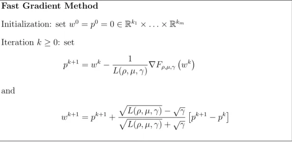
2.3 Fast Gradient Algorithm
In this section we will briefly introduce the gradient algorithm that we will use in Chapter 4 to solve the general optimization problem (Pgen) approximately via its
2.3 Fast Gradient Algorithm
Fenchel-type dual problem. Therefore, consider the unconstrained optimization problem
inf
x∈Rn{f(x)}, (2.16)
where the proper and convex functionf :Rn →R is assumed to be continuously differentiable on Rn with Lipschitz continuous gradient whose Lipschitz constant is L >0. Moreover, we assumef to be strongly convex with parameter γ >0 (see Definition 2.4). These assumptions on f ensure that the algorithmic scheme generates a sequence that converges to a global optimum, i. e. the first order optimality condition is sufficient for a global optimum.
The algorithmic scheme we are applying to solve (2.16) is introduced in [50]. We notice that we deal with a gradient method with constant step size L1. This
Fast gradient scheme Initialization: set y0 =x0 ∈ Rn Iteration k ≥0: set xk+1 =yk− 1 L∇f(y k) yk+1 =xk+1+ √ L−√γ √ L+√γ x k+1−xk
step size is optimal for the gradient method for functions f that fulfill the above properties (see [50, Theorem 2.2.2]). For this algorithmic scheme we get the following estimate (cf. [50, Theorem 2.2.3]),
f(xk)−f∗ ≤min ( 1− r γ L k , 4L (2√L+k√γ)2 ) f(x0)−f∗ +γ 2kx 0−x∗k2 (2.17) where f∗ = f(x∗) is the optimal objective value of f at the optimal solution x∗ ∈Rnof (2.16). Furthermore, for a functionf being continuously differentiable and strongly convex with parameter γ > 0 it holds for all x ∈ Rn (cf. [50, Theorem 2.1.8])
f(x)≥f(x∗) + γ
2kx−x
where x∗ is the unique minimizer for which it holds∇f(x∗) = 0. Therefore, for eachk ≥0 we have γ 2kx k− x∗k2 ≤f(xk)−f∗. (2.19) From (2.17) we get f(xk)−f∗ ≤f(x0)−f∗+γ 2kx 0−x∗k2e−k√Lγ (2.20)
which can be further reformulated by using (2.19), f(xk)−f∗ ≤2f(x0)−f∗e−k
√γ
L. (2.21)
Using (2.21) we get from (2.19) for f having Lipschitz continuous gradient with constantL, γ 2kx k−x∗k2 ≤2(f(x0)−f∗ )e−k √γ L. (2.22)
Since for a convex function f with Lipschitz continuous gradient with Lipschitz constantL >0 it holds for all x, y ∈Rn that
f(x) +h∇f(x), y−xi+ 1
2Lk∇f(x)− ∇f(y)k
2 ≤f(y)
(cf. [50, Theorem 2.1.5]) we obtain by settingy =xk and x=x∗ and by taking into account that∇f(x∗) = 0
1
2Lk∇f(x
k)k2 ≤f(xk)−f∗
. (2.23)
Thus, we obtain an upper bound on the norm of the gradient applying (2.21) given by
k∇f(xk)k2 ≤4L(f(x0)−f∗
)e−k √γ
Chapter 3
Fenchel-type dual programs in
machine learning
In this chapter we investigate the problem (PSV) introduced in Subsection 2.2.1.
Other than in most literature we will not treat this problem based on Lagrange duality (see [46, 63, 69]). We rather employ Fenchel-type duality for such machine learning problems in analogy to the concept in [23] (see also [57]) but the more detailed formulation of the dual problem and the reduction of the dimension of the space of the dual variables compared to the one in [23] make it more suitable for calculations when dealing with concrete loss functions and for numerical implementations. By further reformulating the dual problems we actually solve numerically we obtain the standard form for these problems when applying Lagrange duality.
3.1 Duality and optimality conditions
In this section we will investigate the optimization problem (PSV) derived in
section 2.2.1. The problem (PSV) will be slightly modified to match the general
framework underlying the analysis concerning duality that is done in this section. We define the function ˜g :R→R,
˜ g(t) :=
(
g(t), if t≥0, +∞, otherwise, and introduce the problem
˜ PSV inf c∈Rn ( C n X i=1 v((Kc)i, yi) + ˜g √ cTKc ) .
By assumption the function v : R×R → R is proper and convex in its first variable. Remember that the function g : [0,+∞) → R is assumed to be
strictly monotonically increasing (cf. 2.2.1). Therefore, the problem ˜PSV
is a convex optimization problem which is, depending on the choice of the particular loss function v, not necessarily differentiable. To this problem we assign the Fenchel-type dual problem
˜ DSV sup P∈Rn, P=(P1,...,Pn)T ( −C n X i=1 (v(·, yi)) ∗ −Pi C −g˜∗( √ PTKP) ) . (3.1)
In the following we will prove that weak duality always holds between the primal-dual pair ˜PSV
− D˜SV
and, if a certain qualification condition is satisfied, even strong duality can be assured. The next lemma establishes a certain factorization of a real symmetric and positive semidefinite matrixM ∈Rn×n(cf. [41, Theorem 7.2.6]) which will be used in the proofs of the following two theorems.
Lemma 3.1. Let M ∈Rn×n be a real symmetric positive semidefinite matrix
and let k ≥1be a given integer. Then there exists a unique positive semidefinite
and symmetric matrix B ∈Rn×n such that Bk=M.
By denoting by v P˜SV
andv D˜SV
the optimal objective values of ˜PSV
and ˜
DSV
, respectively, the following theorem states that weak duality always holds between ˜PSV and D˜SV . Theorem 3.2. For P˜SV and D˜SV
weak duality holds, i. e. v P˜SV
≥v D˜SV
.
Proof. Let c ∈ Rn and P = (P
1, . . . , Pn)T ∈ Rn. From the Young-Fenchel inequality we get for alli= 1, . . . , n,
v((Kc)i, yi) + (v(·, yi)) ∗ −Pi C −(Kc)i −Pi C ≥0
and therefore, by summing up the inequalities for alli= 1, . . . , nand multiplying byC > 0, C n X i=1 v((Kc)i, yi) +C n X i=1 (v(·, yi)) ∗ −Pi C + n X i=1 (Kc)iPi ≥0. (3.2)
Again by the Young-Fenchel inequality we have for the function ˜g and its conjugate function ˜g∗
˜
g√cTKc+ ˜g∗√PTKP−√cTKc√PTKP ≥0. (3.3)
Summing up (3.2) and (3.3) we get 0≤C n X i=1 v((Kc)i, yi) +C n X i=1 (v(·, yi)) ∗ −Pi C + n X i=1 (Kc)iPi
3.1 Duality and optimality conditions + ˜g √ cTKc+ ˜g∗√PTKP−√cTKc√PTKP or C n X i=1 v((Kc)i, yi) + ˜g √ cTKc≥ −C n X i=1 (v(·, yi)) ∗ −Pi C −g˜∗ √ PTKP − n X i=1 (Kc)iPi− √ cTKc√PTKP ! (3.4) From Lemma 3.1 we have that there exists a real symmetric and positive semidefinite matrix L∈Rn×n such that K =LL. Furthermore, by applying the Cauchy-Schwarz inequality, we get
PTKc−√cTKc√PTKP = (LP)T(Lc)−p
(Lc)T(Lc)p(LP)T(LP)
=hLP, Lci − kLckkLPk ≤0. Thus, incorporating this observation in (3.4) we finally get
C n X i=1 v((Kc)i, yi) + ˜g √ cTKc≥ −C n X i=1 (v(·, yi))∗ −Pi C −g˜∗ √ PTKP
which means that v P˜SV
≥v D˜SV
.
In order to ensure strong duality between the primal-dual pair P˜SV
and ˜
DSV
we impose the qualification condition
(QC) ImK∩
n
Y
i=1
ri(domv(·, yi))6=∅. (3.5)
Theorem 3.3. If (QC) is fulfilled, then it holds v P˜SV
= v D˜SV
and D˜SV
has an optimal solution.
Proof. First, we define h : Rn →
R, h(x) = (˜g ◦β)(x), where β : Rn → R, β(x) =√xTKx. Furthermore, we definev i :Rn→R, vi(x) :=v(xi, yi), then we have v P˜SV = inf c∈Rn ( n X i=1 Cvi ! (Kc) +h(c) ) .
SinceK is assumed to be positive semidefinite,β(x)≥0 for allx∈Rn and there-fore, domh= Rn andK(domh) =K(
Rn) = ImK. By taking into consideration that dom (Pn
i=1Cvi) =
Qn
i=1dom (v(·, yi)) we have that K(ri(domh))∩ri dom n X i=1 Cvi !! = ImK∩ n Y i=1 ri (domv(·, yi))6=∅.
This means that v P˜SV
<+∞. Taking into account Lemma 3.1 we have that β(x) = √xTKx=p
(Lx)T(Lx) =kLxk is a convex function and so is h. Then
we have that (see [12, Theorem 2.1])
v P˜SV = sup P∈Rn ( − n X i=1 Cvi !∗ (−P)−h∗(KP) ) .
Next we calculate the conjugate function of h. For all z ∈Rn we have from [16] that h∗(z) = (˜g◦β)∗(z) = min q≥0 {g˜ ∗ (q) + (qβ)∗(z)} = min ˜ g∗(0) +δ{0}(z),inf q>0 ˜ g∗(q) +qβ∗ 1 qz . (3.6) Furthermore, β∗(z) = ( 0, if √zTK−z ≤1 andz ∈ImK, +∞, else.
where K− denotes the Moore-Penrose pseudo inverse (cf. [8]) ofK. To see this, consider the following three cases.
(i) Let z ∈ ImK and √zTK−z ≤ 1. Then ∃a ∈
Rn such that z = Ka and
p
(Ka)TK−(Ka) =√aTKK−Ka =√aTKa ≤1. By applying Lemma 3.1 and
the Cauchy-Schwarz inequality, we get β∗(z) = sup c∈Rn n aTKc−√cTKco≤ sup c∈Rn n aTKc−√cTKc√aTKao = sup c∈Rn (La)T(Lc)− kLckkLak ≤0.
The supremum is attained for c= 0 and is equal to 0, i. e. β∗(z) = 0.
(ii) Letz /∈ImK. Then,z can be represented asz =u+Ka, whereu∈KerK, u6= 0, and a∈Rn and β∗(z) = sup c∈Rn n zTc−√cTKco= sup c∈Rn n uTc+aTKc−√cTKco ≥sup t>0 n tkuk2+taTKu−t√uTKuo= sup t>0 tkuk2 = +∞,
since kuk2 >0, Ku= 0 and by settingc:=tu, t >0.
(iii) Let z ∈ ImK and √zTK−z > 1, i. e. ∃a ∈
Rn such that z = Ka and √ zTK−z =√aTKa >1. Then, β∗(z) = sup c∈ n n aTKc−√cTKco≥sup t>0 n taTKa−t√aTKao
3.1 Duality and optimality conditions = sup t>0 n t √ aTKa√aTKa−1o= +∞
and we conclude that β∗ 1 qz = ( 0, if √zTK−z ≤q and z ∈ImK, +∞, else. and h∗(z) = min ˜ g∗(0) +δ{0}(z),inf q>0 ˜ g∗(q) +qβ∗ 1 qz = inf q≥0, q≥√zTK−z, z∈ImK {g˜∗(q)} =− sup q≥0, q≥√zTK−z, z∈ImK {−˜g∗(q)}. Now we have −h∗(KP) = sup q≥0, q≥√PTKP {−g˜∗(q)}. which yields v P˜SV = sup P∈Rn ( − n X i=1 Cvi !∗ (−P)−h∗(KP) ) = sup P∈Rn − n X i=1 Cvi !∗ (−P) + sup q≥0, q≥√PTKP {−˜g∗(q)} = sup P∈Rn q≥0,q≥√PTKP ( − n X i=1 Cvi !∗ (−P)−˜g∗(q) ) . (3.7)
To reformulate the last expression we show that ˜g∗ is monotonically increasing. For allt1, t2 ∈Rsuch that 0≤t1 ≤t2 we observe ˜g∗(t1) = supa≥0{at1−g(a)} ≤
supa≥0{at2−g(a)}= ˜g∗(t2). Now (3.7) becomes
v P˜SV = sup P∈Rn ( − n X i=1 Cvi !∗ (−P)−˜g∗( √ PTKP) )
and that there exists a ¯P ∈Rn (see [12, Theorem 2.1]) such that
v P˜SV =− n X i=1 Cvi !∗ (−P¯)−g˜∗(pP¯TKP¯)
=−C n X i=1 vi !∗ (−1 C ¯ P)−g˜∗(pP¯TKP¯).
As from (QC) we have that ∩n
i=1ri(domvi) =Qni=1ri(domv(·, yi)) 6=∅ it follows (cf. [58, Theorem 16.4]) that there exist ¯Pi ∈
Rn,i= 1, . . . , n, withPni=1P¯i = ¯P, such that n X i=1 vi !∗ −1 C ¯ P = n X i=1 v∗i −1 C ¯ Pi and, therefore, v P˜SV =−C n X i=1 vi∗ −1 C ¯ Pi −˜g∗ v u u t n X i=1 ¯ Pi !T K n X i=1 ¯ Pi ! .
Further, for alli= 1, . . . , nit holds
v∗i −1 C ¯ Pi = sup z∈Rn −1 C ¯ PiTz−v(zi, yi) = ( (v(·, yi)) ∗ −1 CP¯ i i , if ¯Pi j = 0,∀j 6=i, +∞, else.
Since the optimal objective value of P˜SV
is finite, by defining ¯Pi := ¯Pii for i= 1, ..., n, one has Pn i=1P¯ i = ( ¯P 1, . . . ,P¯n)T ∈Rn and v P˜SV =−C n X i=1 (v(·, yi)) ∗ −1 C ¯ Pi −g˜∗pP¯TKP¯,
where ¯P := ( ¯P1, . . . ,P¯n)T. This, along with Theorem 3.2, provides the desired result, ¯P being an optimal solution to D˜SV
.
The next theorem furnishes the necessary and sufficient optimality conditions for the primal-dual pair ˜PSV
- ˜DSV
.
Theorem 3.4. Let (QC) be fulfilled. Then ¯c ∈Rn is an optimal solution for ˜
PSV
if and only if there exists an optimal solution P¯ ∈Rn to D˜
SV such that (i) −P¯i C ∈∂v(·, yi) ((Kc¯)i), i= 1, . . . , n, (ii) ˜g(√c¯TK¯c) + ˜g∗(√P¯TKP¯) = ¯PTK¯c.
3.1 Duality and optimality conditions
Proof. From Theorem 3.3 we get the existence of an optimal solution ¯P ∈Rn to
˜ DSV such that C " n X i=1 v((K¯c)i, yi) + n X i=1 (v(·, yi)) ∗ −1 C ¯ Pi − n X i=1 (K¯c)i −1 C ¯ Pi # + ˜g √ ¯ cTK¯c+ ˜g∗pP¯TKP¯−P¯TKc¯= 0.
By the Young-Fenchel inequality (2.8) we get that the expression in square brackets as well as the three summands on the second line of the above formula are greater or equal to zero. Thus, both of them are zero to fulfill the above equality which is equivalent to
v((K¯c)i, yi) + (v(·, yi)) ∗ −1 C ¯ Pi = (Kc¯)i −1 C ¯ Pi , i= 1, . . . , n, ˜ g √ ¯ cTKc¯+ ˜g∗pP¯TKP¯= ¯PTK¯c, (3.8a)
and we get the optimality conditions (i) and (ii) by regarding the characterization of elements in the subdifferential given by (2.9).
In the following sections we will derive several optimization problems as special instances of ˜PSV
for different choices of loss functions v, each of them designed for the classification or the regression task, respectively. Both cases, however, have in common the choice of the regularization term in ˜PSV
, i. e. the concrete form of the function ˜g :R→Rwhich is specified to be
˜ g(t) = ( 1 2t 2, if t≥0, +∞, else, (3.9)
and corresponds of considering the squared norm of f ∈ Hk as regularization functional, i. e. Ω(f) = 1
2kfk 2
Hk in (2.12), while the particular instance (3.9)
of ˜g in P˜SV
corresponds of choosing g(t) = 12t2 in (P
SV), a commonly used
regularization term in literature. The primal optimization problem associated with this choice of ˜g is now given by
¯ PSV inf c∈Rn ( C n X i=1 v((Kc)i, yi) + 1 2c TKc ) , (3.10)
since √cTKc≥0 for allc∈
Rn. The corresponding dual problem is obtained by considering the conjugate function ˜g∗ of ˜g, which is
˜ g∗(y) = sup x∈dom ˜g {xy−˜g(x)}= ( 1 2y 2, if y≥0, 0, if y <0,
then we have ¯ DSV sup P∈Rn, P=(P1,...,Pn)T ( −C n X i=1 (v(·, yi)) ∗ −Pi C −1 2P TKP ) , (3.11)
since √xTKx ≥ 0 for all x ∈
Rn and for K being a kernel matrix. For this particular instance of the general primal-dual pair ˜PSV
- ˜DSV
clearly strong duality holds as a consequence of Theorem 3.3 when imposing the corresponding regularity condition. The corresponding adapted optimality conditions are stated in the next corollary.
Corollary 3.5. Let (QC) be fulfilled. Then ¯c∈Rn is an optimal solution for
the problem P¯SV
if and only if there exists an optimal solution P¯ ∈Rn to the
problem D¯SV such that (i) −P¯i C ∈∂v(·, yi)((Kc¯)i), i= 1, . . . , n, (ii) K(¯c−P¯) = 0.
Proof. The statement (i) is the same as in Theorem 3.4. We show (ii).
Consid-ering (3.8a) and taking into account the particular choice of ˜g (cf. (3.9)), we have 1 2c¯ TKc¯+1 2 ¯ PTKP¯−P¯TKc¯= 0 which is, since K is a kernel matrix, equivalent to
1 2(¯c−
¯
P)TK(¯c−P¯) = 0. (3.12)
Thus, ¯c−P¯ is a global minimum of the convex function p 7→ 1 2p
TKp, which
means that (3.12) is nothing else thanK(¯c−P¯) = 0.
The case where the kernel matrix K ∈Rn×n is positive definite allows further useful reformulations of the optimality conditions.
Remark 3.6. If K is positive definite, then, due to the fact thatv(·, yi) is proper
and convex for alli= 1, . . . , n, the qualification condition (QC) is automatically fulfilled. Thus, according to Theorem 3.5, ¯c ∈ Rn is an optimal solution for problem ¯PSV
if and only if there exists an optimal solution ¯P ∈Rn to ¯D
SV such that (i) −P¯i C ∈∂v(·, yi)((Kc¯)i),i= 1, . . . , n, (ii) ¯c= ¯P.
3.2 Dual programs for the classification task
Remark 3.7. IfK is positive definite, then the functionc7→ 1
2c
TKcis strongly
convex (on Rn). Consequently, if v(·, y
i), i = 1, . . . , n, is, additionally, lower semicontinuous, the optimization problem ¯PSV
has a unique optimal solution (see, for instance, [38, Satz 6.33]). Further, due to the fact that P 7→ 1
2P
TKP is strictly convex (on Rn), one can see that the dual problem D¯
SV
has at most one optimal solution. This yields, due to Remark 3.6, that whenever K is positive definite and v(·, yi) is lower semicontinuous, for i= 1, ..., n, in order to solve ¯PSV
one can equivalently solve D¯SV
which in this case has an unique optimal solution ¯P, this being also the unique optimal solution of ¯PSV
. In the following sections we will consider the particular instances of primal and dual problems P¯SV
and D¯SV
, respectively, arising with the choice of different loss functions. The particular choice of the regularization term is due to the more easy numerical solvability of the resulting dual optimization problems.
3.2 Dual programs for the classification task
In this section we deal with particular instances of the general model described in Section 3.1 and construct, for three particular loss functions, the correspond-ing dual problems. We apply these three dual problems in order to solve a classification problem on a data set of images, as we will show in Section 3.3. 3.2.1 Hinge loss
The first loss function we consider here is the hinge lossvhl:R×R→R, defined as
vhl(a, y) = (1−ay)+= max{0,1−ay}, (3.13)
which is a proper, convex and lower semicontinuous function in its first component, while (QC) is obviously fulfilled. The primal optimization problem P¯SV
becomes in this case
(Phl) inf c∈Rn ( C n X i=1 1−(Kc)iyi + + 1 2c TKc ) .
To obtain the dual problem (Dhl) of (Phl) for this special loss function, we use
the Lagrange technique in order to calculate the conjugate function of vhl(·, yi), for i= 1, ..., n. For z∈R and i= 1, ..., nwe have
− vhl(·, yi) ∗ (z) = −sup a∈R {za−(1−ayi)+}= inf a,t∈R, t≥0, t≥1−ayi {−za+t} = sup k≥0, r≥0 inf a,t∈R −za+t+k(1−ayi−t)−rt
= sup k≥0, r≥0
inf
a∈R{−za−kayi}+ inft∈R{t−kt−rt}+k
= sup k≥0, r≥0, k+r=1, z+kyi=0 k= sup k∈[0,1], k=−zyi k = ( −zyi, if zyi ∈[−1,0], −∞, otherwise.
Note that in the calculations above we used the fact that the labelsyi,i= 1, . . . , n, can only take the values +1 or−1 for the binary classification task we will consider in Section 3.3. With the above formula we obtain the following dual problem
(Dhl) sup P∈Rn, Piyi∈[0,C], i=1,...,n ( n X i=1 Piyi− 1 2P TKP )
or, by reformulating it as an infimum problem and keeping notation,
(Dhl) inf P∈Rn, Piyi∈[0,C], i=1,...,n ( 1 2P T KP − n X i=1 Piyi ) .
By defining the vectorα= (α1, . . . , αn)T ∈Rn, αi :=Piyi, i= 1, . . . , n, the dual problem can equivalently be written as
(Dhl) inf αi∈[0,C], i=1,...,n ( 1 2 n X i,j=1 αiαjyiyjKij− n X i=1 αi ) ,
a representation which is recognized to be the commonly used form of the dual problem to (Phl) in the literature (see for example [63, 46]).
3.2.2 Generalized hinge loss
Beside the hinge loss, the binary image classification task has been performed for two other loss functions, as we point out in Section 3.3. They both represent particular instances of the generalized hinge lossvughl:R×R→R,
vghlu (a, y) = (1−ay)u+, (3.14) where u > 1. The generalized hinge loss function is proper, convex and lower semicontinuous in its first component, too, while the qualification condition (QC) is again obviously fulfilled. The primal problem to which this loss function gives rise to reads (Pughl) inf c∈Rn ( C n X i=1 (1−(Kc)iyi)u++ 1 2c TKc ) .
3.2 Dual programs for the classification task
To obtain its dual problem we need the conjugate function of vu
ghl(·, yi) for i= 1, ..., n. For allz ∈R and alli= 1, ..., nwe have
− vughl(·, yi)∗(z) =−sup a∈R za−(1−ayi)u+ = inf a,t∈R, t≥1−ayi −za+tu+δ[0,+∞)(t) .
By taking into account that the function t 7→tu+δ[0,+∞)(t) is convex, we can
make again use of Lagrange duality, which provides the following formula for the conjugate of vu ghl(·, yi) fori= 1, ..., n and z ∈R − vghlu (·, yi) ∗ (z) = sup k≥0 inf a∈R, t≥0 −za+tu+k(1−ayi−t) = sup k≥0 inf a∈R
{−za−kayi}+ inf t≥0{t u−kt}+k = sup k≥0, k=−zyi ( (1−u) k u uu−1 +k ) = ( (1−u) −zyi u u−u1 −zyi, if zyi ≤0, −∞, otherwise.
Hence, the corresponding dual problem to (Pughl) looks like
(Dughl) sup Pi∈R, Piyi≥0,i=1...,n ( 1−u (Cuu)u−11 n X i=1 (Piyi) u u−1 + n X i=1 Piyi − 1 2P TKP ) .
Formulated as an infimum problem, (Dughl) becomes
(Dughl) inf Pi∈R, Piyi≥0,i=1...,n ( 1 2P TKP + u−1 (Cuu)u−11 n X i=1 (Piyi) u u−1 − n X i=1 Piyi ) ,
while, by taking α= (α1, . . . , αn)T ∈Rn,αi :=Piyi, i= 1, . . . , n, one obtains for it the following equivalent formulation
(Dughl) inf αi≥0, i=1,...,n ( 1 2 n X i,j=1 αiαjyiyjKij+ u−1 (Cuu)u−11 n X i=1 α u u−1 i − n X i=1 αi ) .
This problem gives rise foru= 2 to
(D2ghl) inf αi≥0, i=1,...,n ( 1 2 n X i,j=1 αiαjyiyjKij+ 1 2C n X i=1 α2i ! − n X i=1 αi )
and for u= 3 to (D3ghl) inf αi≥0, i=1,...,n ( 1 2 n X i,j=1 αiαjyiyjKij + 2 √ 27C n X i=1 α 3 2 i − n X i=1 αi ) ,
which are the situations that we employ, along the one corresponding to the hinge loss, in Section 3.3 for solving the classification task.
Remark 3.8. The problems (Dhl) and (D2ghl) are convex quadratic optimization
problems with affine inequality constraints and they can be solved by making use of one of the standard solvers which exist for this class of optimization problems. This is not anymore the case for (D3ghl), which is however a convex optimization problem. Thus one can use for solving it instead one of the standard solvers for convex differentiable optimization problems with affine inequality constraints. In order to solve both the quadratic and the non-quadratic optimization problems, we applied appropriate optimization routines from the MATLABR optimization toolbox involving interior point methods for convex quadratic optimization problems (see for example [33, 25]).
3.3 Application to image classification
In this section we describe the data for which the classification task, based on the approach described above, has been performed. Furthermore, we illustrate how the data has been preprocessed and give numerical results for the problems (Dhl), (D2ghl) and (D
3
ghl) arising when considering the different loss functions
investigated in Section 3.2. These investigations can be extended by considering other loss functions and by calculating the corresponding dual problems. The only assumption we need for the former is convexity and lower semicontinuity in the first component, which the majority of the popular loss functions (with the exception of the 0−1-loss) fulfill.
3.3.1 Training data
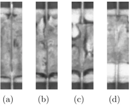
The available data were photographs of components used in the automotive industry, taken by a camera that is an internal part of the machine that produces these items. The overall task is to decide whether a produced component is fine or has to be considered as defective. In particular, a component is considered to be fine if a wire has been brazed correctly onto an attachment and it is defective otherwise. Consequently, a binary classification problem arises, where the label +1 denotes the class of components that are fine and the label −1 denotes the class of components that are defective. In other words, the goal of the classification task is to distinguish good joints from bad joints.
3.3 Application to image classification
There was a total number of 4740 photographs of the components available, represented as gray scale images of size 200×50 pixels. Consisting of 2416 images of class +1 and 2324 images of class −1 the data set was nearly balanced. Since each pixel of the 8-bit gray-scale image represents a specific shade of gray, we assigned to it a value between 0 to 255, where the value equals 0 if the pixel is purely black and 255 if the pixel is purely white, respectively. Figure 3.1 shows four example images, two of each class.
(a) (b) (c) (d)
Figure 3.1: Example images of good ((a), (b)) and bad ((c), (d)) joints.
3.3.2 Preprocessing
In order to be able to use the images for the classification task, we first trans-formed them into vectors. First, each of the images has been represented as a matrix Mt ∈ R200×50, Mt = (mti,j)
200,50
i,j=1 , t = 1, . . . ,4740, with entries
mtij ∈ {0,1, . . . ,255},i= 1, . . . ,200,j = 1, . . . ,50. By simply concatenating the rows of the matrix Mt, we obtained a vector mt representing image t, i. e.
mt= (mt11, . . . , m t 1 200, . . . , m t 50 1, . . . , m t 50 200) T = (mt1, . . . , mt10 000)T ∈R10 000.
Denote by D = {(mt, yt), t = 1, . . . ,4740} ⊂ R10 000 × {−1,+1} the set of all data available. Following [48], the data has been normalized by dividing each data point by the quantity (47401 P4740
t=1 kmtk2) 1
2, due to numerical reasons. Despite the fact that nowadays computations can in fact be performed for 10 000−dimensional vectors, we found it desirable to reduce their dimension to a dimension for which computations can be performed comparatively fast, especially concerning the calculation of the kernel matrix and the value of the decision function. For that reason, a so-called feature ranking was performed, by assigning a score to each pixel indicating its relevance for distinguishing between the two classes. Therefore, for the set of input data D = {m1, . . . , m4740} we
defined the sets
For both of these data sets, we calculated the mean µi, µi(D+) = 1 |D+| X mj∈D+ mji, µi(D−) = 1 |D−| X mj∈D− mji, i= 1, . . . ,10 000,
and the variance σ2i,
σi2(D+) = 1 |D+| X mj∈D+ (mji−µi(D+))2, σi2(D−) = 1 |D−| X mj∈D− (mji−µi(D−))2,
i= 1, . . . ,10 000, fo