Machine learning phases in statistical physics

Copyright by Qi Chen

The Report Committee for Qi Chen

certifies that this is the approved version of the following report:

Machine Learning Phases in Statistical Physics

APPROVED BY

SUPERVISING COMMITTEE:

Timothy H. Keitt, Supervisor Gregory A. Fiete

Machine Learning Phases in Statistical Physics

by

Qi Chen

REPORT

Presented to the Faculty of the Graduate School of The University of Texas at Austin

in Partial Fulfillment of the Requirements

for the Degree of

MASTER OF SCIENCE IN STATISTICS

THE UNIVERSITY OF TEXAS AT AUSTIN August 2017

Acknowledgments

I wish to thank Dr. Tim Keitt for supervising this thesis.

I’d also like to thank Dr. Gregory A. Fiete for supervising my Ph.D work and being in support of my concurrent M.S. in statistics.

I acknowledge Juan Felipe Carrasquilla Alvarez for his very helpful discussion closely related to this report.

Thanks to Vicki, Keller and all my colleagues in Department of Statis-tics and Department of Physics for their help.

Machine Learning Phases in Statistical Physics

Qi Chen, M. S. Stat.

The University of Texas at Austin, 2017

Supervisor: Timothy H. Keitt

ABSTRACT Conventionally, the study of phases in statistical mechan-ics is performed with the help of random sampling tools. Among the most powerful are Monte Carlo simulations consisting of a stochastic importance sampling over state space and evaluation of estimators for physical quantities. The ability of modern machine learning techniques to classify, identify, or in-terpret massive data sets provides a complementary paradigm to the above approach to analyze the exponentially large number of states in statistical physics. In this report, it is demonstrated by application on Ising-type models that deep learning has potential wide applications in solving many-body statis-tical physics problems. In application of supervised learning, we showed that the feed-forward neural network can identify phases and phase transitions in the ferromagnetic Ising model and the convolutional neural network (CNN) is extremely powerful in classifyingT = 0 and T =∞ phases in the Ising gauge model; In application of unsupervised learning, we illustrated that a deep auto-encoder constructed by stacked restricted Boltzmann machines (RBM)

is closely related to the renormalization group (RG) method well understood in modern physics and our reconstruction of Ising spin configurations in the ferromagnetic Ising model is similar to the hand-written digits reconstruction.

Table of Contents

1.3 Deep Learning in statistical physics . . . 4

Chapter 2. Monte Carlo methods in statistical physics 7 2.1 Importance sampling through Markov chains . . . 7

2.2 Monte Carlo for the Ising model . . . 9

2.3 Monte Carlo for the Ising lattice gauge model . . . 11

Chapter 3. Deep learning models 16 3.1 Feed-forward neural network . . . 16

3.1.1 Logistic regression . . . 17

3.1.2 Multi-class classification . . . 18

3.1.3 Multi-layer Perceptron . . . 18

3.1.4 Softmax and cost function . . . 19

3.1.5 Activation functions . . . 19

3.1.6 Backpropagation . . . 20

3.2 Convolutional neural network . . . 21

3.2.1 The Convolution Operation . . . 22

3.2.3 Pooling . . . 23

3.2.4 Full CNN Model . . . 23

3.3 Restricted Boltzmann Machine . . . 24

3.3.1 Bernoulli Restricted Boltzmann machines . . . 25

3.3.2 Maximum Likelihood Learning . . . 25

3.3.3 Contrastive divergence . . . 26

3.4 Deep auto-encoder . . . 27

Chapter 4. Data-preparation and model specification 33 4.1 Ferromagnetic Ising model . . . 33

4.1.1 Data . . . 33

4.1.2 Model . . . 34

4.2 Ising gauge model . . . 35

4.2.1 Data . . . 35

4.2.2 Model . . . 36

Chapter 5. Results 37 5.1 Feed-forward ANN on ferromagnetic Ising model . . . 37

5.2 Deep auto-encoder on ferromagnetic Ising model . . . 39

5.3 CNN on Ising gauge model . . . 42

Chapter 6. Conclusion and discussion 45 Appendix 47 Appendix 1. Sample code 48 1.1 Keras implementation of feed-forward ANN in ferromagnetic Ising model . . . 48

1.2 Keras implementation of CNN in Ising gauge model . . . 52

Bibliography 60

List of Tables

4.1 Sample data frame for L= 20 Ising model. . . 34 5.1 Training and test accuracy for ferromagnetic Ising model. . . . 37

List of Figures

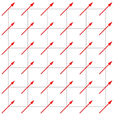
2.1 Ferromagnetic Ising model on the square lattice: Each spin is defined on the site of the lattice and takes binary values from

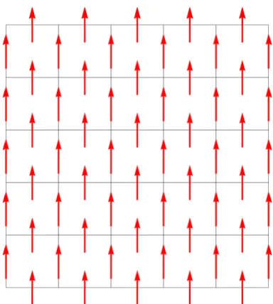
{−1,1}. . . 10 2.2 Ising gauge model on the square lattice: Each spin is defined

on the link of the lattice and takes binary values from {−1,1}. 12 2.3 Non-local flux insertion along x or y direction. . . 14 3.1 The architecture of a feed-forward artificial neural network with

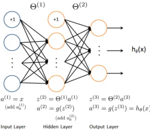
a single hidden layer. The output probabilities of each neuron in the hidden layer are served as inputs for the output layer. (This figure was clipped from online course materials at coursera.com) 30 3.2 The architecture of CNN. The input is a colored picture with a

2d grid of pixels. Two convolution+pooling layers are used to convert pixels into 1d input data for the fully connected layer as in the feed-forward neural network[1]. . . 31 3.3 The architecture of restricted Boltzmann machine: the hidden

units on the top are connected to the visible units at the bottom. There is no internal connections between units in the hidden layer[2]. . . 31 3.4 The architectures of auto-encoders[3]: (a) Auto-encoder with

a single hidden layer and the sigmoid activation function. (b) Deep auto-encoder with stacked RBMs as encoding layers and the decoding layers have the reversed dimensions. . . 32 5.1 The output layer of our trained feed-forward neural network

model averaged over a test set as a function of T/J for the

square-lattice ferromagnetic Ising model of sizeL= 10,20,30,40,60. 38 5.2 The plot for finite size scaling of the critical temperatureTc/J ∼

1/L. The red line is the fitted result. . . 39 5.3 Visualization of effective receptive fields for (a) 100 spins in the

middle layer, (b) 25 spins in the top layer. Each 40 by 40 pixel image depicts the effective receptive field of one of the spins in the hidden units. . . 40

5.4 Loss per data point in the fine tuning stage as a function of number of epochs trained for the deep auto-encoder. The green curve corresponds to random initialization in the model param-eter. The blue curve is initialized with pre-trained model pa-rameters. . . 42 5.5 Reconstructed spin configurations (lower) compared to the

cor-responding raw configurations (upper). . . 43 5.6 The spin flip transformations on the links in x direction every

m plaquettes for L = 20, where m = 2 for the upper row and

m = 4 for the lower row. From left to right: spin configurations before the transformation, spin configurations after the trans-formation, spins changed under the transformation indicated by the white spots. . . 44

Chapter 1

Introduction

In this chapter, we introduce the basic knowledge about statistical physics[4] and machine learning[5], which motivates our work on specific mod-els. In 1.1 we present the basic knowledge of statistical physics. In 1.2 we introduce the basics of machine learning. In 1.3, we address our motivation for the work on deep learning application in statistical physics and the orga-nization of following chapters.

1.1

Statistical Physics

Statistical physics is a branch of physics that uses methods of proba-bility theory and statistics, and particularly the mathematical tools and nu-merical techniques for dealing with large populations and approximations, in solving physical problems. It can describe a wide variety of fields with an inherently stochastic nature.

In particular, statistical mechanics develops the phenomenological re-sults of thermodynamics from a probabilistic examination of the underlying microscopic systems. It provides a framework for relating the microscopic properties of individual atoms and molecules to the macroscopic or bulk

prop-erties of materials that can be observed in every day life, therefore explain-ing thermodynamics as a natural result of statistics, classical mechanics, and quantum mechanics at the microscopic level.

One of the most important equations in Statistical mechanics is the definition of the partition function Z, which is essentially a weighted sum of all possible statesq available to a system:

Z =X

q

exp(−E(q)/kBT), (1.1)

where kB is the Boltzmann constant, T is temperature and E(q) is energy of

state q.The probability of a given state q is usually decided by the energy of state q and also the temperature:

P(q) = exp(−E(q)/kBT)

Z . (1.2)

The macroscopic observableO’ s are weighted averages of microscopic degrees of freedoms associated with q’s:

<O>=X

q

P(q)O(q). (1.3)

In classical systems, phases of matters are characterized by so called order parameters–the weighted averages of particular choices of physical observ-ables, e.g. magnetic moment. Phase transitions happen when there is an abrupt change in the order parameter as a function of temperature. Although some phase transition problems in statistical physics can be solved analytically using approximations and expansions, most current research utilizes the large

processing power of modern computers to simulate or approximate solutions. A common approach to statistical problems is to use a Monte Carlo simulation to yield insight into the dynamics of a complex system.

1.2

Machine Learning

Machine learning lives in the cross field between statistics and computer science, exploring the study and construction of algorithms that can learn from and make predictions on data. Machine learning is employed in a range of computing tasks where designing and programming explicit algorithms with good performance is difficult or infeasible; example applications include email filtering, detection of network intruders or malicious insiders working towards a data breach, optical character recognition (OCR), learning to rank, and computer vision.

Machine learning can be supervised or unsupervised depending on whether the desired outputs are given or not. The goal of supervised learning is to learn a general rule that maps inputs to outputs, whereas unsupervised learning can be used to discover hidden patterns or as a means towards an end such as fea-ture selection. Within the field of data science, machine learning is a method used to devise complex models and algorithms that lend themselves to predic-tion.

In particular, deep learning is the application to learning tasks of arti-ficial neural networks (ANNs) that contain more than one hidden layer. It is a class of machine learning algorithms that:

1. use a cascade of many layers of nonlinear processing units for feature extraction and transformation. Each successive layer uses the output from the previous layer as input. The algorithms may be supervised or unsupervised and applications include pattern analysis (unsupervised) and classification (supervised).

2. are based on the (unsupervised) learning of multiple levels of features or representations of the data. Higher level features are derived from lower level features to form a hierarchical representation.

3. are part of the broader machine learning field of learning representations of data.

4. learn multiple levels of representations that correspond to different levels of abstraction; the levels form a hierarchy of concepts.

Deep learning has been a rising part of machine learning methods based on learning data representations, as opposed to task specific algorithms. The architectures of deep learning includes deep neural networks, deep belief net-works and recurrent neural netnet-works that having been widely applied to fields including computer vision, speech recognition, natural language processing, etc.

1.3

Deep Learning in statistical physics

Conventionally, the study of phases in statistical mechanics is per-formed with the help of tools that have been carefully designed to elucidate

the underlying configurations of various states. Among the most powerful are Monte Carlo[15] simulations consisting of a stochastic importance sam-pling over state space, and the evaluation of estimators for physical quantities calculated from samples. Machine learning, already explored as a tool in condensed-matter research[7, 6, 13, 12, 9, 16, 14], provides physicists a com-plementary paradigm in analyzing exponentially large data sets embodied in the state space of statistical physics models. In this report, we closely followed the work by Juan[7], Pankaj[14] and applied deep learning models in studying phases of matter based on data sets sampled by Monte Carlo simulations. We first demonstrated the power of supervised feed-forward artificial neural net-work (ANN) in the classification of phases in the prototypical example of the square-lattice ferromagnetic Ising model. Then we turned to a more compli-cated example of Ising gauge model and examined the ability of convolutional neural network (CNN) to detect phase transitions through the local constraints in the flux through a plaquette. Finally, we showcased the power of deep auto-encoders consisting of multiple layers of restricted Boltzmann machine (RBM) in reconstructing spin configurations in the microscopic states of ferromagnetic Ising model close to the critical point of phase transition.

This report is organized as follows. In chapter 2, we introduce the Markov chain Monte Carlo sampling method with the Metropolis algorithm and its application in two prototypical statistical physics models: ferromag-netic Ising model and Ising gauge model. In Chapter 3, feed-forward ANN and CNN are reviewed and specified in our application. In addition, deep

auto-encoders and their building blocks–RBMs are introduced as an ANN for unsupervised learning. We point out the intimate relationship between renor-malization group methods and RBM and specified the details of stacked RBMs in encoding and decoding spin configurations in ferromagnetic Ising models. In Chapter 4, we elaborate our data preparation process and specify the hyper-parameters in our models. In Chapter 5 we report our training and testing results for both supervised and unsupervised learning. Conclusions and further discussions are made in Chapter 6.

Chapter 2

Monte Carlo methods in statistical physics

The Monte Carlo method is a traditional numerical tool for simulating classical many-particle systems by introducing artificial dynamics based on ’random’ numbers. For our purposes, we will use Monte Carlo sampling to generate spin configurations data for the Ising type models. We will first introduce the Metropolis algorithm in the Markov chain Monte Carlo method and then apply it to both the ferromagnetic Ising model and the Ising gauge model.

2.1

Importance sampling through Markov chains

In this section, we explain the importance sampling method for clas-sical many-particle systems in the canonical (N, V, T) ensemble[17]. When calculating averages in the (N, V, T) ensemble, the configurationX should be weighted according to the Boltzmann factor

ρ(X)∝exp[−βE(X)], β = 1

kBT

(2.1) This suggests that we apply Monte Carlo integration with importance sam-pling. However, as the number of configurations with a particular energy in-creases exponentially, most of the randomly constructed states have very high

energy-hence for finite temperature they will be accepted with a vanishingly small probability and we spend most of our time generating configurations which are then rejected. As a result, importance sampling becomes very inef-ficient. To improve efficiency in sampling, the configurations are constructed through a Markov chain, in which each new configurationX0 is generated with a probability distribution depending on the previous configuration X given by

T (X →X0). Then the probability of having a sequence of objectsXi becomes

PN(X1, X2, . . . , XN) =P1(X1)T (X1 →X2)T(X2 →X3). . . T (XN−1 →XN).

(2.2) In our problem, we want to generate a Markov chain of system configurations such that they have a distribution proportional to exp[−βE(X)]. In other words, we want to find a transition probability T (X →X0) which leads to a given stationary density ρ(X). This is achieved by the Metropolis Monte Carlo method, in which T (X →X0) is constructed as

T (X→X0) =ωXX0A_XX0, (2.3)

whereωXX0 is the proposal distribution andA_XX0 is the acceptance probability.

Asρ(X) is the stationary distribution, we want

T (X →X0)ρ(X) = T (X0 →X)ρ(X0). (2.4) By inserting Eq. (3) into Eq. (4), one finds

ωXX0A_XX0ρ(X) = ω_X0_XA_X0_Xρ(X0) ⇒ AXX0 AX0_X = ωX0Xρ(X 0₎ ωXX0ρ(X) . (2.5)

In the Metropolis procedure, the acceptance criterion for an attempted move X→X0 is given by AXX0 = min 1,ωX0Xρ(X 0₎ ωXX0ρ(X) (2.6)

2.2

Monte Carlo for the Ising model

The Hamiltonian (i.e. energy) of the ferromagnetic Ising model defined on theL×L square lattice (Fig. 2.1) is given as:

H =−J X

<ij>

S_izS_jz, (2.7)

where the Ising spins Sz

i live on the sites of a two-dimensional square lattice

and takes binary values from{−1,1}. In total, we have N =L×L sites and 2N _{states. This is a textbook model in classical statistical mechanics which}

describes the phase transition from ferromagnetic (FM) phase (|< Sz

i >| ≈1)

at low temperatures to paramagnetic (PM) phase (| < Sz

i > | ≈ 0) at high

temperatures. In order to formulate the Metropolis procedure, we must make a choice for ωXX0. For the two-dimensional Ising model on an L×L square

lattice, we can take

ωXX0 =

(

1 /L2 if X and X0 differ by one spin

0 otherwise . (2.8)

In order to generate a trial configuration, one can select a spin at random and the trial configuration is the present configuration with the selected spin turned over. The energy difference is given by

Figure 2.1: Ferromagnetic Ising model on the square lattice: Each spin is defined on the site of the lattice and takes binary values from {−1,1}.

On the square lattice in two dimension, it is clear that the energy difference depends only on the number of neighbors which have the same spin as the selected spin in the old configuration - between 0 and 4. the energy differences are        

∆E(X →X0) # of neighbors with the same spin

−8J 0 −4J 1 0 2 4J 3 8J 4         . (2.10)

The trial state is accepted with probability:

AXX0 =

(

exp (−β∆E(X →X0)) if ∆E(X →X0)>0

1 else (2.11)

Since exp (−β∆E(X →X0)) can assume only five different values, it is advis-able to store these in an array in order to avoid calculating the exponential function over and over again. Notice that the average number of steps between two updates of the same spin is equal toL2_{. Therefore, the Monte Carlo steps} per spin(MCS) is equal to L2 _{trials. (Remark: The initial configuration will} be chosen either random or as FM (all spins taking either +1 or −1).) The specific heat is calculated according to

CV = 1 kBT2 ∂2Log[Z] ∂β2 = 1 kBT2 " P Xe −βH(X)_H2_(X) P Xe −βH(X) − P X e −βH(X)_H(X) P Xe −βH(X) 2# = 1 kBT2 E2_NVT− hEi2 NVT . (2.12)

Similarly, the magnetic susceptibility can be written as

χ=βM2− hMi2

. (2.13)

2.3

Monte Carlo for the Ising lattice gauge model

The Hamiltonian for the Ising gauge model[8] (Fig. 2.2) is

H =−JX

p

Y

i∈p

σ_iz, (2.14)

where the Ising spins live on the bonds of a two-dimensional square lattice with plaquettes p and takes binary values from {−1,1}. This model has a

Figure 2.2: Ising gauge model on the square lattice: Each spin is defined on the link of the lattice and takes binary values from{−1,1}.

gauge symmetry, i.e. the Hamiltonian is invariant under the following trans-formation:

˜

σ_ijz =wiσzijwj (2.15)

wherewi =±1. We can count the number of states in the Ising gauge theory

on a finite square lattice with periodic boundary condition as follows: If the lattice hasN sites, then it has 2N nearest-neighbor links. Thus there are 22N

different σ_ijz configurations. On the other hand, there are 2N different gauge transformations, which induces 2N2 different gauge-equivalent classes. If we

choose to label those classes by plaquette values, one naively expects that different plaquette configurations will provide 2N _{different labels. However,}

the plaquette values are not independent under periodic boundary condition. They satisfy Y p Y i∈p σ_iz = 1 (2.16)

So they only provide 2N2 states. As a result, each plaquette configuration corresponds to four different states. To see this (Fig. 2.3), we consider the dashed line along x or y direction where all vertical links are flipped, which gives rise to the same plaquette configurations but they are gauge inequivalent because they correspond to inserting a differentZ2 flux through the two holes in the torus. Therefore, 2N

2 different flux configurations plus the four-fold degeneracy allow us to recover 2×2N _{states[8]. Similar to FM Ising model, in}

order to formulate the Metropolis procedure, we must make a choice forωXX0.

Notice that in two dimension, there are 2×N bonds for N sites. Thus

ωXX0 =

(

1/2L2 _{if X and X}0 _{differ by one spin on one link}

0 else . (2.17)

The step of generating a trial configuration is again to select a spin at random, and the trial configuration is the present configuration with the selected spin turned over. The energy difference is given by

Figure 2.3: Non-local flux insertion along x or y direction.

On the square lattice in two dimension, it is clear that the energy difference depends only on the neighboring plaquettes flux:



  

∆E(X →X0) neighboring plaquettes flux

−4J (−1,−1) 0 (−1,1) or (1,−1) 4J (1,1)     . (2.19)

The trial state is accepted with probability:

AXX0 =

(

exp (−β∆E(X →X0)) if ∆E(X →X0)>0.

1 otherwise. (2.20)

Since exp [−β∆E(X →X0)] can assume only 3 different values, it is advisable to store these in an array in order to avoid calculating the exponential function over and over again. The average number of steps between two updates of the

same spin is equal to 2L2_{. Therefore, the Monte Carlo steps per spin (MCS)} is equal to 2L2 _{trials. However, the above procedure will not work for T →0} corresponding to the strong coupling limit (J → ∞) as a single spin flip will cost infinite energy. To keep the chain moving, the most natural choice is to given the system the possibility of performing both single spin flips and local gauge transformations[18]. The relative number of both types of excitations may be chosen freely. With this in mind we choose ωXX0 as:

ωXX0 =      s 2L2 X local → X0 2(1−s) 2L2 X gauge → X0 0 otherwise . (2.21)

Our choice is based on the fact that there areL2 _{gauge updates and 2L}2 _single spin flips.

Chapter 3

Deep learning models

In this chapter, we introduce the essential deep learning tools applied to our models. In 3.1, feed-forward ANN is introduced. In 3.2, we address the practical aspects of the convolutional neural network without getting bogged down in the theoretical details. In 3.3, the restricted Boltzmann machine is in-troduced with contrastive divergence as an approximation in gradient descent. In 3.4, we illustrate the structure of the deep auto-encoder based on stacked RBMs and point out the necessity of pre-training.

3.1

Feed-forward neural network

Feedforward ANN (Fig. 3.1) has been widely applied in multi-class clas-sification problems, which is based upon multiple hidden layers with logistic hidden units. We first introduce the logistic regression in binary classifica-tion, then we generalize it to multi-class classification problems. With this building block, one can construct multi-layer perceptrons in a deep neural network and the predicted probabilities in the output layer are given by the softmax function. Alternatively, different activation functions can be used to construct hidden units. To achieve the minimization of the cost function, we

introduce the backpropagation method in evaluating the gradient descent of a deep neural network.

3.1.1 Logistic regression

The basic model for binary classification is the logistic regression based on the sigmoid function:

hθ(x) = g(xθ) =

1

1 +e−xθ, (3.1)

where the input variablexis an n-dimensional vector andθis the weight vector for binary classification:

x= (x1, x2, . . . , xn), θ =      θ1 θ2 .. . θn      , (3.2)

The learning goal is to maximize the log likelihood function:

J(θ) = m X i=1 y(i)loghθ x(i) + 1−y(i)log 1−hθ x(i) , (3.3)

where the subscript (i) labels the cases from 1 to m. The gradient ascent is based on ∂J(θ) ∂θj =− m X i=1 hθ x(i) −y(i)x(_ji) (3.4) To prevent overfitting for data, one can addL2 regularization to penalize large magnitude of weights, J(θ) = m X i=1 y(i)loghθ x(i) + 1−y(i)log 1−hθ x(i) − λ 2 n X j=1 θ2_j, (3.5)

∂J(θ) ∂θj =    −Pm i=1 hθ x(i) −y(i) x(_ji), j = 0 − m P i=1 hθ x(i) −y(i) x(_ji)−λθj, j ≥1 , (3.6)

where λ >0 is the regularization parameter. 3.1.2 Multi-class classification

The logistic regression can be easily generalized to one-vs-all classifi-cation problems. Suppose we have K classes in our dataset, the model pa-rameters will be a matrix Θ ∈RK×(N+1)_{, where each row corresponds to the} learned logistic regression parameters for one class. When training the classi-fier for class k ∈ {1,..., K}, one will want a m-dimensional vector of labels y, where yj ∈ 0,1 indicates whether the j-th training instance belongs to class

k(yj = 1), or if it belongs to a different class (yj = 0).

3.1.3 Multi-layer Perceptron

Multi-layer Perceptron (MLP) is a supervised learning algorithm that learns a functionf :Rn_→RK _{by training on a dataset, wherenis the number}

of dimensions for input and K is the number of dimensions for output. Given a set of features X ={x1, x2,..., xn} and a target y, it can learn a non-linear

function approximator for either classification or regression. It is different from the logistic regression, in that between the input and the output layer, there can be one or more non-linear layers, called hidden layers.

3.1.4 Softmax and cost function

If there are more than two classes, the output function would be a vector of size K(number of classes). Instead of passing through logistic function, it passes through the softmax function in order to keep the summation of predicted probabilities to be equal to 1. The softmax function is defined as

softmax(z)i =

exp (zi)

PK

l=1exp (zl)

, (3.7)

wherezirepresents thei-th element of the input to softmax, which corresponds

to class i. The result is a vector containing the probabilities that sample x

belong to each class. The output is the class with the highest probability. The cost function for K classes, m training examples and L layer neural network is given by J(θ) = −1 m " _m X i=1 K X k=1 y_k(i)log hθ x(i) k +1−y(_ki)log 1−hθ x(i) k # + λ 2m L−1 X l=1 sl X i=1 sl+1 X j=1 θ(_ijl)2, (3.8)

where sl is the number of nodes in layer l. Notice that the feature label is

from 0 ton, so s1 =n, sL =K, and

x(i) =x(₀i), x₁(i), . . . , x(_nn), i= 1, . . . , m (3.9) withx(₀i)= 1.

3.1.5 Activation functions

1. Logistic Sigmoid: g(z) = _1+exp(1 _−z),

2. Rectified Linear Units (ReLu): g(z) = max{0, z}, 3. Hyperbolic Tangent: g(z) = tanh(z).

As generalized from the logistic regression, the logistic sigmoid function has a gradient easy to compute: g0(z) = (1−g(z))g(z) and is widely used in feed-forward ANN. ReLu is particularly useful in extracting the non-linear features in the convolutional neural network that will be discussed in the next section. 3.1.6 Backpropagation

The forward propagation for each training example is given by

a(i)(1) =x(i), z(i)(2) =θ(1)a(i)(1), a(i)(2) =g z(i)(2),add a(₀i)(2) .. . a(i)(L−1) =g z(i)(L−1), z(i)(L) =θ(L−1)a(i)(L−1), a(i)(L) =g z(i)(L). (3.10)

We could define the error of nodej in layerl asδ(_ji)(l), then by considering the sigmoid activation function,

δ(i)(L) =a(i)(L)−y(i), δ(i)(L−1) =hg z(i)(L−1) 1−g z(i)(L−1).∗ θ(L−1)Ti sL−1×K δ(i)(L), .. . δ(i)(l+1) =hg z(i)(l+1) 1−g z(i)(l+1).∗ θ(l+1)Tiδ(i)(l+2) (3.11) where sl is the number of units in layer l. A tedious calculation of gradients

gives rise to the result ∂J(θ) ∂θ(l) = 1 m m X i0₌₁ δ(i0)(l+1)a(i0)(l) T + λ mθ (l) _(3.12)

3.2

Convolutional neural network

Convolutional networks, also known as convolutional neural networks or CNNs, are a specialized kind of neural network for processing data that has a known, grid-like topology[10]. Examples include time-series data, which can be thought of as 1D grid taking samples at regular time intervals, and image data, which can be thought of as a 2D grid of pixels. Convolutional networks are simply neural networks that use convolution in place of general matrix multiplication in at least one of their layers.

3.2.1 The Convolution Operation

The convolution operation on continuous functions is defined as

s(t) = (x∗w)(t)≡

Z

x(a)w(t−a)da. (3.13) In the discrete version, integration is replaced by summation:

s(t) = (x∗w)(t)≡

∞ X

a=−∞

x(a)w(t−a). (3.14) The first argument x is referred to as the input and the second argument w

is named the kernel. The output is sometimes referred to as the feature map. In the machine learning applications, the input is usually a multi-dimensional array of data and the kernel is usually a multi-dimensional array of parameters that are adapted by the learning algorithm. We will refer to these multidi-mensional arrays as tensors. Notice that both kernels and input are finite dimensional in practice. For convolution more than 1 axis, we have

s(i, j) = (I∗K)(i, j) =X

m

X

n

I(m, n)K(i−m, j −n). (3.15) It is noticeable that the convolution operation is commutative:

s(i, j) = (K∗I)(i, j) =X m X n I(i−m, j−n)K(m, n). (3.16) 3.2.2 Motivation

Convolution leverages three important ideas that can help improve a machine learning system: sparse interactions, parameter sharing and equiv-ariant representations. Sparse interaction is achieved by making the kernel

smaller than the input. In a deep convolutional neural network, units in the deeper layers may indirectly interact with a larger portion of the input. This allows the network to efficiently describe complicated interactions between many variables by constructing such interactions from simple building blocks that each describe only sparse interactions. Parameter sharing refers to using the same parameter for more than one function in a model. The particular form of parameter sharing in the case of convolution causes the layer to have a property called equivariance to translation, which means if the input changes, the output changes in the same way. The mathematical definition is given by

f(g(x)) =g(f(x)) (3.17) whereg can be any function that translates the input.

3.2.3 Pooling

A pooling function replaces the output of the net at a certain location with a summary statistic of the nearby outputs. For example, the max pooling operation reports the maximum output within a rectangular neighborhood. In all cases, pooling helps to make the representation become approximately invariant to small translations of the input.

3.2.4 Full CNN Model

The full architecture (Fig. 3.2) of the CNN model consists of

1. Convolution layer: comprised of feature maps due to multiple feature detectors as Input⊗Feature detector = Feature Map,

2. ReLu layer: creating nonlinear features by using rectified linear units, 3. Max pooling layer: pooling the maximum in the window,

4. Flattening: converting pooled feature map into 1-d array, which serves as input layer of feedforward neural network,

5. Full connection: feedforward neural network training.

In more sophisticated applications, one can include multiple sets of convolu-tion, ReLU and pooling layers with different number of feature detectors(Fig.3.2).

3.3

Restricted Boltzmann Machine

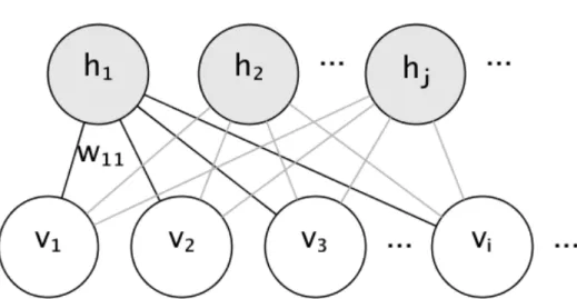
The graphical model of an RBM[2] is a fully-connectedbipartitegraph as in Fig. 3.3: The nodes are random variables whose states depend on the state of the other nodes they are connected to. The model is therefore parametrized by the weights of the connections, as well as one intercept (bias) term for each visible and hidden unit. The energy function measures the qual-ity of a joint assignment:

E(v,h) =X i X j wijvihj+ X i bivi+ X j cjhj. (3.18)

In the above formula, b and c are the intercept vectors for the visible and hidden layers, respectively. The joint probability of the model is defined in terms of the energy:

P(v,h) = e −E(v,h)

3.3.1 Bernoulli Restricted Boltzmann machines

In the Bernoulli RBM, all units are binary stochastic units. This means that the input data should either be binary, or real-valued between 0 and 1 signifying the probability that the visible unit would turn on or off[11]. This is a good model for character recognition, where the interest is on which pixels are active and which aren’t. For images of natural scenes it no longer fits because of background, depth and the tendency of neighbouring pixels to take the same values. In the Bernoulli RBM, both hidden units and visible units are not internally connected while the visible layer and the hidden layer are fully connected to each other. As a result, the conditional probabilities can be factorized as follows: P(v|h) =Y i P (vi|h), (3.20) P(h|v) = Y i P (hi|v), (3.21) and P (vi = 1|h) = sigmoid X j wijhj +bi ! , (3.22) P (hi = 1|v) = sigmoid X i wijvi+cj ! . (3.23)

3.3.2 Maximum Likelihood Learning

RBM is an unsupervised learning method, The learning goal is to max-imize the logarithmic probability given by

logP(v) = logX

h

e−E(v,h)−logX

x,y

To implement gradient descent in minimization, we need the following deriva-tives of the log-likelihood function:

∂logP(v) ∂wij = −X h P(h|v)∂E(v,h) ∂wij +X h,v p(v,h)∂E(v,h) ∂wij = P(hi = 1|v)vj − X v P(v)P(hi = 1|v)vj, (3.25) ∂logP(v) ∂bj = −X h P(h|v)∂E(v,h) ∂bj +X h,v p(v,h)∂E(v,h) ∂bj = vj − X v P(v)vj, (3.26) ∂logP(v) ∂ci = −X h P(h|v)∂E(v,h) ∂ci +X h,v p(v,h)∂E(v,h) ∂ci = P(hi = 1|v)− X v P(v)P(hi = 1|v), (3.27)

where we have applied

∂E(v,h) ∂wij =hivj, (3.28) ∂E(v,h) ∂bj =vj, (3.29) ∂E(v,h) ∂cj =hj. (3.30) 3.3.3 Contrastive divergence

Due to the summation over a large number of input data in the gra-dient evaluation, all common training algorithms for RBMs approximate the log-likelihood gradient given some data and perform gradient ascent on these

approximations. Obtaining unbiased estimates of log-likelihood gradient using MCMC methods typically requires many sampling steps. However, recently it was shown that estimates obtained after running the chain for just a few steps can be sufficient for model training. This leads to contrastive divergence (CD) learning, which has become a standard way to train RBMs.

The idea of k-step contrastive divergence learning (CD-k) is quite sim-ple: Instead of approximating the second term in the log-likelihood gradient by a sample from the RBM-distribution (which would require to run a Markov chain until the stationary distribution is reached), a Gibbs chain is run for only k steps (and usually k= 1). As a result,

∂logP v(0) ∂wij ≈ −X h P hv(0)∂E v (0)_,h ∂wij +X h p hv(k)∂E v (k)_,h ∂wij = P hi = 1 v(0)v(0)_j −P hi = 1 v(k)v(_jk), (3.31) ∂logP v(0) ∂bj ≈ −X h P hv(0)∂E v (0)_,h ∂bj +X h p hv(k)∂E v (k)_,h ∂bj = v_j(0)−v_j(k), (3.32) ∂logP v(0) ∂cj ≈ −X h P hv(0)∂E v (0)_,h ∂cj +X h p hv(k)∂E v (k)_,h ∂cj = P hi = 1 v(0)−P hi = 1 v(k). (3.33)

3.4

Deep auto-encoder

The idea of deep auto-encoder was proposed in the seminal paper by Hinton[11], where stacked RBMs were used to encode image data. The struc-ture of a stacked RBM is shown in Fig.3.4. Instead of a single layer of hidden

units, multiple layers of feature detectors with different dimensions are acti-vated by sigmoid functions except for the top layer. After learning one layer of feature detectors, their activities are treated as input for learning a second layer of features. The first layer of feature detectors then become the visible units for learning the next RBM. This layer-by-layer learning can be repeated as many time as desired. In Hinton’s work, the visible units of every RBM had real-valued activities, which were in the range [0,1] for logistic units. While training higher level RBMs, the visible units were set to the activation proba-bilities of the hidden units in the previous RBM, but the hidden units of every RBM except the top one had stochastic binary values. The hidden units of the top RBM have stochastic real-valued states drawn from a unit variance Gaussian whose mean was determined by the input from that RBM’s logistic visible units. This type of deep auto-encoder had been tested on MNIST data and facial images[11].

It is difficult to optimize the weights in nonlinear auto-encoders that contains multiple layers[11]. With large initial weights, auto-encoders typically find poor local minima; with small initial weights, the gradients in the early layers are tiny, making it infeasible to train auto-encoders with many hidden layers. If the initial weights are close to a good solution, gradient descent in backpropagation works well. This optimal initialization is obtained through a layer-by-layer unsupervised learning algorithm and each layer is trained as in an individual RBM. This has proved to be a very efficient and effective ’pre-training’ stage.

In Pankaj’s work[14], it was proved and demonstrated that stacked RBM is intimately related to one of the most important and successful tech-niques in theoretical physics, renormalization group (RG), which is an iterative coarse-graining scheme that allows for the extraction of relevant features as a physical system is examined at different length scales. In their work, an exact mapping between variational RG and deep learning architectures based on RBM was constructed and implemented on the ferromagnetic Ising model. In this report, we followed their work and demonstrated the power of deep auto-encoders using nearest-neighbor Ising Model in two-dimensional square lattice.

Figure 3.1: The architecture of a feed-forward artificial neural network with a single hidden layer. The output probabilities of each neuron in the hidden layer are served as inputs for the output layer. (This figure was clipped from online course materials at coursera.com)

Figure 3.2: The architecture of CNN. The input is a colored picture with a 2d grid of pixels. Two convolution+pooling layers are used to convert pixels into 1d input data for the fully connected layer as in the feed-forward neural network[1].

Figure 3.3: The architecture of restricted Boltzmann machine: the hidden units on the top are connected to the visible units at the bottom. There is no internal connections between units in the hidden layer[2].

(a)

(b)

Figure 3.4: The architectures of auto-encoders[3]: (a) Auto-encoder with a sin-gle hidden layer and the sigmoid activation function. (b) Deep auto-encoder with stacked RBMs as encoding layers and the decoding layers have the re-versed dimensions.

Chapter 4

Data-preparation and model specification

In this chapter, we describe the procedure of data generation, process-ing and visualization. Then we lay out the structures of our models and specify the choices of parameters.

4.1

Ferromagnetic Ising model

4.1.1 Data

The data for ferromagnetic Ising model was generated by metropolis Markov chain Monte Carlo sampling described in Chapter 2. For training and testing purposes in supervised learning, we generated Ising spin configurations taking binary values{1,−1}from 50 different temperatures (kBT) evenly

dis-tributed from 1.0 to 3.6 (We set the Ising coupling constant J = 1.0). From each temperature we generated 2500 data points for training sets and 250 data points for test sets. In order to obtain the critical temperatureT∗ in the ther-modynamic limit, we trained our model on datasets of different system size

L = 10,20,30,40,60 and the critical temperature for each system size was identified.

phase (PM) as 1 and the low temperature ferromagnetic phase (FM) as 0. The features in the datasets includeL×L spins labeled as (ix −1)×L+iy, ix =

1,2, . . . , L;iy = 1,2, . . . , L. (Table.4.1)

For RBMs and the deep autoencoder in unsupervised learning, we gen-erated Ising spin configurations taking binary values {0,1} from system size

L = 40 with temperature kBT = 2.451 (close to the critical temperature).

Our sample size was 50000 and we applied a train-test split with test size proportion equal to 0.2 in the whole dataset.

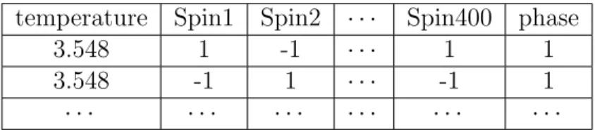
temperature Spin1 Spin2 · · · Spin400 phase

3.548 1 -1 · · · 1 1

3.548 -1 1 · · · -1 1

· · · ·

Table 4.1: Sample data frame for L= 20 Ising model.

4.1.2 Model

For supervised learning, we used a feed-forward ANN with one hidden layer containing 400 sigmoid hidden units to classify the binary phases in the Ising model. The optimizer was chosen to be stochastic gradient descent (SGD) with batch size equal to 100 the number of epochs equal to 10. Our learning rate was 0.001 and the weight decay was equal to 1e−6.

For unsupervised learning, we implemented a deep auto-encoder with stacked RBMs as illustrated in Fig.3.4. The visible layer of the first RBM

contains 40×40 = 1600 binary units and the first hidden layer contains 400 units taking real values within [0,1) serving as the visible units for the second RBM. The third layer contain 100 units and our encoding model was topped with 25 hidden units. Our encoding model was trained layer by layer with contrastive divergence for 200 epochs and momentum 0.5 using batch size 100 on 40000 total training samples.

4.2

Ising gauge model

4.2.1 Data

The data for Ising gauge model was generated by metropolis Markov chain Monte Carlo sampling described in Chapter 2 with both spin flips and gauge updates where we chose s = 0.75. For training and testing purposes in supervised learning, we generated Ising gauge spin configurations taking binary values {1,−1}from system size L= 4,8,12,16,20,24,28 with T close to 0 and ∞ respectively (Again we set the Ising coupling constant J = 1.0). From each temperature we generated 25000 data points for training sets and 2500 data points for test sets.

For each data point, we labeled the high temperature deconfined phase as 0 and the low temperature confined phase as 1. The features in the datasets include 2×L×L spins defined on the links. We divided our spins into two sublattices: spins on x links and spins on y links, Spins on x links are labeled as (ix−1)×L+iy, ix= 1,2, . . . , L;iy = 1,2, . . . , L, while spins on y links are

As input for CNN model, one needs to reshape the data into (2, L, L) such that two-dimensional feature detectors can be applied to scan the lattice. 4.2.2 Model

The model we implemented includes a convolutional layer first followed by a ReLu layer, and then followed by a 2-d max pooling layer. The convo-lutional layer applies 64 2×2 filters to the configuration on each sublattice and the pooled features were then flattened into 1-d arrays. The outcome was served as input data into a fully connected layer with 64 units and a softmax output layer. To prevent overfitting, a dropout regularization ratep= 0.1 was added to the fully connected layer.

Chapter 5

Results

5.1

Feed-forward ANN on ferromagnetic Ising model

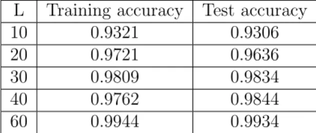
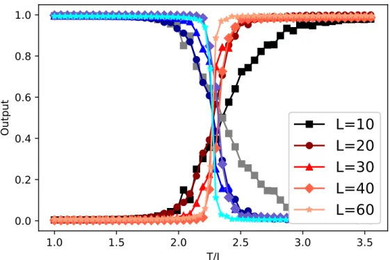
As mentioned in the previous chapter, our feed-forward ANN was trained on 50 different temperatures with 2500 data points per temperature. The pre-dicted probabilities for the test set were averaged over 250 data points per temperature and shown in Fig.5.1. The transition temperature from FM to PM (i.e. critical temperature) was decided by the intersection between the output layer and the base modelp= 0.5. We noticed that with the increase of system size L, the output probability drops (increases) more sharply around the critical temperature. This is due to O(L2) increase in the number of in-put features. The training and test accuracy for different L’s are listed in Table.5.1.

L Training accuracy Test accuracy

10 0.9321 0.9306

20 0.9721 0.9636

30 0.9809 0.9834

40 0.9762 0.9844

60 0.9944 0.9934

1.0 1.5 2.0 2.5 3.0 3.5 T/J 0.0 0.2 0.4 0.6 0.8 1.0 O ut pu t

L=10

L=20

L=30

L=40

L=60

Figure 5.1: The output layer of our trained feed-forward neural network model averaged over a test set as a function of T/J for the square-lattice ferromagnetic Ising model of sizeL= 10,20,30,40,60.

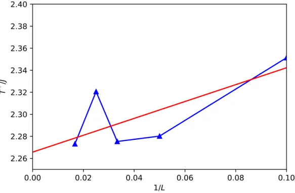
From the predicted critical temperatureTc forL= 10,20,30,40,60, we

could estimate the critical temperatureT∗ in the thermodynamic limitL=∞

by finite size scaling. The procedure was carried out first by a linear regression

y = w∗x+b with the least square fitting, where the response variable y is

Tc and the input variable is 1/L, and then by extracting the intercept b as

an estimate of T∗. The T-1/L plot and the fitted line are shown in Fig. 5.2 and the scaling analysis estimates T∗/J ≈ 2.266, which is pretty close to the

theoretical value T∗/J = 2/ln(1 +√2)≈2.269. 0.00 0.02 0.04 0.06 0.08 0.10 1/L 2.26 2.28 2.30 2.32 2.34 2.36 2.38 2.40 T * /J

Figure 5.2: The plot for finite size scaling of the critical temperatureTc/J ∼

1/L. The red line is the fitted result.

5.2

Deep auto-encoder on ferromagnetic Ising model

As mentioned in Chapter 3, our deep auto-encoder consists of stacked RBMs with 400-100-25 hidden units. We performed a layer-by-layer pretrain-ing on the encodpretrain-ing layers. After the weights and biases for each RBM were obtained, the model was ’unfolded’ to produce encoder and decoder networks.

(a) (b)

Figure 5.3: Visualization of effective receptive fields for (a) 100 spins in the middle layer, (b) 25 spins in the top layer. Each 40 by 40 pixel image depicts the effective receptive field of one of the spins in the hidden units.

Since the decoded layer has reversed dimensions between visible units and hidden units compared to the encoded layer, the weight matrix for the de-coded layer is the transpose of the one in the ende-coded layer and the biases in the visible units and the hidden units are switched between the two layers. With this initialization of parameters, one can perform back-propagation in the global fine-tuning stage with a much better starting point compared to random initialization.

To better understand the unsupervised learning results in the pretrain-ing stage, the effective receptive fields[14] are defined as follows: We denote the effective receptive field matrix of layerl byr(l) _{and the number of spins in} layer l by n(l)_{, with the visible layer corresponding to l = 0. Each column in}

r(l) _{is a vector that encodes the receptive field of a single spin in hidden layer}

l. It can be computed by convoluting the weight matrices W(l) _{encoding the} weights wij between the spins in layers l−1 and l. To compute r(l) first we

setr(1) _=W(1) _{and used the recursion relationship r}(l) _=r(l−1)_W(l) _{for l >1.} Thus the effective field is a measure of how much that hidden spin influences the spins in the visible layer and a way to visualize which spins in the visible layer that coupled to that hidden spin. In Fig.5.3, we plotted the density of the effective receptive fields by color maps for the middle layer with 100 spins and for the top layer with 25 spins. It can be observed that the receptive fields are localized in the visible spins and get larger as one moves up the in the encoded layers. As pointed out in Pankaj’s work[14], this is consistent with what is ex-pected from the successive application of block renormalization group method in statistical mechanics, indicating that the architecture of stacked RBMs is implementing a coarse-graining scheme similar to block spin renormalization. Moreover, the size of the blocks coupling to each hidden unit in a layer are of approximately the same size. In conclusion, this local block spin structure emerging from the pretraining process strongly suggests that stacked RBMs are self-organizing to implement block-spin renormalization.

In the back-propagation fine-tuning stage, we compared the training result with that of random initialization in Fig.5.4, where the logarithmic likelihood loss as a function of epochs was monitored for randomly initialized and pre-trained models. By observation, one is able to find that the deep auto-encoder makes rapid progress after pre-training but little progress without

0 50 100 150 200 # of passes over data

0.52 0.54 0.56 0.58 0.60 0.62 0.64 0.66 0.68 0.70 Lo ss pe r da ta p oi nt

Figure 5.4: Loss per data point in the fine tuning stage as a function of number of epochs trained for the deep auto-encoder. The green curve corresponds to random initialization in the model parameter. The blue curve is initialized with pre-trained model parameters.

pre-training. This is consistent with the result from Hinton’s work[11].

With the fine-tuned parameters, our model can be applied to recon-struct the Ising spin configurations in the test dataset. In Fig.5.5, we gener-ated the reconstructed spin configurations by Bernoulli sampling based on the predicted probabilities for each spin on the lattice sites.

5.3

CNN on Ising gauge model

We employed CNN to train the Ising gauge models with system size

Figure 5.5: Reconstructed spin configurations (lower) compared to the corre-sponding raw configurations (upper).

fromT = 0 states with an accuracy of 100% on both training and test datasets except for L = 4, in which 95.54% and 95.15% accuracy was achieved on the training and test set respectively. To examine the origin of the discriminative power of CNN, one can check whether it discerns T = 0 states from T = ∞

states by the presence and absence of satisfied local constraints, i.e. whether the 4-spin state on a plaquette q is such that Q

iσ z

i = 1. We constructed

new test sets with modified low temperature states: applying transformations where a spin is flipped every m = 2 and m = 4 plaquettes (Fig. 5.6). Such transformations were proved not to destroy the topological order of theT = 0 state where the extended closed loop structure was preserved, but they change the local constraints of the original Ising lattice gauge theory. Our model for

L = 20 showed that the prediction accuracy drops to 50% and 82.77% for

of local constraints instead of the extended loop structure.

Figure 5.6: The spin flip transformations on the links inx direction every m

plaquettes forL= 20, wherem= 2 for the upper row andm = 4 for the lower row. From left to right: spin configurations before the transformation, spin configurations after the transformation, spins changed under the transforma-tion indicated by the white spots.

Chapter 6

Conclusion and discussion

In this report, we presented our study on the deep neural network application in the Ising type models on the square lattice. Our results mostly reproduced the work by Juan[7] and Pankaj[14] and showed the discriminative and encoding power of deep neural networks.

In the application of feed-forward ANN to the ferromagnetic Ising model, one can understand the training of the network through a simple toy model involving a hidden layer of only three analytically ’trained’ perceptrons[7], representing the possible combinations of high- and low-temperature magnetic states exclusively on the basis of their magnetization, which plays the role of the order parameter in the model. The fully connected ANN relies on the order parameter in the classification task. It has also been shown that the power of feed-forward ANNs lies in their ability to generalize to different lat-tice structures[7].

In the application of CNN to Ising gauge model, we have shown that deep learning methods can encode basic information about unconventional phases and we demonstrated the power of CNN in local constraints detection even though the model itself does not have an order parameter. In Juan[7]’s

work, a toy model using streamlined version of the original CNN was con-structed to detect satisfied local constraints and estimate the cross over tem-perature. The analytical model they presented indicated that neural networks have the potential to represent ground state wavefunctions of unconventional topological states.

In the application of deep auto-encoders, we illustrated by Ising model that the mechanism behind stacked RBMs is similar to the iterative coarse-graining procedure in RG. We also demonstrated the influence of pre-training in reconstructing the spin configurations in analogy to the image and the hand-written digit reconstruction problems.

Overall, our study suggests a prospectively enormous applications of deep learning algorithms in solving notoriously difficult many-body problems in physics. As in all other areas of ”big data”, we anticipate the rapid adoption of machine learning techniques as a basic research tool in statistical mechanics.

Appendix 1

Sample code

We present sample codes in Python here for both supervised and un-supervised learning.

1.1

Keras implementation of feed-forward ANN in

fer-romagnetic Ising model

# c o d i n g : u t f−8 # In [ 1 ] :

import pandas a s pd import numpy a s np import k e r a s

from k e r a s . models import S e q u e n t i a l from k e r a s . l a y e r s import Dense

from k e r a s . o p t i m i z e r s import SGD from k e r a s import r e g u l a r i z e r s import m a t p l o t l i b . p y p l o t a s p l t g e t i p y t h o n ( ) . magic ( u ’ m a t p l o t l i b i n l i n e ’ ) # In [ 2 ] : def r e a d d a t a ( L ) : ””” : t y p e L : i n t ( s y s t e m s i z e )

: r t y p e t r a i n , t e s t : pd . d a t a f r a m e ( w i t h p h a s e s l a b e l e d ) ””” t r a i n f i l e n a m e= ’ c o n f i g u r a t i o n ’+s t r( L )+ ’ . c s v ’ t e s t f i l e n a m e= ’ t e s t ’+s t r( L )+ ’ . c s v ’ columns =[ ’ t e m p e r a t u r e ’ ] + [ ’ S p i n ’+s t r( i ) f o r i in xrange( 1 , L∗L+1) ] t r a i n=pd . r e a d c s v ( ’ I s i n g d a t a / ’+ ’ L ’+s t r( L )+ ’ / ’+ t r a i n f i l e n a m e , names=columns ) t e s t=pd . r e a d c s v ( ’ I s i n g d a t a / ’+ ’ L ’+s t r( L )+ ’ / ’+ t e s t f i l e n a m e , names=columns ) # d e c i d e c r i t i c a l t e m p e r a t u r e f i l e n a m e= ’ Cv ’+s t r( L )+ ’ . c s v ’ s p e c i f i c h e a t=pd . r e a d c s v ( ’ I s i n g d a t a / ’+ ’ L ’+s t r( L )+ ’ / ’+f i l e n a m e , names =[ ’ t e m p e r a t u r e ’ , ’ Cv ’ ] ) Tc=s p e c i f i c h e a t [ ’ t e m p e r a t u r e ’ ] [ np . argmax ( s p e c i f i c h e a t [ ’ Cv ’ ] ) ] # add p h a s e column t r a i n [ ’FM ’ ] = [i n t(T<=Tc ) f o r T in t r a i n [ ’ t e m p e r a t u r e ’ ] ] t e s t [ ’FM ’ ] = [i n t(T<=Tc ) f o r T in t e s t [ ’ t e m p e r a t u r e ’ ] ] t r a i n [ ’PM’ ] = [i n t(T>Tc ) f o r T in t r a i n [ ’ t e m p e r a t u r e ’ ] ] t e s t [ ’PM’ ] = [i n t(T>Tc ) f o r T in t e s t [ ’ t e m p e r a t u r e ’ ] ] return t r a i n , t e s t # In [ 3 ] : t r a i n , t e s t=r e a d d a t a ( 2 0 ) # In [ 2 5 ] : t r a i n . t a i l ( )

# In [ 4 ] :

def d a t a p r o c e s s ( t r a i n , t e s t ) :

”””

: t y p e t r a i n , t e s t : pd . d a t a f r a m e ( w i t h p h a s e s l a b e l e d ) : r t y p e trX , trY , teX , teY

”””

# s h u f f l e

t r a i n=t r a i n . sample ( f r a c =1) . r e s e t i n d e x ( drop=True ) trX , trY = t r a i n . drop ( [ ’FM ’ , ’PM’ , ’ t e m p e r a t u r e ’ ] , a x i s

=1) , np . a r r a y ( t r a i n [ [ ’FM ’ , ’PM’ ] ] )

teX , teY = t e s t . drop ( [ ’FM ’ , ’PM’ , ’ t e m p e r a t u r e ’ ] , a x i s =1) , np . a r r a y ( t e s t [ [ ’FM ’ , ’PM’ ] ] )

return trX , trY , teX , teY

# In [ 5 ] :

trX , trY , teX , teY=d a t a p r o c e s s ( t r a i n , t e s t )

# In [ 1 8 ] : def c r e a t e m o d e l ( h i d d e n u n i t s =3 , lamb = 0 . 0 5 , l r = 0 . 0 0 1 ) : c l a s s i f i e r =S e q u e n t i a l ( ) c l a s s i f i e r . add ( Dense ( o u t p u t d i m=h i d d e n u n i t s , i n i t = ’ u n i f o r m ’ , k e r n e l r e g u l a r i z e r=r e g u l a r i z e r s . l 2 ( lamb ) , a c t i v a t i o n= ’ s i g m o i d ’ , i n p u t d i m=trX . s h a p e [ 1 ] ) ) c l a s s i f i e r . add ( Dense ( o u t p u t d i m =1 , i n i t = ’ u n i f o r m ’ , k e r n e l r e g u l a r i z e r=r e g u l a r i z e r s . l 2 ( lamb ) , a c t i v a t i o n= ’ s i g m o i d ’ ) )

sgd = SGD( l r = 0 . 0 0 1 , decay=1e−6)#, momentum=0.9 , n e s t e r o v=True ) c l a s s i f i e r .compile( o p t i m i z e r= ’ adam ’ , l o s s= ’ b i n a r y c r o s s e n t r o p y ’ , m e t r i c s =[ ’ a c c u r a c y ’ ] ) return c l a s s i f i e r # In [ 1 9 ] : c l a s s i f i e r =c r e a t e m o d e l ( h i d d e n u n i t s =400) # In [ 2 0 ] : c l a s s i f i e r . f i t ( np . a r r a y ( trX ) , np . argmax ( trY , a x i s =1) , b a t c h s i z e =100 , n b e p o c h =5 , v e r b o s e =1) # In [ 2 1 ] : y p r e d= c l a s s i f i e r . p r e d i c t ( np . a r r a y ( teX ) ) # In [ 2 2 ] :

np . mean ( ( y p r e d>0 . 5 ) [ : , 0 ] = = np . argmax ( teY , a x i s =1) )

# In [ 2 3 ] : Temperatures=np . a r r a y (sorted(l i s t(s e t( t e s t [ ’ t e m p e r a t u r e ’ ] ) ) ) ) P r e d a v g s = [ ] num T=Temperatures . s h a p e [ 0 ] n u m t e s t=len( t e s t [ ’ t e m p e r a t u r e ’ ] ) b a t c h=n u m t e s t /num T

f o r i in xrange( num T ) : s t a r t=b a t c h∗i end=s t a r t+b a t c h b a t c h p r e d i c t i o n=y p r e d [ s t a r t : end ] P r e d a v g s . append ( np . mean ( b a t c h p r e d i c t i o n , a x i s =0) ) P r e d a v g s=np . a r r a y ( P r e d a v g s ) # In [ 2 4 ] : import m a t p l o t l i b . p y p l o t a s p l t g e t i p y t h o n ( ) . magic ( u ’ m a t p l o t l i b i n l i n e ’ ) p l t . p l o t ( Temperatures , P r e d a v g s [ : , 0 ] , ’ bo ’ , Temperatures , P r e d a v g s [ : , 0 ] , ’ b−’ , Temperatures , 1−P r e d a v g s [ : , 0 ] , ’ r o ’ , Temperatures , 1−P r e d a v g s [ : , 0 ] , ’ r−’ ) # In [ ] :

1.2

Keras implementation of CNN in Ising gauge model

# c o d i n g : u t f−8 # In [ 1 ] : import pandas a s pd import numpy a s np # In [ 2 ] : def r e a d d a t a ( L ) : ””” : t y p e L : i n t ( s y s t e m s i z e ) : r t y p e t r a i n , t e s t : pd . d a t a f r a m e ( w i t h p h a s e s l a b e l e d )

””” t r a i n f i l e n a m e= ’ c o n f i g u r a t i o n ’+s t r( L )+ ’ . c s v ’ t e s t f i l e n a m e= ’ t e s t ’+s t r( L )+ ’ . c s v ’ columns =[ ’ t e m p e r a t u r e ’ ] + [ ’ S p i n ’+s t r( i ) f o r i in xrange( 1 , 2∗L∗L+1) ] t r a i n=pd . r e a d c s v ( ’ I s i n g g a u g e d a t a / ’+ ’ L ’+s t r( L )+ ’ / ’ +t r a i n f i l e n a m e , names=columns ) t e s t=pd . r e a d c s v ( ’ I s i n g g a u g e d a t a / ’+ ’ L ’+s t r( L )+ ’ / ’+ t e s t f i l e n a m e , names=columns ) # S e p a r a t e T=0 and T=i n f Tc=2.

# add p h a s e column (T=0: 1 , T=i n f : 0 )

t r a i n [ ’ p h a s e ’ ] = [i n t(T<=Tc ) f o r T in t r a i n [ ’ t e m p e r a t u r e ’ ] ] t e s t [ ’ p h a s e ’ ] = [i n t(T<=Tc ) f o r T in t e s t [ ’ t e m p e r a t u r e ’ ] ] return t r a i n , t e s t # In [ 3 ] : L=8 t r a i n , t e s t=r e a d d a t a ( L ) # In [ 4 ] : t r a i n . head ( ) # In [ 5 ] : def d a t a p r o c e s s ( t r a i n , s h u f f l e=True ) : ”””

: t y p e t r a i n , t e s t : pd . d a t a f r a m e ( w i t h p h a s e s l a b e l e d ) : r t y p e trX , trY , teX , teY

””” # s h u f f l e i f s h u f f l e : t r a i n=t r a i n . sample ( f r a c =1) . r e s e t i n d e x ( drop=True ) # s e p a r a t e A, B s u b l a t t i c e s t r a i n A=t r a i n [ [ ’ S p i n ’+s t r( i ) f o r i in xrange( 1 , L∗L+1) ] ] . a s m a t r i x ( ) t r a i n B=t r a i n [ [ ’ S p i n ’+s t r( i ) f o r i in xrange( L∗L+1 ,2∗ L∗L+1) ] ] . a s m a t r i x ( ) trX=np . z e r o s ( ( t r a i n A . s h a p e [ 0 ] , L , L , 2 ) ) trX [ : , : , : , 0 ] = np . r e s h a p e ( t r a i n A , ( t r a i n A . s h a p e [ 0 ] , L , L ) ) trX [ : , : , : , 1 ] = np . r e s h a p e ( t r a i n B , ( t r a i n B . s h a p e [ 0 ] , L , L ) ) trY = t r a i n [ ’ p h a s e ’ ] return trX , trY # In [ 6 ] : trX , trY=d a t a p r o c e s s ( t r a i n ) teX , teY=d a t a p r o c e s s ( t e s t ) # ∗∗c h e c k p l a q u e t t e∗∗ # In [ 7 ] : def p l a q u e t t e ( l i n k s ) : p l a q u e t t e = np . z e r o s ( ( l i n k s . s h a p e [ 0 ] , L , L ) )

f o r i in xrange( L ) : f o r j in xrange( L ) : p l a q u e t t e [ : , i , j ]= l i n k s [ : , i , j , 0 ]∗l i n k s [ : , i , j , 1 ] ∗l i n k s [ : , ( i +1)%L , j , 1 ]∗l i n k s [ : , i , ( j +1)%L , 0 ] return p l a q u e t t e # In [ 8 ] : p l a q=p l a q u e t t e ( trX ) p l a q # In [ 9 ] : # I m p o r t i n g t h e Keras l i b r a r i e s and p a c k a g e s

from k e r a s . models import S e q u e n t i a l from k e r a s . l a y e r s import Conv2D

from k e r a s . l a y e r s import MaxPooling2D from k e r a s . l a y e r s import F l a t t e n

from k e r a s . l a y e r s import Dense from k e r a s . l a y e r s import Dropout from k e r a s . o p t i m i z e r s import Adam

# In [ 1 0 ] : # I n i t i a l i s i n g t h e CNN c l a s s i f i e r = S e q u e n t i a l ( ) # S t e p 1 − C o n v o l u t i o n c l a s s i f i e r . add ( Conv2D ( 6 4 , ( 2 , 2 ) , i n p u t s h a p e = ( L , L , 2 ) , a c t i v a t i o n = ’ r e l u ’ ) ) # S t e p 2 − P o o l i n g

c l a s s i f i e r . add ( MaxPooling2D ( p o o l s i z e = ( 2 , 2 ) ) ) # S t e p 3 − F l a t t e n i n g c l a s s i f i e r . add ( F l a t t e n ( ) ) # S t e p 4 − F u l l c o n n e c t i o n c l a s s i f i e r . add ( Dense ( u n i t s = 6 4 , a c t i v a t i o n = ’ r e l u ’ ) ) # drop o u t c l a s s i f i e r . add ( Dropout ( p = 0 . 1 ) ) c l a s s i f i e r . add ( Dense ( u n i t s = 1 , a c t i v a t i o n = ’ s i g m o i d ’ ) ) # C o m p i l i n g t h e CNN adam=Adam( l r = 0 . 0 0 0 1 ) c l a s s i f i e r .compile( o p t i m i z e r = adam , l o s s = ’ b i n a r y c r o s s e n t r o p y ’ , m e t r i c s = [ ’ a c c u r a c y ’ ] ) # In [ 1 1 ] : c l a s s i f i e r . f i t ( trX , trY , b a t c h s i z e =100 , n b e p o c h =25 , v e r b o s e =0) # In [ 1 2 ] : t r y p r e d= c l a s s i f i e r . p r e d i c t ( trX ) t e y p r e d= c l a s s i f i e r . p r e d i c t ( teX ) # In [ 1 3 ] : np . mean ( ( t r y p r e d >0 . 5 ) [ : , 0 ] = = trY ) # In [ 1 4 ] :

t e y p r e d . s h a p e # In [ 1 5 ] : np . mean ( ( t e y p r e d>0 . 5 ) [ : , 0 ] = = teY ) # ∗∗p r e d i c t c r o s s−o v e r t e m p e r a t u r e on f i n i t e t e m p e r a t u r e d a t a∗ ∗: # In [ 1 6 ] : def r e a d f i n i t e ( L ) : f i l e n a m e= ’ t e s t f i n i t e T ’+s t r( L )+ ’ . c s v ’ columns =[ ’ b e t a ’ ] + [ ’ S p i n ’+s t r( i ) f o r i in xrange( 1 , 2∗ L∗L+1) ] d a t a=pd . r e a d c s v ( ’ I s i n g g a u g e d a t a / ’+ ’ L ’+s t r( L )+ ’ / ’+ f i l e n a m e , names=columns ) return d a t a # In [ 1 7 ] : def d a t a p r o c e s s f i n i t e ( t e s t ) : ””” : t y p e t r a i n , t e s t : pd . d a t a f r a m e ( w i t h p h a s e s l a b e l e d ) : r t y p e trX , trY , teX , teY

””” # s e p a r a t e A, B s u b l a t t i c e s t e s t A=t e s t [ [ ’ S p i n ’+s t r( i ) f o r i in xrange( 1 , L∗L+1) ] ] . a s m a t r i x ( ) t e s t B=t e s t [ [ ’ S p i n ’+s t r( i ) f o r i in xrange( L∗L+1 ,2∗L∗ L+1) ] ] . a s m a t r i x ( ) teX=np . z e r o s ( ( t e s t A . s h a p e [ 0 ] , L , L , 2 ) ) teX [ : , : , : , 0 ] = np . r e s h a p e ( t e st A , ( t e s t A . s h a p e [ 0 ] , L , L )

) teX [ : , : , : , 1 ] = np . r e s h a p e ( t e s t B , ( t e s t B . s h a p e [ 0 ] , L , L ) ) return teX # In [ 1 8 ] : t e s t f i n i t e =r e a d f i n i t e ( L ) teX=d a t a p r o c e s s f i n i t e ( t e s t f i n i t e ) # In [ 1 9 ] : y p r e d= c l a s s i f i e r . p r e d i c t ( teX ) # In [ 2 0 ] : y p r e d =( y p r e d >0 . 5 ) # In [ 2 1 ] : B e t a s=np . a r r a y (sorted(l i s t(s e t( t e s t f i n i t e [ ’ b e t a ’ ] ) ) ) ) P r e d a v g s = [ ] num T=B e t a s . s h a p e [ 0 ] n u m t e s t=len( t e s t f i n i t e [ ’ b e t a ’ ] ) b a t c h=n u m t e s t /num T f o r i in xrange( num T ) : s t a r t=b a t c h∗i end=s t a r t+b a t c h b a t c h p r e d i c t i o n=y p r e d [ s t a r t : end ] P r e d a v g s . append ( np . mean ( b a t c h p r e d i c t i o n , a x i s =0) )

P r e d a v g s=np . a r r a y ( P r e d a v g s ) # In [ 2 2 ] : import m a t p l o t l i b . p y p l o t a s p l t g e t i p y t h o n ( ) . magic ( u ’ m a t p l o t l i b i n l i n e ’ ) p l t . p l o t ( Betas , P r e d a v g s [ : , 0 ] , ’ bo ’ , Betas , P r e d a v g s [ : , 0 ] , ’ b−’ , Betas , 1−P r e d a v g s [ : , 0 ] , ’ r o ’ , Betas , 1−P r e d a v g s [ : , 0 ] , ’ r−’ ) # In [ 2 3 ] : teX . s h a p e # In [ 2 4 ] : b a t c h # In [ ] :

Bibliography

[6] Louis-Fran ¸cois Arsenault, Alejandro Lopez-Bezanilla, O. Anatole von Lilienfeld, and Andrew J. Millis. Machine learning for many-body physics: The case of the anderson impurity model. Phys. Rev. B, 90:155136, Oct 2014.

[7] Juan Carrasquilla and Roger G. Melko. Machine learning phases of matter. Nat Phys, 13(5):431–434, May 2017. Letter.

[8] Wen Xiao Gang. Quantum field theory of many-body systems: from the origin of sound to an origin of light and electrons. Oxford University Press, Oxford, 2007.

[9] Luca M. Ghiringhelli, Jan Vybiral, Sergey V. Levchenko, Claudia Draxl, and Matthias Scheffler. Big data of materials science: Critical role of the descriptor. Phys. Rev. Lett., 114:105503, Mar 2015.

[10] Ian Goodfellow, Yoshua Bengio, and Aaron Courville. Deep Learning.

MIT press, page 1, 2016.

[11] G. E. Hinton and R. R. Salakhutdinov. Reducing the dimensionality of data with neural networks. Science, 313(5786):504–507, 2006.

[12] Sergei V. Kalinin, Bobby G. Sumpter, and Richard K. Archibald. Big-deep-smart data in imaging for guiding materials design. Nat Mater, 14(10):973–980, Oct 2015. Progress Article.

[13] Aaron Gilad Kusne, Tieren Gao, Apurva Mehta, Liqin Ke, Manh Cuong Nguyen, Kai-Ming Ho, Vladimir Antropov, Cai-Zhuang Wang, Matthew J. Kramer, Christian Long, and Ichiro Takeuchi. On-the-fly machine-learning for high-throughput experiments: search for rare-earth-free permanent magnets. Sci. Rep., 4:6367, Sep 2014.

[14] Pankaj Mehta and David J. Schwab. An exact mapping between the Variational Renormalization Group and Deep Learning. arXiv, pages 1–7, oct 2014.

[15] Anders W. Sandvik. Computational studies of quantum spin systems.