Working Paper Series
Bootstrap-Based Improvements for Inference with Clustered Errors A. Colin Cameron University of California, Davis Douglas Miller University of California, Davis Jonah B. Gelbach Department of Economics, University of Maryland and College of Law, Florida State University July 14, 2006 Paper # 06-21 Microeconometrics researchers have increasingly realized the essential need to account for any within-group dependence in estimating standard errors of regression parameter estimates. The typical preferred solution is to calculate cluster-robust or sandwich standard errors that permit quite general heteroskedasticity and within-cluster error correlation, but presume that the number of clusters is large. In applications with few (5-30) clusters, standard asymptotic tests can over-reject considerably. We investigate more accurate inference using cluster bootstrap-t procedures that provide asymptotic refinement. These procedures are evaluated using Monte Carlos, including the much-cited differences-in-differences example of Bertrand, Mullainathan and Duflo (2004). In situations where standard methods lead to rejection rates in excess of ten percent (or more) for tests of nominal size 0.05, our methods can reduce this to five percent. In principle a pairs cluster bootstrap should work well, but in practice a Wild cluster bootstrap performs better. Department of Economics One Shields Avenue Davis, CA 95616 (530)752-0741 http://www.econ.ucdavis.edu/working_search.cfm
Bootstrap-Based Improvements for Inference with
Clustered Errors
A.Colin Cameron, Jonah B. Gelbachyand Douglas L. Millerz
June 14, 2006
Abstract
Microeconometrics researchers have increasingly realized the essen-tial need to account for any within-group dependence in estimating standard errors of regression parameter estimates. The typical pre-ferred solution is to calculate clustrobust or sandwich standard rors that permit quite general heteroskedasticity and within-cluster er-ror correlation, but presume that the number of clusters is large. In ap-plications with few (5-30) clusters, standard asymptotic tests can over-reject considerably. We investigate more accurate inference using clus-ter bootstrap-t procedures that provide asymptotic re…nement. These procedures are evaluated using Monte Carlos, including the much-cited di¤erences-in-di¤erences example of Bertrand, Mullainathan and Du‡o (2004). In situations where standard methods lead to rejection rates in excess of ten percent (or more) for tests of nominal size0:05, our methods can reduce this to …ve percent. In principle a pairs cluster bootstrap should work well, but in practice a Wild cluster bootstrap performs better.
Keywords: clustered errors; random e¤ects; cluster robust; sand-wich; bootstrap; bootstrap-t; clustered bootstrap; pairs bootstrap; wild bootstrap.
JEL Classi…cation: C15, C12, C21.
Department of Economics, University of California - Davis.
yDepartment of Economics, University of Maryland and College of Law, Florida State
University.
1
Introduction
Microeconometrics researchers have increasingly realized the essential need to account for any within-group dependence in estimating standard errors of regression parameter estimates. A leading example involves using ordinary least squares (OLS) and U.S. household survey data to estimate the e¤ects of changes in state policies on wages or labor supply. The policy regressor is perfectly correlated (invariant) within state and, even after control for many additional regressors, the error likely will be correlated within states given that states are thought of as distinct labor markets.
In such settings the default OLS standard errors that ignore such cluster-ing can greatly underestimate the true OLS standard errors, as emphasized by Moulton (1986, 1990).
A common correction is to compute cluster-robust standard errors that generalize the White (1980) heteroskedastic-consistent estimate of OLS stan-dard errors to the clustered setting. This permits both error heteroskedas-ticity and quite ‡exible error correlation within cluster, unlike a much more restrictive random e¤ects or error components model. In econometrics this adjustment was proposed by White (1984) and Arellano (1987), and it is im-plemented in STATA, for example, using the cluster option. In the statistics literature these are called sandwich standard errors, proposed by Liang and Zeger (1986) for generalized estimating equations, and they are implemented in SAS, for example, within the GENMOD procedure. A recent brief survey is given in Wooldridge (2003).
Not all empirical studies use appropriate corrections for clustering. In particular, for …xed e¤ects panel models the errors are usually correlated even after control for …xed e¤ects, yet many studies either provide no control for serial correlation or erroneously cluster at too …ne a level. Kezdi (2004) demonstrated the usefulness of cluster robust standard errors in this setting and contrasted these with other standard errors based on stronger distribu-tional assumptions. Bertrand, Du‡o, and Mullainathan (2004), henceforth BDM (2004), focused on implications for di¤erence-in-di¤erence (DID) stud-ies using data on individuals across states and years. Then the regressor of interest is an indicator variable that is highly correlated within cluster (state) so there is great need to correct standard errors for clustering. The clustering should be on state, rather than on state-year.
A practical limitation of inference with cluster-robust standard errors is that the asymptotic justi…cation assumes that the number of clusters goes to in…nity. Yet in some applications there may be few clusters. For example, this happens if clustering is on region and there are few regions. With a small number of clusters the cluster-robust standard errors are downwards biased. Bias corrections have been proposed in the statistics literature; see Kauermann and Carroll (2001), Mancl and DeRouen (2001), and Bell and McCa¤rey (2002). But even after appropriate bias correction, with few clusters the usual Wald statistics for hypothesis testing with asymp-totic standard normal or chi-square critical values over-reject. BDM (2004) demonstrate through a Monte Carlo experiment that the Wald test based on (unadjusted) cluster-robust standard errors over-rejects if standard nor-mal critical values are used. Donald and Lang (2004) also demonstrate this and propose, for DID studies with policy invariant within state, an alter-native two-step GLS estimator that leads to T-distributed Wald tests in some special circumstances. Angrist and Lavy (2002) in an applied study …nd that bias adjustment of cluster-robust standard errors can make quite a di¤erence.
In this paper we investigate whether bootstrapping to obtain asymptotic re…nement leads to improved inference for OLS estimation with cluster-robust standard errors when there are few clusters. We focus on cluster bootstrap-t procedures that are generalizations of those proposed for regres-sion with heteroskedastic errors in the nonclustered case. Previous studies have also investigated the performance of some cluster bootstraps, an early simulation study being that by Sherman and le Cressie (1997). But there have been relatively few such studies, and each study focuses on one partic-ular bootstrap method.
Several features of our bootstraps are worth emphasizing. First, the bootstraps involve resampling entire clusters. Second, our goal is to use variants of the bootstrap that provide asymptotic re…nement, whereas most econometric applications use the bootstrap only to obtain consistent esti-mates of standard errors. Third, we consider several di¤erent cluster re-sampling schemes: pairs bootstrap, residuals bootstrap and wild bootstrap. Fourth, we consider examples with as few as …ve clusters, as it is not un-usual in a clustered setting to have so few clusters yet still have parameter estimates su¢ ciently precise that coe¢ cients may be statistically signi…cant
at conventional signi…cance levels. Fifth, we evaluate our bootstrap proce-dures in a number of settings including examples of others that were used to demonstrate the de…ciencies of standard cluster-robust methods.
The paper is organized as follows. Section 2 provides a summary of standard asymptotic methods of inference for OLS with clustered data, and presents small-sample corrections to cluster-robust standard errors that have been recently proposed in the statistics literature. Section 3 presents various possible bootstraps for clustered data, with additional details relegated to an Appendix. Sections 4 to 6 present, respectively, a Monte Carlo experiment using generated data, a Monte Carlo experiment using data from BDM (2004), and an application using data from Gruber and Poterba (1994).
The primary contribution of this paper is to o¤er methods for more accurate cluster-robust inference. These methods are fairly simple to imple-ment and matter substantively in both our Monte Carlo experiimple-ments and our replications.
A second important contribution of this paper is to o¤er a careful and precise description of the various bootstraps a researcher might perform, and the similarities and di¤erences between our proposed methods and several commonly-applied methods. Our primary motivation for presenting this description is to be precise about our methods. However, it also o¤ers empiricists a clearer understanding of the menu of bootstrap choices and their consequences.
2
Cluster-Robust Inference
Before considering the bootstrap we present results on inference with clus-tered errors.
2.1 OLS with Clustered Errors
The model we consider is one withGclusters (subscripted byg), and withNg
observations (subscripted by i) within each cluster. Errors are independent across clusters but correlated within clusters. The model can be written at various levels of aggregation as
yig =x0ig +uig; i= 1; :::; Ng,g= 1; :::; G; yg =Xg +ug; g= 1; :::; G;
y =X +u;
where isk 1,xig isk 1,Xg isNg k,XisN k,N =PgNg,yig and
uig are scalar,yg andug areNg 1 vectors andy andu areN 1vectors.
Interest lies in inference for the OLS estimator
b = XG g=1 XNg i=1xigx 0 ig 1 XG g=1 XNg i=1xigyig (2) = XG g=1X 0 gXg 1 XG g=1X 0 gyg = (X0X) 1X0y:
Under the assumptions that data are independent over g but errors are correlated within cluster, with E[ug] =0, E[ugug0] = g, and E[ugu0h] =0
for cluster h6=g, we have b a N[ , V[b]] where V[b] = (X0X) 1 XG
g=1Xg gX
0
g (X0X) 1: (3)
This di¤ers from and is usually larger than the specialization
V[b] = 2u(X0X) 1 (4)
that is based on the assumption of iid errors and leads to thedefault OLS variance estimatewhen 2u is estimated bys2=ub0ub=(N k). In the case where the primary source of clustering is due to group-level common shocks, a useful approximation is that for thejthregressor the default OLS variance
estimate should be in‡ated by thevariance in‡ation multiplier
j '1 + xj u(Ng 1); (5)
where xj is the within cluster correlation of xj, u is the within cluster
error correlation, and Ng is the average cluster size. This result is exact
if cluster sizes are identical, all regressors are invariant within cluster (so
xj = 1) and the error follows a random e¤ects model, de…ned below. In practice it provides a useful guide in a range of settings.1 As one example, if there are 81 observations per cluster, the regressor is invariant within 1Kloek (1981) provides the special case. Scott and Holt (1982) and Greenwald (1983)
give more general results for unbalanced clustering and within-cluster regressor and error correlation that varies across clusters. Similar variance in‡ation arises in survey design, for example two-stage sampling, and in that literature the multiplier is called the design e¤ect.
cluster, and u = 0:10, then default OLS standard errors should be in‡ated byp1 + 0:1 80 =p9 = 3.
Clearly it can be important to control for clustering, a point emphasized by Moulton (1986, 1990) and more recently by BDM (2004). The underesti-mation bias is increasing in (1) cluster size; (2) within-cluster correlation of the regressor; and (3) within-cluster correlation of the error. The challenge for inference is that g is unknown.
2.2 Moulton-type Standard Errors
One approach is to model g to depend on unknown parameters, say g = g( ), and then use estimate bg = g(b). The random e¤ects (RE)
modelspeci…es
uig = g+"ig, g iid[0; 2],"ig iid [0; 2"]: (6)
Then V[uig] = 2u = 2"+ 2, Cov[uig; ujg] = 2, and u = Cor[uig; uig0] =
2=( 2
"+ 2)is called the error intraclass correlation coe¢ cient. This model
yields cluster error covariance matrix g = 2"INg +
2e
Nge0Ng, where eNg is anNg 1 vector of ones, and we use variance estimate
b VRE[b] = (X0X) 1 XG g=1XgbgX 0 g (X0X) 1; (7) where bg=b2"INg +b 2e Nge0Ng, and b 2
" and b2 are consistent estimates for
2
"and 2. We call the resulting standard errorsMoulton-type standard
errors.
2.3 Cluster-Robust Variance Estimates
The RE model places restrictions of homoskedasticity and equicorrelation within cluster. A less parametrically restrictive approach is to use the
cluster-robust variance estimator (CRVE)
b VCR[b] = (X0X) 1 XG g=1Xgeugue 0 gX0g (X0X) 1; (8)
which is consistent ifplimG 1PGg=1Xgeugueg0X0g= plimG 1 PG
g=1Xg gX0g.
Standard errors based onVbCR[b]are calledclustrobust standard
The CRVE controls for both error heteroskedasticity across clusters and quite general correlation and heteroskedasticity within cluster, at the ex-pense of requiring that the number of clusters G! 1. It is implemented for many STATA regression commands using the cluster option (which uses
e
ug =pcubg wherec= GG1NN k1 ' GG1 with largeN), and is used in SAS in
the GENMOD procedure (which uses eug =ubg).
The CRVE estimate is an immediate extension of theheteroskedastic consistent covariance matrix estimator (HCCME) of White (1980) for nonclustered data, i.e. in the special caseNg = 1. Many of the methods
we consider below can be viewed as extensions to the clustered case to proposed adaptations of the nonclustered HCCME case.
2.4 Unbiased Cluster-Robust Variance Estimates
A weakness of the standard CRVE with ueg = bug is that it is biased, since
E[ubgub0g] 6= g = E[ugu0g]. The bias depends on the form of g but will
usually be downwards.2 Several corrected residuals ueg for (8) have been
proposed. The simplest, already mentioned, is to useueg= p
G=(G 1)ubg.
Kauermann and Carroll (2001) and Bell and McCa¤rey (2002) use
e
ug = [INg Hgg]
1=2
b
ug; (9)
where Hgg = Xg(X0X) 1X0g. This transformed residual leads to unbiased
CRVE in (8) in the special case that g = 2I, though in simulations the
authors …nd the correction works quite well even if g 6= 2I.3 Bell and
McCa¤rey (2002) also use
e ug = r G 1 G [INg Hgg] 1ub g: (10)
Then VbCR[b] in (8) with ueg calculated using (10) can be shown to equal
the jackknife estimate of the variance of the OLS estimator.4 This jackknife 2
For example, Kezdi (2004) usesueg=ubgand …nds in his simulations that withG= 10
the donwards bias is between9and16percent.
3
These papers, and that by Bell, McCa¤rey and Botts (2001), also propose corrections for the more general case that g6= 2I, provided g has a known parameterization, and
for extension to generalized linear models.
4The jackknife drops in turn each observation, here a cluster, computes the
leave-one-out estimate b(g), g= 1; :::; G, and then uses variance estimate G 1
G P
correction does not make an assumption about g, and leads to
downwards-biased CRVE if in fact g = 2I. Angrist and Lavy (2002) apply the
cor-rection (9) in an application withG= 30to40 and …nd that the correction increases cluster-robust standard errors by between 10 and 50 percent.
Similar corrections have been well-studied for the HCCME in the non-clustered case. The correction (9) generalizes the HC2 measure of MacK-innon and White (1985) that sets ueg = (1 hgg) 1=2 where hgg is the gth
diagonal entry ofX(X0X) 1X0 and is called the leverage measure in the lit-erature on in‡uential data points.5 The correction (10) generalizes the HC3
measure (jackknife) of MacKinnon and White (1985). Chesher and Jewitt (1987) obtain HCCME bias results under the more general assumption that errors are heteroskedastic rather than iid, and show that the performance of various HCCME corrections depends crucially on the leverage measures, with greater problems the larger is the maximum leverage. Chesher and Austin (1991) emphasize that di¤erent design matricesXcan lead to di¤er-ent assessmdi¤er-ents of HCCMEs, a result that can be expected to carry over to the clustered case.
We refer to the residual correction (10) as the CR3 variance estima-tor, since it is a cluster extension of the HC3 procedure. An additional complication in the clustered setting is that for some con…gurations of the regressor design matrixINg Hggneed not be full rank, leading to problems in implementing these corrections.
2.5 Cluster-Robust Wald Tests
We consider two-sided Wald tests of H0 : 1 = 01 against Ha : 1 6= 01
where 1 is a scalar component of .6 We use theWald test statistic
w= b1 0 1 sb 1 ; (11)
Applied to the OLS estimator, some algebra yields jackknife estimate of variance (8) where
e ug = p (G 1)=G[INg Hgg] 1 b
ug. This is a multiple of the related measure proposed
by Mancl and DeRouen (2001) in the more general setting of GEE.
5The motivation is that b u=Mu, whereM=I X(X0X) 1 X0, so that for E[uu0] = 2 I, E[ubbu0] =M 2IM= 2M. It follows that E[ub2g] = 2Mgg, so E[(M 1=2 gg ubg)2] = 2. 6The generalization to single hypothesisc0 r= 0wherecis ak 1vector is trivial.
where sb
1 is the square root of the appropriate diagonal entry in
b
VCR[b].
This "t" test statistic is asymptotically normal underH0, and we rejectH0
at signi…cance level ifjwj> z =2, wherez =2 is a standard normal critical value. Often = 0:05, in which casez =2 = 1:960.
Under standard assumptions the Wald test is of correct size as the num-ber of clustersG! 1. The problem we focus on in this paper is that with few clusters the asymptotic normal critical values can provide a poor ap-proximation to the correct, …nite-Gcritical values forw, even if an unbiased variance matrix estimator is used in calculatingsb.
Small sample results are not possible even if the (clustered) errors are normally distributed. Some intuition can be gained, however, by considering balanced clusters (Ng = NG) with all regressors invariant within cluster
(xig =xg)and errorsuig that are iidN[0; 2]. OLS estimation at either the
individual level or the aggregate level will lead to the same OLS estimator. But the estimate of 2 di¤ers, leading to t-tests with quite di¤erent degrees of freedom.
Using individual-level data,yig =x0g +uig, the Wald test statistic using
default OLS standard errors is distributed T(N k), since the errors are iid normal. Suppose we instead use aggregated data,yg=x0g +ug. Then the
OLS estimator equals that from the individual-level regression, as clusters are balanced. Since ug are iidN[0; 2=NG]the Wald statistic using default
OLS standard errors is T(G k) distributed. The very large loss of degrees of freedom is due to aggregation leading to a di¤erent estimate of 2: here
s2 = (G k) 1Pgbu2g rather thans2 = (N k) 1PgPibu2ig .
Now suppose we instead use the CRVE in forming the Wald statistic for OLS estimation with individual-level data. This robust Wald statistic is no longer T distributed, even if the errors are iid normal. Some algebra yields
b VCR[b] = (Pgxgx0g) 1( P gub 2 gxgx0g)( P gxgx0g) 1, where ubg = Ng1 P iubig.
This is a more variable variance estimator than that used with aggregated data and default OLS standard errors, which can be expanded as Vb[b] = (Pgxgx0g) 1( P gs2xgx0g)( P gxgx0g) 1 with s2 = (G k) 1 P hub 2 h. Given
this more variable estimate of sb
1, the Wald statistic using cluster robust standard errors will have fatter tails than those of a T(G k) distribu-tion. For more detailed discussion of a related result for the HCCME, see Kauermann and Carroll (2001).7
In practice, as a small sample correction some programs use a T distri-bution to form critical values and p-values. STATA uses the T(G 1) dis-tribution, which the preceding example suggests is better than the standard normal, but may still not be conservative enough to avoid over-rejection. Bell and McCa¤rey (2002) and Pan and Wall (2002) propose instead using a T distribution with degrees of freedom determined using an approximation method due to Satterthwaite (1941).
Rather than use OLS, Donald and Lang (2004) propose an alternative two-step estimator that leads to a Wald test that in some special cases is T(G k1)distributed wherek1 is the number of regressors that are invariant
within cluster and oftenk1= 2 (the intercept and the clustered regressor of
interest).
We instead continue to use the standard OLS estimator with CRVE, and bootstrap to obtain bootstrap critical values that provide an asymptotic re…nement and may work better than other inference methods for OLS when there are few clusters.
3
Cluster Bootstraps
Bootstrap methods generate a number of pseudo-samples from the original sample, for each pseudo-sample calculate the statistic of interest, and use the distribution of this statistic across pseudo-samples to infer the distribution of the original sample statistic. This is very similar to a Monte Carlo sim-ulation, except the pseudo-samples are generated using fewer distributional assumptions.8
There is no single bootstrap as there are di¤erent statistics that we may be interested in, di¤erent ways to form pseudo-samples, and even for a given statistic and resampling method there are di¤erent ways to use results for statistical inference.
We provide considerable discussion here and in the appendix because in later sections we use a range of bootstrap methods that may be unfamiliar
standard deviation 2 to 3 times that for default standard errors. He does not consider the implications for Wald tests.
8The bootstrap was introduced by Efron (1979). Standard book treatments are Hall
(1992), Efron and Tibsharani (1993), and Davison and Hinkley (1997). In econometrics see Horowitz (2001), MacKinnon (2002), and the texts by Davidson and MacKinnon (2004) and Cameron and Trivedi (2005).
to applied microeconometricians. The statistic considered is the Wald test statisticw de…ned in (11), for two-sided test ofH0 : 1 = 01 against Ha :
16= 01.
The data are clustered into G independent groups, so the resampling method should be one that assumes independence across clusters but pre-serves within cluster features such as correlation.
3.1 Pairs Cluster Bootstrap-T
The obvious method is to resample the clusters with replacement from the original sample f(y1;X1); :::;(yG;XG)g. The following procedure provides
a starting point.
Pairs Cluster Bootstrap-T Procedure
1. DoB iterations of this step. On the bth iteration:
(a) Form a sample of G clusters f(y1;X1); :::;(yG;XG)g by resam-pling with replacementGtimes from the original sample. (b) Calculate the Wald test statistic
wb = b1;b b1
sb
1;b
;
whereb1;bis obtained from OLS estimation using thebth pseudo-sample, its standard errorsb
1;bis estimated using the same cluster-robust method as used in calculating w, and b1 is the original sample OLS estimate.
2. Use the empirical distribution ofw1; :::; wBto determine critical values andp-values. Thus rejectH0 at level if and only if
w < w[ =2] or w > w[1 =2];
wherew[q] denotes theqth quantile of w1; :::; wB.9 9ForBrealizationsx1; :::; x
B, theqthquantilex[q]is the smallest value ofxsuch that a
proportionq ofx1; :::; xB are less than or equal tox[q]. More formally x[q] is the smallest
As an example, ifw= 2:10,w[:025]= 2:32 and w[:975]= 1:87 then we would not rejectH0 at signi…cance level = 0:05 since 2:10 does not fall
outside( 2:32;1:87). This is called a nonsymmetric test, as the critical values in the two tails di¤er. We could also do a symmetric two-tailed test, in which case in step 2 we would rejectH0 ifjwj>jw j[ ], wherejw j[q]
denotes theqth quantile ofjw
1j; :::;jwBj.
This resampling method is called a pairs cluster bootstrap because, unlike other methods presented below, the pair(y;X) is jointly resampled. Alternative names used in the literature include cluster bootstrap,case bootstrap,nonparametric bootstrap, andnonoverlapping block boot-strap. Because this resampling method views the original sample as the dgp (with 1 = b1), the pseudo-sample statistics wb are centered on this dgp valueb1.
The bootstrap-t procedure, proposed by Efron (1981) for con…dence intervals, is also called a percentile-t procedure, because the “t” test statisticwis bootstrapped, and a studentized bootstrap, since the Wald test statistic is a studentized statistic. The bootstrap-t procedure has ad-vantages that we now present.
3.2 Asymptotic Re…nement of Standard Bootstrap Methods
The bootstrap-t procedure was preceded by more obvious bootstrap proce-dures that bootstrap the parameter estimateb1, givingBestimatesb1;1; :::;b1;B, rather than the test statistic.
Thepercentile proceduresimply rejectsH0if the original sample
esti-mateb1 falls outside(b1;[ =2];b1;[1 =2])whereb1;[q]denotes theqthquantile
of(b1;1; :::;b1;B).
The bootstrap-se procedure uses these estimates to form the boot-strap estimate of standard error
sb 1;B = 1 B 1 B X b=1 (b1b b1)2 !1=2 ; (12) where b1 = B1 PBb=1b1b, uses sb
1;B to calculate the Wald test, so
wBSE = b1 0 1 sb 1;B ; (13)
and rejectsH0 at signi…cance level if and only if jwBSEj> z =2. Here the
bootstrap is used merely to obtain an estimate of the standard error ofb1, an advantage if this is di¢ cult to do using conventional methods.
The bootstrap-t, percentile and bootstrap-se procedures are all asymp-totically valid tests under standard modelling assumptions. In particular, a test at nominal (or desired) signi…cance level0:05 will have true size of 0.05 (and power of 1.00 against a …xed alternative) asG! 1.
But for small G all three procedures will have true size di¤erent from 0.05 as they rely on asymptotic approximation. Consider a test with nominal signi…cance level or nominal size . An asymptotic approximation yields an actual rejection rate ortrue size +O(G j=2), whereO(G j=2)means is of order G j=2 and G is the number of clusters. Then the true size goes to as G ! 1, provided j > 0. Larger j is preferred, however, as then convergence to is faster. A bootstrap providesasymptotic re…nement
if it leads to j larger than that for conventional (…rst-order) asymptotic methods.
Asymptotic re…nement is more likely to occur if the bootstrap is applied to an asymptotically pivotal statistic, meaning one with asymptotic distribution that does not depend on unknown parameters; see Appendix A.1 for a more complete discussion. The cluster-robust Wald statistic is asymptotically pivotal as it is standard normal (no unknown parameters), so the bootstrap-t procedure provides asymptotic re…nement. By contrast the percentile and bootstrap-se methods bootstrap the OLS estimator, which is not asymptotically pivotal as the asymptotic variance is dependent on unknown parameters.
The bootstrap-t procedure is not the only way to obtain an asymptotic re…nement. In particular, the bias-corrected accelerated (BCA) pro-cedure, de…ned in Appendix A.2, is a variation of the percentile method that leads to asymptotic re…nement of the same order as the percentile-t method.
3.3 Wild Cluster Bootstrap-T
For a regression model with additive error, resampling methods other than pairs cluster can be used. In particular, one can hold regressorsXconstant throughout the pseudo-samples, while resampling the residuals which can be then used to construct new values of the dependent variabley.
The obvious method is a residual cluster bootstrap that resamples with replacement from the original sample residual vectors to give residuals fub1; :::;buGg and hence pseudo-sample f(by1;X1); :::;(byG;Xg)g where byg = X0gb+ubg.
This resampling scheme has two weaknesses. First, it assumes that the regression error vectorsug are iid, whereas in Section 2 we were speci…cally
concerned that the variance matrix g will di¤er across clusters. Second, it
presumes a balanced data set where all clusters are the same size. The next bootstrap relaxes both these restrictions.
Wild Cluster Bootstrap-T Procedure
1. Obtain the OLS estimator b and the associated OLS residuals ubg,
g= 1; :::; G.
2. DoB iterations of this step. On the bth iteration:
(a) For each clusterg= 1; :::; G, formubg =ubgwith probability0:5or b
ug = ubg with probability0:5, and hence ybg =X0gb+bug. This
yields wild cluster bootstrap resamplef(yb1;X1); :::;(ybG;XG)g.
(b) Calculate the OLS estimate b1;b and its standard errorsb
1;b and given these form the Wald test statisticwb = (b1;b b1)=sb
1;b. 3. RejectH0 at level if and only if
w < w[ =2] or w > w[1 =2];
wherew[q] denotes theqth quantile of w1; :::; wB.
The wild bootstrap was proposed by Wu (1986) for regression in the nonclustered case. Its asymptotic validity and asymptotic re…nement were proven by Liu (1988) and Mammen (1993). Horowitz (1997, 2001) provides a Monte Carlo demonstrating good size properties. We use a version, called Rademacher weights, that o¤ers asymptotic re…nement ifbis symmetrically distributed, the case if errors are symmetric. If b is asymmetrically distrib-uted, our version is still asymptotically valid, but a di¤erent version provides asymptotic re…nement. Davidson and Flachaire (2001) provide theory and simulation to support using Rademacher weights even in the asymmetric
case. See Appendix Section A.3 for further discussion. Here we have ex-tended the wild bootstrap to a clustered setting. The only study to do so that we are aware of is the brief application by Brownstone and Valletta (2001).
Several authors, particularly Davidson and MacKinnon (1999), advocate use of bootstrap resampling methods that impose the null hypothesis. This is possible using both residual and Wild bootstraps. Thus we present results based on bootstraps that impose the null, in which case the bootstrap Wald statistics are centered on 01 rather than b1, and the residuals bootstrapped are those from the restricted OLS estimator e that imposes H0 : 1 = 01.
For details see Appendix A.2.
3.4 Bootstraps with Few Clusters
With few clusters the bootstrap resampling methods produce a distinctly …-nite number of possible pseudo-samples, so the bootstrap distributionw1; :::; wq
will not be smooth even for large B. Furthermore, in some pseudo-samples
b1 orsb
1 may be inestimable.
First, consider pairs cluster resampling. Each bootstrap resample con-tainsGclusters. Some of the original sample clusters will appear more than once, while others will not appear at all. For example, withG= 5we might obtain bootstrap resample f(y3;X3);(y5;X5);(y2;X2);(y3;X3);(y1;X1)g.
In general, this bootstrap has 2GG 11 possible unordered recombinations of the data; see Hall (1992, p.283). There are many possible combinations even when there are few clusters: 126combinations for G= 5 and 92;378 com-binations for G= 10. Nonetheless, implementation problems can arise. For example, if thekth regressor is binary and is always invariant within cluster (so always0 or always1for given g) then with few clusters some bootstrap resamples may have all clusters with thekthregressor taking only value0(or value1), so thatbkis inestimable. This issue does not arise when regressors and dependent variables take many di¤erent values, such as in the Section 4 Monte Carlos. But it does arise in our application to the BDM (2004) and Gruber and Poterba (1994) di¤erences-in-di¤erences example, because the regressors of interest in those cases are indicator variables.
Second, consider the wild cluster bootstrap. For each cluster there are two possible resample values, so withGclusters there are2Gpossible
recom-binations: 32combinations forG= 5and1;024combinations forG= 10. In general this is much less than for pairs cluster. However, a binary regressor invariant within cluster will not cause a problem as we are not resampling the regressors. And, as clear from Appendix A.2, the Wild bootstrap need not be restricted to a two-point distribution, though we do not pursue this.
3.5 Bootstrap Discussion
Clearly there are many ways to bootstrap when data are clustered. The stan-dard applied procedure is to use pairs cluster resampling and the bootstrap-se procedure which o¤ers no asymptotic re…nement.10 There are just a few
studies that we are aware of that consider asymptotic re…nement.
In the statistics literature, Sherman and le Cessie (1997) conduct sim-ulations for OLS with as few as ten clusters. For 90 percent con…dence intervals, they …nd that the pairs cluster bootstrap-t undercovers by con-siderably less than the percentile method which in turn is better than using conventional robust con…dence intervals based on cluster-robust standard errors. The bootstrap-t intervals are wider than the others, however, and occasionally have very large end-points. The authors also study logit mod-els, and they …nd occasionally that bootstrap resamples are inestimable due to all dependent variables taking value zero (or one).
Flynn and Peters (2004) consider cluster randomized trials where a pairs cluster bootstrap draws G clusters by separately resampling from the G=2
treatment clusters and the G=2 control clusters. For skewed data and few clusters they …nd that pairs cluster BCA con…dence intervals have consider-able undercoverage, even more than conventional robust con…dence intervals, though in their Monte Carlo design the robust intervals do remarkably well. The authors also consider a second-stage of resampling within each cluster, using a method for hierarchical data given in Davison and Hinkley (1997) that is applicable if the random e¤ects model (6) is assumed.
In the econometrics literature, BDM (2004) apply a pairs cluster boot-strap using the bootboot-strap-t procedure. BDM use default OLS standard er-rors, however, rather than cluster-robust standard erer-rors, in computing both the original data and the resampled data Wald statistics. Because of this 1 0Stata, for example, o¤ers this as an estimation option. Additionally it has a
clus-ter pairs bootstrap procedure that does provide BCA con…dence inclus-tervals in addition to bootstrap-se con…dence intervals, but these are rarely used.
their method will in general not yield tests of correct size. It can nonetheless lead to considerable size improvement compared to using default standard errors, since it controls for any inconsistent estimation of standard errors up to a constant scale factor. Speci…cally, if w is computed using a sb
1 and
wb is computed usinga sb
1
, for constanta >0 that does not vary across bootstrap samples, then we obtain the same rejection rate regardless of the value of a and asymptotic re…nement is obtained.11 For the BDM exam-ple the scale factor is data-dependent, however, and varies across bootstrap resamples. The authors …nd that their bootstrap does better than using default OLS standard errors and standard normal critical values, yet sur-prisingly does worse than using cluster robust standard errors with standard normal critical values.
The only study we know of that uses wild bootstraps in a clustered setting is the brief application by Brownstone and Valletta (2001).
3.6 Test Methods used in this Paper
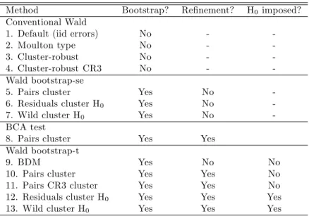
In the remainder of the paper we implement the Wald test using nine boot-strap procedures, as well as four non-bootboot-strap procedures. Table 1 provides a summary.
Our …rst four tests do not use the bootstrap and di¤er only in the method from section 2 used to calculate Vb[b]. They use, respectively, the default variance estimate (4), the Moulton-type estimate (7), the cluster-robust esti-mate (8), and the cluster-robust estiesti-mate with jackknife corrected residuals (10). Method 1 is invalid if there is clustering, method 2 is invalid unless the clustering follows a random e¤ects model, while methods 3 to 4 are asymptotically valid provided clusters are independent.
Methods 5 to 7 use the bootstrap-se procedure, with bootstrap standard error computed using (12) and Wald statistic using (13). We use three dif-ferent cluster bootstrap resampling methods, respectively, the pairs cluster bootstrap, the residual clusters bootstrap with H0 imposed, and the wild
bootstrap with H0 imposed. For details see Appendix A.2.3. Methods 5-7
do not provide asymptotic re…nement, and method 6 is valid only if cluster error vectors are iid.
1 1This fact follows since the cdf of a random variable is invariant to monotonic
Method 8 uses the BCA bootstrap with pairs cluster resampling, see Appendix A.2.2, to provide an asymptotic re…nement.
Methods 9 to 13 use the bootstrap-t procedure. The …rst three of these methods use pairs cluster resampling with di¤erent standard error estimates. Method 9 is the already discussed method of BDM that uses default stan-dard errors rather than CRVE stanstan-dard errors. Methods 10 and 11 use di¤erent variants of the CRVE de…ned in (8), respectively, the standard CRVE and the CR3 correction. In each case the same variance matrix esti-mation method is used for both the original sample and bootstrap resamples. Methods 12 and 13 use, respectively, residual and wild bootstraps, and both use the standard CRVE estimate and impose H0. Method 12 is valid only
if cluster error vectors are iid. For details see Appendix A.2.1.
The bootstrap-t and BCA procedures should set the number of bootstrap replications B so that (B + 1) is an integer. For an explanation see Davidson and MacKinnon (2004, p.164), for example. Additionally for low
B there will be nontrivial simulation error in the bootstrap. A common choice isB= 999, since 1,000 is an integer for common values of such as = 0:05.
4
Monte Carlo Simulations
To examine the …nite-sample properties of our methods we conducted sev-eral Monte Carlo exercises for dgp a linear model with intercept and single regressor. The error is clustered according to a random e¤ects model, with either constant correlation within cluster or departures from this induced by heteroskedasticity. This design is relevant to a cross-section study of in-dividuals with clustering at the state level, for example. The regressor and dependent variable are continuous and take distinct values across clusters and (usually) within clusters, so that even with few clusters it is unlikely that a pairs cluster bootstrap sample will be inestimable.
Then
yig = 0+ 1xig+uig; (14)
so = [ 0 1]0, with di¤erent generating processes for xig and uig used in subsequent subsections. Estimation is by OLS, as in (1). Since 1 = 1 in the dgp, we set 01 = 1 and the Wald test statistic isw= (b1 1)=sb
We performR replications, where each replication yields a new draw of data from the dgp, and leads to reject or nonrejection of H0 depending on
whether or not jwj > 1:96. In each replication there are G groups (g = 1; :::; G), with NG individuals(i= 1; :::; NG) in each group. We varied the
number of groups G from 5 to 30 and usually set NG = 30. The various
methods used down each column of Tables 2-4 are then applied to the same generated data. For bootstraps we usedB = 399bootstraps rather than the recommendedB = 999or higher. This lower value is …ne for a Monte Carlo exercise, since the bootstrap simulation error will cancel out across Monte Carlo replications.
We estimate the actual rejection rate a, by ba, the fraction of the R
replications for whichH0 is rejected. This is an estimate of the true size of
the test which should be0:05. With a …nite number of replicationsamay be di¤er from the true size due to simulation error. The simulation standard error is sba =
p
ba(1 ba)=(R 1). For R = 1000 replications, sba '0:007for ba= 0:05 and sba '0:009 for a = 0:10. We can reject that true size is the
desired0:05at the 95% signi…cance level when jba 0:05j>1:96 sba. With
R= 1000a value ofba= 0:07 will be statistically signi…cantly di¤erent from
0:05, while a value ofba= 0:06 will not.12
4.1 Simulations with Homoskedastic Clustered Errors
In the …rst simulation exercise both regressors and errors are correlated within group, with errors homoskedastic. Data were generated according to:
yig = 0+ 1xig+uig = 0+ 1(zg+zig) + ("g+"ig); (15)
withzg,zig, "g, and "ig each an independentN[0;1] draw, and 0 = 0and 1 = 1. Here the components zg and "g that are common to individuals
within a group induce within group correlation of both regressors and errors with x = 0:5 and u = 0:5. The simulation is based on R = 1000 Monte Carlo replications.
Our …rst results appear in Table 2. Each column gives results for the various number of groups(G= 5,10,15,20,25,30)and throughout NG=
30. The …rst entry is the estimated true size of the test, the proportion 1 2
Values of R higher than 1;000 would be better, but each entry in a table already requiresRB'400;000separate estimations.
of times the null hypothesis is rejected. The Monte Carlo standard error is given in parentheses. Each row presents a di¤erent method, detailed in section 3.6. For comparison, we also show the rejection rate that would hold if we used the asymptotic normal critical value of1:96, but the Wald statistic actually had a T distribution withG k=G 2degrees of freedom. This rejection rate is Pr[jTj > 1:96jT TG 2], though recall from section
2.5 that even with normal errors the …nite distribution of the various Wald statistics is unknown.
We begin with conventional (nonbootstrap) Wald tests using di¤erent estimators of standard errors. The default OLS standard errors that as-sume iid errors do poorly here, with rejection rates given in row 1 of0:43to
0:50 that are much higher than0:05.13 This illustrates the need to correct
standard errors for clustering. The Moulton-type estimate for standard er-rors should work well here since it this takes advantage of correct knowledge of the dgp. The rejection rates in row 2 are considerably higher than0:05, especially for low G, though are similar to those expected if the Wald test statistic is actually T(G 2)distributed (see the bottom row). The cluster-robust standard errors lead to rejection rates much better than those using default standard errors, though still over-reject with rejection rates that are
0:01 to 0:06 greater than those using Moulton-type standard errors. The CR3 correction to cluster-robust standard errors leads to larger standard errors and to rejection rates that from row 4 are much closer to0:05, though still signi…cantly di¤erent from0:05.
We then consider using the bootstrap to compute standard errors. The pairs cluster bootstrap-se method yields rejection rates in row 5 that are very similar to the cluster-robust method, except for G = 5. The residual cluster bootstrap-se method leads to rejection rates in row 6 that are close to0:05. From row 7, the wild cluster bootstrap-se method under-rejects for
G 10, and rejects at level close to0:05 forG >10. The closeness to 0:05
of the latter two bootstrap methods is surprising given that they do not o¤er an asymptotic re…nement.
The BCA bootstrap with pairs cluster resampling should provide an 1 3These rejections rates are consistent with theory. The dgp is a classic
bal-anced two-way random e¤ect error, so (5) applies yielding standard error in‡ation
p
1 + (30 1)0:5 0:5 =p8:25 = 2:87. Using the underestimated standard errors leads to a Wald statistic with actual asymptotic size equal toPr[jzj>1:96=2:87]'0:50. This underestimation depends on group size rather than number of groups.
asymptotic re…nement, yet from row 8 it has rejection rates similar to those using CR standard errors (row 3), aside from small improvement forG= 5
and G= 10where the rejection rates are nonetheless still in excess of 0:10. The remainder of the Table use the theoretically preferred bootstrap-t procedure with various resampling methods. Even though it uses default standard errors, the BDM bootstrap (row 9) does better than using CR standard errors and is a great improvement compared to not bootstrapping (row 1). The pairs cluster bootstrap-t has rejection rates in row 10 of 0:08
that are much closer to 0:05 than tests without bootstrap, though they are still signi…cantly di¤erent from 0:05. The CR3 correction makes little di¤erence. Apparently while it leads to considerable decrease in the value of the Wald statistic (see the di¤erence in rejection rates between rows 3 and 4), comparable decreases occur in the bootstrap resamples leading to similar rejection rates. Both the residual cluster bootstrap-t and wild cluster bootstrap-t rejection rates are not statistically di¤erent from0:05 (with the exception of the residual bootstrap with G= 5).
In summary, Table 2 demonstrates that all the bootstrap-t methods are an improvement on the usual cluster-robust method with standard normal critical values; the BCA method provides no improvement; and the residual cluster bootstrap-se also performs well.
4.2 Simulations with Heteroskedastic Clustered Errors
The second simulation brings in the additional complication of heteroskedas-tic errors. Then the Moulton-type correction and the residual bootstrap are no longer valid theoretically.
We generated data according to the process:
yig = + xig+uig = + (zg+zig) + ("g+"ig); (16)
with zg, zig, "g and "g again independent N[0;1] draws, but now "ig
N[0;9 (zg+zig)2]. The dgp sets = 1 and = 1. Here x = 0:5 again,
while the error is heteroskedastic both within and across clusters and has correlation coe¢ cient less than the Table 2 case of0:5.
Results appear in Table 3. Default OLS standard errors again do poorly, with rejection rates hovering around 0:30, though these results are better than those in Table 2 due to the lower error correlation in the present design.
The Moulton-type correction breaks down given the heteroskedasticity, as expected, with rejection rates in row 2 of 0:17 0:26. The cluster-robust methods do a little better than in the preceding table, but in rows 3 and 4 still generally exceed0:05.
The residual cluster bootstrap-se method now breaks down due to het-eroskedasticity, with rejection rates in row 6 in excess of 0:15. The pairs cluster bootstrap-se and wild cluster bootstrap-se methods (rows 5 and 7) perform similarly to Table 2.
The BCA bootstrap again has rejection rates in row 8 similar to those using CR standard errors (row 3), aside from small improvement forG= 5
and G= 10.
The results for the bootstrap-t methods in rows 9 to 13 are similar to those in Table 2. The incorrect BDM bootstrap-t (row 9) has similar high rejection rates to those in Table 2, aside from marked deterioration forG= 5. The remaining bootstrap-t methods all yield rejection rates less than0:08, with the residual cluster bootstrap-t and wild cluster bootstrap-t doing best. The good performance of the residual cluster bootstrap-t is surprising given that errors are heteroskedastic across clusters.
In summary, the Table 3 results for inference with heteroskedastic clus-tered errors are similar to those for homoskedastic clusclus-tered errors except that, as expected, the Moulton-type correction and residual cluster bootstrap-se methods now perform very poorly. The bootstrap-t methods are an im-provement on the usual cluster-robust method with standard normal critical values, while the BCA method provides no improvement.
4.3 Alternative Critical Values, Cluster Sizes and Regressor Design
We perform a third set of Monte Carlo experiments to examine how the di¤erent estimators perform under varying assumptions. These simulations are presented in Table 4 with each simulation based onG= 10groups.
Column 1 of Table 4 provides a baseline against which the other results are compared. It uses the same dgp as that of Table 2, though the simu-lations begin from a di¤erent seed so that actual rejection rates di¤er from theG= 10column in Table 2 due to simulation variability.
Tables 2 and 3 used asymptotic normal critical values in performing the Wald test using methods 1 to 7. In Table 4 column 2 we instead use critical
values from a T distribution with 8 degrees of freedom, an ad hoc …nite sample correction, so that we reject H0 if jwj > 2:306 rather than jwj > 1:960. Then the Moulton-type estimator and the CR3 correction lead to rejection rates not statistically signi…cant from0:05. The CR standard errors and pairs cluster bootstrap-se still lead to over-rejection, though by not as much. And the residual cluster bootstrap-se and wild cluster bootstrap-se, which seem to do very well when asymptotic normal critical values are used, now lead to great under-rejection.
In columns 3 to 5 of Table 4 we consider alternative cluster sizes of, respectively, 2, 10 and 100 observations, whereas Tables 2 and 3 always usedNG= 30observations per cluster. For method 1, the e¤ect of ignoring
clustering altogether increases greatly with cluster size, as predicted by (5). Once clustering is accounted for, by any of methods 2-13, rejection rates do not vary signi…cantly with cluster size.
In column 6 of Table 3 we examine the performance of the various testing methods when there are there are three additional regressors, each with no clustering component, and we continue to test the …rst regressor. The four regressors are scaled down by a factor of 1/2, so that the sum of their variances will equal the variance of the single regressor used in the dgp of column 1. The only signi…cant change in rejection rates is an increase in the already high rejection rate for method 1 which neglects clustering.
All preceding regression designs set the intraclass correlation x of the regressor of interest to be0:5. In column 7 we increase x to x = 1 (cluster-invariant regressor with xig = zg) and in column 8 we decrease x = 0 in
column 8 (iid regressor withxig =zig). In both cases the regressor is scaled
up byp2to keep V[xig]unchanged.
With cluster-invariant regressor (column 7) the failure to control for clustering is magni…ed and the row 1 rejection rate is largest than that in the benchmark column 1, as expected; the other nonbootstrap methods that attempt to control for clustering also have higher rejection rates. For bootstrap-se and bootstrap-t there is little change in rejection rates, except that for reasons unknown the pairs cluster bootstrap (both bootstrap-se and bootstrap-t) now has rejection rates not statistically signi…cantly di¤erent from0:05.
With iid regressor (column 8) and the current random e¤ects dgp for the errors formula (5) predicts that the default OLS standard errors are
consistent and the rejection rate in row 1 is close to0:05. The Moulton-type and CR estimators also have rejection rates much closer to0:05. The various bootstrap procedures lead to rejection rates that are all within0:03of those in column 1, with no obvious pattern.
Finally, in column 9 we change the dgp to examine an unbalanced setting, so that one half of the clusters are small (with group sizeNG= 10) and half
of the clusters are large (with group size NG = 50). The residual cluster
bootstrap requires equal cluster sizes, so it cannot be used in this design. The remaining methods yield results qualitatively similar to those in column 1, with the main change being that the standard CRVE leads to much larger over-rejection in row 3.14
In summary, all the bootstrap-t methods are an improvement on the usual cluster-robust method with standard normal critical values; the BCA method provides no improvement; and the residual cluster bootstrap-se also performs well.
Table 4 indicates that when non-bootstrap methods are used to control for clustering, it is better to use critical values from a T distribution than from a standard normal, results vary little with cluster size, and control-ling for clustering is more di¢ cult as the regressors become more highly correlated within cluster. Rejection rates for bootstrap-t methods varied little across the various designs, except that the pairs cluster and pairs CR3 bootstrap-t methods performed better when regressors are cluster invariant. The remaining conclusions are similar to those from Tables 2 and 3. Again the bootstrap-t methods are an improvement on the usual cluster-robust method, while the BCA method provides no improvement. And again for the bootstrap-t with pairs cluster resampling there is no advantage to making …nite sample corrections to the CRVE.
1 4
For the pairs cluster bootstrap we select with replacement ten clusters, so that with unbalanced cluster sizes the number of observations in each bootstrap pseudo-sample will generally di¤er fromN. By contrast the wild cluster bootstrap pseudo-samples will all be of sizeN.
5
Bertrand, Du‡o and Mullainathan (2004)
Sim-ulations
To enable a more practically familiar application of our methods, we now consider the di¤erences-in-di¤erences setup explored in Bertrand, Du‡o, and Mullainathan (2004).15
The data set is of U.S. states over time. The dependent variable is the state-by-year average log wage level (after partialling out certain individual characteristics). For such a variable, the error term within cluster is serially correlated, even if state and year …xed e¤ects are included as regressors. By contrast the random e¤ects model implies equicorrelation for the error term within cluster. The regressor of interest is a state policy dummy variable that is binary, making it more likely that with few clusters a pairs cluster bootstrap sample will be inestimable.
The original data is CPS data on many individuals over time and states. Most of the BDM (2004) study uses a smaller data set that aggregates individual observations to the state-year level. We begin with these data, which have the advantage of being balanced and relatively small, before moving to the individual data.
5.1 Aggregated State-year Data
Using our choice of subscripts, the igth observation is for the ith year in the gth state. There are …fty states and twenty-one years, so G = 50 and
NG= 21. The model estimated is
yig = g+ i+ 1Iig+uig;
whereyig is a year-state measure of excess earnings (after control for age and
education), the regressors are state dummies, year dummies, and a policy change indicatorIig.16
1 5We extracted individual-level data from the relevant CPS data sets and, when
appro-priate, aggregated these data using the method presented in BDM (2004). This gave data similar to that in BDM (2004). We thank these authors for sharing some of their data with us, enabling this comparison.
1 6We retain our notation for consistency with the rest of our discussion. However, more
obvious subscripts for this problem are ifor individual, s for state andt for year. The underlying model isyist= s+ t+xist0 + Ist+uist, whereyistis individual log-earnings
If a policy change occurs in stategat timei , thenIig = 0fori < i and
Iig = 1 fori i . BDM’s experiments randomly assign a policy change to
occur in half the states, and when it does occur it occurs somewhere between the sixth and …fteenth year. Since policy changes happen only once and are not reversed, the regressorIig will be highly correlated overifor state g. In
each simulation a di¤erent draw ofGstates with replacement is made from the original50 states.
The Wald statistic studied is w=b1=sb
1. BDM investigate size proper-ties by letting the policy change be a “placebo” regressor that has no e¤ect on yig. So for two-sided tests of H0 : 1 = 0 againstHa: 1 6= 0 at
signi…-cance level0:05we should rejectH0 in …ve percent of the simulations. They
also investigate the power against the alternative powerHa : 1 = 0:02 by
actually increasingyig by 0:02 whenIig = 1.
BDM consider the e¤ect of having a small number of clusters by letting
G= 6,10,20, and50. The key tables we consider are BDM’s Table 5, which uses their version of the block bootstrap, and Table 8, which uses the cluster-robust method. They …nd that (1) default standard errors do poorly, leading to actual rejection rates between 0:4 and 0:5; (2) cluster-robust standard errors do well for all but G = 6 (which has simulated rejection rate 0:12); and (3) their bootstrap, which they call a block bootstrap and is discussed in our section 3.5, does poorly for low numbers of clusters, with actual rejection rates0:44,0:23and 0:13 forG= 6,10 and20, respectively.
The …rst row of our Table 5 shows high rejection rates when default stan-dard errors are used. Our results are similar to rows 1, 3, 5 and 7 of BDM’s Tables 5 and 8, though in some cases they are as many as three simulation standard errors di¤erent. The Moulton-type estimator gives rejection rates in row 2 that show little improvement. This is a consequence of errors being serially correlated rather than equicorrelated within cluster. The third row uses the cluster-robust variance estimator, and gives results very close to the comparable rows 2, 4, 6, and 8 of BDM’s Table 8.
Rows 4 to 6 of Table 5 give rejection rates when the Wald statistic is calculated using bootstrap standard error estimates. These generally lead to tests with actual size between 0:04 and 0:09. The one notable exception is that the cluster-pairs standard error bootstrap (row 4) produces severe
procedure: (1) regressyistonxistyielding OLS residualbuist; (2) regressbust=Nst1 P
iubist
under-rejection (0:001) with G = 6. Informal experimentation suggests to us that this is due to the fact that many bootstrap replications (with only a couple of states sampled) sample only one "treatment" or "control" state. For these replications, the treatment dummy (or constant) is …t perfectly, and so has zero estimated residuals. When these "zero" residuals are plugged into the CRVE formula (8) the resulting VbCR[b1] is unreasonably small,
leading to Wald statistics in some bootstrap resamples that are too large to consistently represent the Wald statistic’s true distribution. This in turn results in the severe under-rejection.17
The BCA method with pairs cluster resampling in general leads to greater over-rejection in row 7 than when CR standard errors are used (row 3).
The remaining rows 8 to 11 of Table 5 give rejection rates for vari-ous bootstrap-t procedures. From row 8 we …nd that the BDM bootstrap performs similarly to cluster-robust standard errors. This is a substantial improvement compared to row 1, but still there is over-rejection, especially for G = 6. For reasons we cannot explain the rejection rates we obtain are considerably lower than those given in BDM Table 5. The pairs cluster bootstrap-t under-rejects appreciably for bothG= 6andG= 10for reasons already discussed for pairs bluster bootstrap-se. The residual and wild clus-ter bootstrap-t methods (rows 9 and 10) do very well with actual rejection rates approximately equal to 0.05, even for G = 6. Both these bootstraps have the advantage that only residuals are resampled – the regressors are not resampled.
The discussion so far has focused on size. The even columns in Table 5 report power against a …xed alternative. As expected, power increases as the number of clusters increases, permitting greater precision in estimation. In almost all cases in Table 5, for given G a test with higher actual size has higher power, so the various testing procedures appear to have similar power once we control for size.
5.2 Individual-Level Data
For completeness we additionally consider regression using individual-level data. Recall that we are usinggto denote the clustering unit andito denote
1 7
year, so we usento denote individual. Then the model is
ynig = g+ i+xnig0 + 1Iig +unig;
where the individual-level regressors xnig are a quartic in age and three
education dummies. The placebo law binary indicator Iig is generated as
before.
Table 6 reports the results of R = 250 simulations with B = 199
replications used for the bootstrap. These low numbers are chosen as the individual-level data set is very large.18 We consider casesG= 6andG= 10
as we are most interested in inference with few clusters.
The …rst row of Table 6 reports high rejection rates of0:44 when we use the CRVE but erroneously cluster on state-year combinations. These are essentially the same as those given in BDM Table 2.
In the second row of Table 6 we see that using the CRVE and correctly clustering on state only considerably reduces the rejection rate. But at0:15
for G = 6 and 0:10 for G = 10, the rejection rate is still much too high. (Because BDM only present corrections for clustering using aggregate data, we cannot directly compare these results to any of theirs).
The third row of Table 6 shows that the bootstrap-t procedure using wild cluster resampling (with clustering on the state) leads to rejection rates not statistically signi…cantly di¤erent from 0:05. Because the individual level data are unbalanced we cannot use the residual cluster bootstrap. We did not pursue a pairs cluster bootstrap-t as it may encounter similar problems to those for aggregate data, albeit to a lesser extent.
In summary, using both aggregate and micro data, the wild cluster bootstrap-t leads to rejection rates of 0:05. The pairs cluster bootstrap-t works …ne for G 20, but for G 10 can fail due to problems posed by the binary regressor.
6
Gruber and Poterba (1994) Application
Gruber and Poterba (1994, henceforth GP) examine the impact of tax incen-tives on the decision to purchase health insurance. They analyze di¤erential changes for self-employed and business-employed in the after-tax price of
1 8
The sample sizes vary from one replication to another due to drawing di¤erently sized states. They average about 66,000 observations forG= 6and 108,000 forG= 10.
health insurance due to the Tax Reform Act of 1986 (TRA86). The TRA86 extended the tax subsidy for health insurance to self-employed individuals; individuals employed by a business had a tax subsidy both before and after TRA86, and so can serve as a comparison group.
The dependent variable y is whether or not an employed person has private health insurance. Like GP we focus on individuals 25-54 years of age. The policy variable I is whether an employed person is eligible to receive tax subsidy for the insurance. This depends on the type of employer. Those employed by a business were eligible throughout 1982-89, while those self-employed were ineligible from 1982-86 and eligible from 1987-89.
While BDM include a full set of year e¤ects that allows the intercept to vary by year, GP use a pre-post design that restricts the intercept to take the same value within the sets of pre-reform and post-reform years. Given the structure of the binary policy variable the model can be rewritten as
yijt= 1+ 2SELFijt+ 3POSTijt+ 1SELFijt POSTijt+ujt;
whereidenotes individual,jdenotes employer type,tdenotes year, SELFijt=
1 if individual i is self-employed at time t, and POSTijt = 1 if the year is
1987, 1988 or 1999.
We perform di¤erence-in-di¤erence analysis, controlling for potential clustering of errors of a form considered by Donald and Lang (2004). Like Donald and Lang, we ignore additional regressors (the bulk of Gruber and Poterba’s paper examines subtle interactions between pre-tax income, em-ployment status, and the TRA86). Unlike Donald and Lang we constructed our own data set from the March CPS, one that closely matches Table IV of GP, permitting analysis using both aggregated data and individual-level data.
6.1 Aggregated Employment-Year Data
In their preliminary analysis, GP report in Table IV average insurance rates by year and employer-type for March CPS data on eight years (…ve before the TRA86 and three after), leading to an aggregated data set with sixteen observations. Our simple di¤erence-in-di¤erence estimate is 0:055, with a standard error of0:0044. This is more precise than and di¤ers a little from the GP Table VI estimate of 0:067, with a standard error of 0:008, as GP compared only the two years 1985-86 with the two years 1988-89.
We now consider possible clustering. The analog of the type of clustering considered by BDM (2004) and in our Section 4 is to cluster by employer-type. But then there are just two clusters and no real chance to control for clustering. We instead follow Donald and Lang (2004), and treat years as clusters, so that there G = 8 clusters in our analysis. When we clus-ter on year, the clusclus-ter-robust standard error obtained using (8) is 0:0074, compared to 0:0044 without control for clustering. The regressor is highly statistically signi…cant, with b1=sb
1 = 7:46 and very low p-value.
To enable more meaningful analysis we testH0: 1 = 0:040againstH0 : 1 6= 0:040. Then w= (0:055 0:040)=0:0074 = 2:02 with p-value of0:043
using standard normal critical values and0:090using the T distribution with
G 2 = 6degrees of freedom.
If we instead bootstrap this Wald statistic withB = 999replications, the pairs cluster bootstrap-t yields p = 0:209, the residual cluster bootstrap-t givesp= 0:112, and the wild cluster bootstrap-t gives a p-value of0:070. We believe that the p-value for the pairs cluster bootstrap is implausibly large, for reasons discussed in the BDM replication, while the other two bootstraps lead to plausible p-values that, as expected, are larger than those obtained by using asymptotic normal critical values.
6.2 Individual-Level Data
We then apply our methods to the micro-level data that we extracted, with estimation of the binary outcome by a linear probability model. Then b1 = 0:055 with cluster-robust standard error obtained using (8) of 0:0066, and
w= (0:055 0:040)=0:0066 = 2:27. The p-value is 0:023if we use standard normal critical values and0:064if we use the T(6) distribution.
Because the year-de…ned groups are not equally sized, we are unable to do the residual bootstrap with the micro data. For a bootstrap with
B= 999 replications, the pairs cluster bootstrap-t yieldsp= 0:212and the wild cluster bootstrap-t gives a p-value of 0:071.
These bootstrap results are essentially the same as those using aggre-gated data. The pairs cluster bootstrap-t runs into problems due to binary regressors that are invariant within cluster. Eight years are drawn with re-placement and the model is inestimable if, for example, only data from the …ve initial years 1982-86 is drawn. The wild cluster bootstrap-t uses a dif-ferent resampling method that will not encounter this problem, and appears
to do well.
7
Conclusion
Many microeconometrics studies use clustered data, with regression errors correlated within cluster and regressors correlated within cluster. Then it is essential that one control for clustering. A good starting point is to use Wald tests (or “t” tests) that use cluster-robust standard errors, provided the appropriate level of clustering is chosen. As made clear in section 2 of BDM (2004), too many studies fail to do even this much.
In this paper we are concerned with the additional complication of hav-ing few clusters. Then the use of appropriate cluster-robust standard errors still leads to nontrivial over-rejection by Wald tests. Our Monte Carlo sim-ulations reveal that at the very least one should provide some small sample correction of standard errors, such as magnifying the residuals in (8) by a factor pG=(G 1) and using a T distribution with G or fewer degrees of freedom (we arbitrarily used G 2 in Table 3).
The primary contribution of this paper is to use bootstrap procedures to obtain more accurate cluster-robust inference when there are few clusters. Our discussion and implementations of the bootstrap make it clear that there are many possible variations on a bootstrap. Section 3 presented a range of bootstrap procedures and resampling methods that may be used. And for replicable results it can be necessary to precisely de…ne the way the bootstrap is implemented, as done in the Appendix.
The usual way that the bootstrap is used, to obtain an estimate of the standard error, does not lead to improved inference with few clusters as it does not provide an asymptotic re…nement.
The BCA method is a method that in theory should do better, as it does provide an asymptotic re…nement. But we …nd in our simulations that it provides very modest improvement.
We focus on the bootstrap-t procedure, the method most emphasized by theoretical econometricians and statisticians. This provides asymptotic re…nement because it bootstraps the Wald statistic, rather than the para-meter estimates, and the Wald statistic is asymptotically pivotal provided it is calculated using standard errors corrected for clustering. We …nd that the bootstrap-t procedure can lead to considerable improvement. And its