www.elsevier.com/locate/spa
Nonparametric adaptive estimation for integrated
diffusions
F. Comte
∗, V. Genon-Catalot, Y. Rozenholc
Universit´e Paris Descartes, MAP5, UMR CNRS 8145, FranceReceived 18 May 2007; received in revised form 22 April 2008; accepted 25 April 2008 Available online 9 May 2008
Abstract
Let (Vt)be a stationary and β-mixing diffusion with unknown drift and diffusion coefficient. The integrated processXt =R0tVsdsis observed at discrete times with regular sampling interval1. For both the drift function and the diffusion coefficient of the unobserved diffusion(Vt), we build nonparametric adaptive estimators based on a penalized least square approach. We derive risk bounds for the estimators. Interpreting these bounds through the asymptotic framework of high frequency data, we show that our estimators reach the minimax optimal rates of convergence, under some constraints on the sampling interval. The algorithms of estimation are implemented for several examples of diffusion models.
c
2008 Elsevier B.V. All rights reserved. MSC:primary 62M09; secondary 62G08
Keywords:Adaptive estimation; Diffusion process; Drift; Diffusion coefficient; Mean square estimator; Model selection; Integrated process; Discrete observation
1. Introduction
In this paper, we consider the following two-dimensional process dXt =Vtdt, X0=0,
dVt =b(Vt)dt+σ (Vt)dWt, t ≥0,V0=η, (1)
∗Corresponding address: University Paris Descartes, Institution MAP5, 45, rue des Saints-Peres, 75270 Paris Cedex
06, France.
E-mail address:[email protected](F. Comte). 0304-4149/$ - see front matter c2008 Elsevier B.V. All rights reserved.
where(Wt)is a standard Brownian motion andηa real random variable independent of(Wt). Our aim is to estimate the unknown functionsb andσ2when only the first component(Xt)is observed at discrete equispaced times,k1,k =1, . . . ,n+2. Our estimation procedure will be based on the following equivalent set of data
1 1(X(k+1)1−Xk1)= ¯Vk≡ 1 1 Z (k+1)1 k1 Vsds, k≤n+1. (2)
Integrated diffusion processes are of common use for modelling purposes in the field of engineering and physics. For instance,(Vt)may represent the velocity of a particle and(Xt) its coordinate (see e.g. [25, 114–115]). Other concrete examples where these processes are considered can be found in [24] or in [15]. It is worth noting that the component(Xt)provides a simple model for non-Markovian observations or increasing observations whenVt is positive.
Statistical inference for discretely observed diffusion processes has been widely investigated recently (see e.g. [28,23,17,9,3,2,7]). For what concerns integrated diffusions, parametric frameworks have been considered. Ditlevsen and Sørensen [15] use prediction-based estimating functions (see [26]) and special parametric models for the underlying diffusion. Parametric inference for integrated diffusion processes has been also addressed by Gloter [19,20] and Gloter and Gobet [21]. For ergodic underlying diffusion models, in the high frequency framework, [20] introduces a general contrast function and proves the consistency and asymptotic normality of the resulting estimators of the parameters.
To our knowledge, nonparametric inference for integrated diffusion processes has never been studied up to now. In contrast, nonparametric estimation ofbandσ2when discrete observations
(Vk1)1≤k≤nare available has been the subject of several contributions. In particular, in Hoffmann [22], minimax rates of convergence over Besov smoothness classes are exhibited and adaptive estimators based on wavelet thresholding are built. These estimators achieve optimal rates of convergence, up to a logarithmic factor, but are difficult to implement in practice. In a previous work [10], we proposed nonparametric estimators based on a penalized mean square approach. These estimators have optimality properties and can be implemented through feasible algorithms. In the present paper, we study how to extend the penalized mean square method to build estimators ofbandσ2based on the observations(2). The extension is not immediate and raises specific problems especially for the estimation ofσ2. The process given by(1) is supposed to be strictly stationary and to satisfy other standard assumptions. The construction of estimators relies on regression-type equations which are as follows
Yk(i+)1= f(i)(V¯k)+noise+remainder, fori =1,2, where Yk(1+)1:= ¯ Vk+2− ¯Vk+1 1 , f( 1)=b, Y(2) k+1:= 3 21( ¯ Vk+2− ¯Vk+1)2, f(2)=σ2. (3)
The lag of order 21is necessary to avoid cumbersome correlations and the correcting factor 3/2 is specific to integrated observations (see [19]).
Choosing a collection of finite dimensional spaces, we use the regression-type equation to construct adaptive estimators by penalized mean square contrast. As is usual with these methods, the risk of an estimator f˜ of f = b or σ2 is measured by E(k ˜f − fk2n) where
k ˜f −fk2n=1
n
Pn
asn → +∞,1=1n →0,n1n→ +∞in comparison with Hoffmann’s results. The adaptive estimatorb˜automatically achieves the optimal nonparametric rate. For the diffusion coefficient estimatorσ˜2, the optimal rate can be attained under additional conditions on1n.
The paper is organized as follows. Section 2 contains the assumptions on the model and constraints on 1n imposed by the nonparametric method (n1n/ln2(n) → +∞). Several collections of spaces are described. We propose spaces generated by trigonometric or wavelet bases which are smooth, and spaces generated by piecewise polynomials. These are unsmooth but much more flexible for practical implementation. In Section3, estimators are defined and our main theorem is stated (Theorem 3.1). Rates of convergence are discussed in Section4. In Section5, we present examples of models and numerical simulation results. Discrete sampling of diffusion models and of their corresponding integrated processes are simulated to create data sets. Then, a comparative study of the estimators based on the direct discrete observations and on the integrated observations is performed and discussed. Proofs are gathered in Sections6–8.
2. The assumptions
2.1. Model assumptions.
Let (Vt)t≥0 be given by (1) and assume that only integrals (V¯k)1≤k≤n+1 given by (2) are observed. We want to estimate the drift functionband the square of the diffusion coefficientσ2 whenV is stationary.
We assume that the state space of(Vt)is a known open interval
◦
I= (r0,r1),−∞ ≤ r0 <
r1≤ +∞(where
◦
Idenotes the interior of the intervalI) of the real line, we denote by1(r0,r1)the
indicator of(r0,r1)and we defineI = [r0,r1] ∩R. Let alsos(v)=exp
h
−2Rvv
0b(u)/σ
2(u)dui be the scale density,m(v)=1/(σ2(v)s(v))be the speed density and consider the following set of assumptions.
[A1] The functionbbelongs toC1(I),b0is bounded onI,σ (v) >0, for allv ∈ ◦
I,σ2∈C2(I),
(σ2)0σis Lipschitz on I,(σ2)00is bounded onI andσ2(v)≤σ2
1 for allvinI. [A2] For allv0, v ∈
◦
I, the scale densitys(v)satisfiesRr
0s(x)dx = +∞ =
Rr1s(x)dx, and the
speed densitym(v)=1/(σ2(v)s(v))satisfiesRr1
r0 m(v)dv=M <+∞.
[A3] η∼πandE(η12) <∞, whereπ(v)dv=(m(v)/M)1(r0,r1)(v)dv.
Under [A1]–[A3],(Vt)is strictly stationary with marginal distributionπ, ergodic andβ-mixing,
i.e.limt→+∞βV(t)=0. Here,βV(t)denotes theβ-mixing coefficient of(Vt)and is given by
βV(t)=
Z r1
r0
π(v)dvkPt(v,dv0)−π(v0)dv0kT V.
The normk.kT V is the total variation norm andPt denotes the transition probability of(Vt)(see [18]). To prove our main result, we need the stronger mixing condition [A4], which is satisfied in most standard examples:
[A4] The process(Vt)is exponentiallyβ-mixing,i.e., there exist constantsK >0, θ >0, such that, for allt ≥0,βV(t)≤Ke−θt.
Under [A1]–[A4], for fixed 1, (V¯k)k≥0 is a strictly stationary process. Since its β-mixing coefficientsβV¯(k)satisfyβV¯(k)≤βV(k1),V¯k is exponentiallyβ-mixing.
The functionsbandσ2are estimated only on a compact subset Aof the state space I◦. For simplicity and without loss of generality, we assume from now on that
A= [0,1], (4)
and set
bA=b1A, σA=σ1A. (5)
The following assumption on the marginal density of the stationary process (V¯k)k≥0 is required:
[A5] The process(V¯k)k≥0admits a stationary densityπ¯1and there exist two positive numbers
¯
π0andπ¯1(independent of1) such that
0<π¯0≤ ¯π1(x)≤ ¯π1, ∀x∈ [0,1]. (6) The existence of the densityπ¯1 of V¯0 is obtained under rather mild conditions onbandσ (seee.g.[25] or [12]).Proposition 2.1below gives sufficient conditions ensuring(6).
Proposition 2.1.Assume that b, σ are defined onRand C1, that b,b0, σ, σ0 are bounded and
thatσ(.)≥σ0>0. Then, on any compact interval K ⊂R, there exist constants c,C depending only on the bounds of b andσ and their derivatives and not on1, such that
∀v∈K, c≤ ¯π1(v)≤C.
Below, we use the notations:
ktk2π¯ = Z t2(x)π¯1(x)dx, ktk2= Z 1 0 t2(x)dx and ktk∞= sup x∈[0,1] |t(x)|. (7)
The nonparametric method requires the following asymptotic framework, in relation with condition [A7] below.
[A6] 1=1nis such that1n→0,n1n/ln2(n)→ +∞whenn→ +∞.
2.2. Spaces of approximation
We consider four families of finite dimensional linear subspaces ofL2([0,1]). They are all characterized by a collection(Sm)m∈Mnof linearDm-dimensional subspaces of a maximal linear spaceSnwith dimensionNn.
To define the first two collections, we introduce(Q`, `≥ 0)the Legendre polynomials (see [1], p. 774) defined byQ`(x)=(d`/dx`)(x2−1)`. For any intervalJ = [a0,a1[, let us set
ϕJ,`(x)= p (a1−a0)(2`+1)Q` 2 x−a0+a1 2 a1−a0 ! 1J(x), `=0,1, . . . ,r, . . . to get an orthonormal basis ofL2(J).
[DP]Dyadic regular piecewise polynomial spaces with constant degree: We fix two nonnegative integersr and p. Let D = 2pand Jd = [(d −1)/D,d/D]for d = 1, . . . ,D. Let Sm be the space of functions: t(x)= D X d=1 r X `=0 td,`ϕJd,`(x). (8)
Thus, [DP] is a nested collection withMn = {m = (p,r),p ∈ N,Dm = D(r+1) ≤ Nn}. The following holds:
PD d=1 Pr `=0ϕ2Jd,`
∞ ≤ Dm(r +1).Hence, for all t ∈ Sm,ktk∞ ≤
√ r+1
√ Dmktk.
[GP]General piecewise polynomial spaces: Let
Mn= {m=(D,j1, . . . ,jD−1,r1, . . . ,rD),1≤ D≤ Dmax,0< j1<· · ·< jD−1
<Dmax,rd∈ {0, . . . ,Rmax}}.
Form∈Mn,Smis the space of functions defined by(8)withJd = [jd−1/Dmax,jd/Dmax[and
rdis the degree on Jd. The dimensionDm ofSm is equal toPdD=1(rd+1)for all the
Dmax−1
D−1
choices of the knots(j1, . . . ,jD−1). Fort∈ Sm,ktk∞≤ √
(Rmax+1)Nnktk. [T] Trigonometric spaces: Sm is generated by {1,
√
2 cos(2πj x), √
2 sin(2πj x) for j =
1, . . . ,m}, has dimension Dm =2m+1≤ Nnandm∈Mn= {1, . . . ,[n/2] −1}.
[W] Dyadic wavelet generated spaces with smoothness r ≥ 2 and compact support, as
describede.g.in Donoho et al. [16]. The spaces are also denoted bySm, with dim(Sm) = Dm
≤Nn.
The drawback of [T] and [W] is a lack of flexibility. In particular, the notion of regular or irregular partitions has no sense for trigonometric bases. For what concerns wavelet bases, they are systematically built on dyadic partitions. On the other hand, these spaces are generated byC2
functions which are of importance in recovering the optimal nonparametric rate of convergence for the estimation of the diffusion coefficient.
The following constraint onNnis required further:
[A7] Nn ≤C0 n1
ln2(n)for collections [DP], [GP], [W] andN 2 n ≤C00
n1
ln2(n)for collection [T], where
C0andC00 depend on the collection,θ(see [A4]) andπ¯0,π¯1(see [A5]).
Below, we keep general notations for the spaces of approximation: an orthonormal basis of a spaceSmwill be denoted by(ϕλ)λ∈Λm where|Λm| = Dm.
3. Adaptive estimation of the drift and the volatility
3.1. Definition of the estimators
Define
ψk1(u)=(u−k1)1[k1,(k+1)1[(u)+ [(k+2)1−u]1[(k+1)1,(k+2)1[(u). (9)
The following regression-type decompositions hold, fori=1,2:
Yk(i+)1= f(i)(V¯k)+Z((ik)+1)1+R
(i)
(k+1)1, (10)
whereYk(+i)1and f(i)are defined by(3),Z(ki1) are noise terms. The noise term for the drift is given by Zk(11)= 1 12 " Z (k+2)1 k1 ψk1(u)σ(Vu)dWu # . (11)
For the diffusion noise term, we haveZk(21)=Zk(21,1)+Zk(21,2)where the main component is Zk(21,1)= 3 213 Z (k+2)1 k1 ψk1(s)σ (Vs)dWs !2 − Z (k+2)1 k1 ψ2 k1(s)σ2(Vs)ds ,
and the other component has negligible variance weight:
Zk(21,2) = 3 1b(Vk1) Z (k+2)1 k1 ψk1(s)σ(Vs)dWs + 3 13 Z (k+2)1 k1 Z (k+2)1 s ψ2 k1(u)du ! ((σ2)0σ )(V s)dWs.
Lastly, the remaindersR(ki1),i =1,2 are explicitly given in Section7. The termR((k1)+1)1 in
(10)is negligible when1is small. In the regression-type equation forσ2, the remainder term must be split into a sum:
R((k2+)1)1= ˘R(k+1)1+σ2(V(k+1)1)−σ2(V¯k). (12) The partσ2(V(k+1)1)−σ2(V¯k)has a special status when one wants to recover optimal rates of convergence for the estimator ofσ2.
We fix a collection(Sm,m ∈ Mn). For Sm a space of the collection and fort ∈ Sm, we consider the following regression-type contrasts, fori =1,2:
γ(i) n (t)= 1 n n X k=1 [Yk(i+)1−t(V¯k)]2. (13)
If we denote by Ft = σ (Vs,s≤t) , it must be noticed that Yk(i+)1,Z
(i)
(k+1)1,R
(i)
(k+1)1 are
F(k+3)1-measurable whereas V¯k isF(k+1)1-measurable. This lag of order 21 avoids dealing with unnecessary and tedious correlations.
In the first step, estimators belonging toSm are defined as
ˆ fm(i)=arg min t∈Smγ (i) n (t), i=1,2 i.e.bˆm = ˆfm(1) and σˆ 2 m = ˆf( 2) m . (14)
The second step is to ensure an automatic selection of the space Sm, which does not use any knowledge on f(i). This selection is standardly done by
ˆ m(i)=arg min m∈Mn h γ(i) n (fˆm(i))+pen(i)(m) i , i =1,2 (15)
with pen(i)(m)a penalty to be properly chosen. We denote by f˜(i)= ˆf(i) ˆ
m(i)the resulting estimator. It is worth noting that in (14), fˆm(i) exists but may be nonunique. Let us denote by Πm the orthogonal projection (with respect to the inner product of Rn) onto the subspace of Rn, {(t(V¯1), . . . ,t(V¯n))0,t ∈ Sm}. Only ΠmY(i) = (fˆm(i)(V¯1), . . . ,fˆm(i)(V¯n))0, with Y(i) =
(Y2(i), . . . ,Yn(i+)1)0 is uniquely defined. This is the reason why we consider a risk fitted to our problem. Let us define the empirical norm of a functiont in someSm by
ktk2 n= 1 n n X k=1 t2(V¯k). (16)
The risk of an estimator fˆof a function f is computed as the expectation of this empirical norm: E(k ˆf−fk2n). Note that for a deterministic functionE(ktk2n)= ktk2π¯ and that, under Assumption
[A5], the normsk.kandk.kπ¯ are equivalent for[0,1]-supported functions. We denote by fm(i) the orthogonal projection of fA(i) = f(i)1AonSm. With all these notations, the following result holds.
Theorem 3.1. Assume that [A1]–[A7] hold. Consider a collection of models (Sm,m ∈
Mn), which can be either [DP],[W],[T] or [GP]. To this collection, weights Lm such that
P
m∈Mne
−LmDm ≤ Σ < +∞are associated. Then, for i = 1,2, the estimator f˜(i) defined
by(15)and
pen(i)(m)≥κiσ12i(1+Lm)Dm
n12−i , (17)
whereκi is a universal constant, is such that E(k ˜f(i)− fA(i)k2n)≤C(i) inf
m∈Mn
kfm(i)− fA(i)k2+pen(i)(m)+Bn(i,1) , (18)
where Bn(i,1) =O(1)+O(1/(n12−i)).
Under the additional condition1n ≤ n−3/4 for [W] or 1n ≤ n−2/3 for [T], we obtain
Bn(2,1) =O(1/n).
Let us make some comments onTheorem 3.1. The constantκiin(17)is a numerical value that has to be calibrated by simulations (see Section5.2). In practice, the unknownσ12i is replaced by an estimator (see Section5.2). Inequality(18)highlights the fact that the adaptive estimator automatically realizes the bias-variance compromise.
For the weightsLm, clearlyLm=1 suits [DP], [W] or [T]. For [GP], we have
X m∈Mn e−LmDm = Dmax X d=1 X 1≤j1<···<jd−1<Dmax X 0≤r1,...,rd≤Rmax e −Lm d P i=1 (ri+1) .
From the equality above, we deduce that the choice
LmDm =Dm+ln Dmax−1 d−1 +dln(Rmax+1) (19)
is suitable. Actually, it is the term inspiring the penalty function used in the practical implementation. To see more clearly what orders of magnitude are involved, let us setLm =Ln for allm∈Mn. Then, we have a further bound for the series:
X m∈Mn e−LmDm ≤ Dmax X d=1 Dmax−1 d−1 (Rmax+1)de−d Ln ≤ Dmax−1 X d=0 Dmax−1 d [(Rmax+1)e−Ln]d+1 ≤ (Rmax+1) h 1+(Rmax+1)e−Ln iDmax−1
≤ (Rmax+1)exp(Dmax(Rmax+1)e−Ln)≤(Rmax+1)exp(Nne−Ln). Thus Lm = Ln = ln(Nn) ensures that the series is bounded. (For more details on these collections, seee.g.[13] or [4]).
4. Discussion about the rates
4.1. Study of the rates for the drift, case i =1
Let us look at rates of convergence using the asymptotic point of view. Assume thatbAbelongs to a ball of some Besov space,bA∈Bα,2,∞([0,1]).
Let us recall that the Besov spaceBα,p,∞([0,1])is defined by: Bα,p,∞([0,1])= {f ∈Lp([0,1]),|f|α,p:=sup
t>0
t−αωr(f,t)p<+∞},
wherer = [α] +1 ([.]denotes the integer part), and ωr(f,t)p is called therth modulus of smoothness of a function f ∈Lp([0,1])and is equal to:
ωr(f,t)p= sup 0<h≤t k1r h(f, .)kp([0,1−r h]), t≥0, 1r h(f,x)= r X k=0 r k (−1)r−kf(x+kh).
Note that|f|α,pis a semi-norm with usual associated normkfkα,p = kfkp+ |f|α,p,kfkp =
R
|f|p(x)dx1/p. For details, we refer to [14, p. 54–57]. The inclusion Bα,p,∞([0,1]) ⊂ Bα,2,∞([0,1])for p ≥ 2 justifies that we now restrict our attention to spacesBα,2,∞([0,1]), i.e. to square integrable functions with smoothness order α. Heuristically, a function in
Bα,2,∞([0,1])can be seen as square integrable and[α]-times differentiable with derivative of
order[α]having a H¨older property of orderα− [α].
Consider a collection with weightsLm =1, for instance collection [DP] withr+1≥α. Then
kbA−bmk2≤C(α,L)Dm−2α, forkbAkα,2,∞≤ L(see [14], p. 359 or Lemma 2 in [5]). Therefore,
if we search the dimensionDmthat achieves inf{Dm−2α+Dm/(n1)}, we getDm ∝(n1)1/(2α+1). Thus, we find
E(k ˜b−bAk2n)≤C(n1)
−2α/(2α+1)+C01+ C 00
n1, (20)
where C, C0, C00 are constants depending on α,L, σ12 (but not on n, 1). The first term
(n1)−2α/(2α+1) is the optimal nonparametric rate proved by Hoffmann [22] for a direct observation ofV. Moreover, under the standard condition1 = o(1/(n1)), the last two terms are negligible with respect to(n1)−2α/(2α+1). Hence, even though V is not directly observed, the estimatorb˜reaches the optimal rate corresponding to direct observations.
4.2. Study of the rates for the diffusion coefficient, case i=2
Assume thatσA2belongs to a ball of a Besov spaceBα,2,∞([0,1]), withα≥2.
Consider first collection [DP] withr +1 > α. Forkσ2
Akα,2,∞ ≤ L, since kσ 2
A−σm2k2 ≤
C(α,L)Dm−2α, the infimum in(18)is attained whenDm ∝n1/(2α+1). This choice yields E(k ˜σ2−σA2k
2 n)≤C n
−2α/(2α+1)+K001,
(21) whereC,K00are constants depending onα,L, σ14(but not onn,1). The first termn−2α/(2α+1)
Table 1
List of the simulated diffusion processes
Process Drift:b(i)(x) σ(i)(x) (θ,c) Vt(1) −(θ/c+c/2)tanh(cx) 1 (4, 1) Vt(2) −θx cp1+x2 (4, 1) Vt(3) −θ√ x 1+c2x2 1 (2, 2) Vt(4) − h θ+ c2 2 cosh(x) i sinh(x) cosh2(x) c cosh(x) (2, 2) Vt(5) G0(G−1(x))b(3)(G−1(x))+1 2G 00(G−1(x))a G0(G−1(x))b (1, 10) Vt(6) −(1−x2) h c2x+θ 2ln 1+x 1−x i c(1−x2) (1, 0.75) Vt(7) dc42−θx,d=9 c√x (0.75, 1/3)
aG(x)=arg sinh(x−5)+arg sinh(x+5),G−1is given by(23). bG0(
u)= 1
(1+(u−5)2)1/2 + 1 (1+(u+5)2)1/2.
Still, we have to check that the optimal dimension Dm = n1/(2α+1) can be attained, i.e.
n1/(2α+1) ≤ Nn ≤ n1/ln2(n). This requires1 ≥ n−2α/(2α+1)ln2(n). Hence, the optimal rate can at best be attained with a logarithmic loss. Moreover, we must fix1without knowledge ofα. Sinceα≥2, 2α/(2α+1)≥4/5. Consequently the only admissible choice is1=n−4/5ln2(n)
which is consistent with the constraintn12=o(1)found for the drift. To sum up, ifα=2, the optimal rate is attained with a logarithmic loss. Otherwise, it is not.
Consider now collection [T]. WithDm ∝n1/(2α+1), we have E(k ˜σ2−σ2Ak 2 n)≤C n −2α/(2α+1)+K 00 n . (22)
We consider 1 = n−c with c > 2/3 and we require n1/(2α+1) ≤ Nn ≤
√
n1/ln(n). This givesc < (2α−1)/(2α+1). Therefore there is now a possible range of values forc:
]2/3, (2α−1)/(2α+1)[6= ∅forα >5/2. Clearly, the collection [T] is well fitted for estimating very smooth functions. Notice that whenα→ +∞, the range forctends to]2/3,1[. It follows that for large values ofα, the optimal nonparametric rate is reached for a wider range of values ofc.
For collection [W],(22)still holds. An analogous discussion leads toc∈]3/4,2α/(2α+1)[
which is nonempty for anyα≥2 and contains the interval]3/4,4/5[.
5. Examples and numerical simulation results
In this section, we consider examples of diffusions and implement the estimation algorithms on simulated data, both for discrete sampling of diffusion processes and for their corresponding integrated processes.
5.1. Examples of diffusions
We consider the processes Vt(i) for i = 1, . . . ,7 specified by the couples of functions
(b(i), σ(i))given inTable 1.
To simulate sample paths of diffusions Vt(1) and Vt(3), we use the retrospective exact simulation algorithms proposed by Beskos [6] and Beskos and Roberts [8]. We refer to [10]
for details on the way the diffusions are chosen and generated. ProcessesVt(2),Vt(4) andVt(5)
are obtained as transformations of the previous ones. More precisely, Vt(2) = sinh(Vt(1)/c),
Vt(4) =arg sinh(cVt(3))andVt(5)=G(Vt(3))withG(x)=arg sinh(x−5)+arg sinh(x+5). The functionG(.)is invertible and:
G−1(x)=√ 1
2 sinh(x)
h
49 sinh2(x)+100+cosh(x)(sinh2(x)−100)i1/2. (23) The last two models are simulated by using the exact discretization of an Ornstein–Uhlenbeck process. More precisely,Vt(6)=tanh(Yt)where dYt = −θYtdt+cdWtand
Yiδ=e−θδY(i−1)δ+c
1−e−2θδ 2θ
1/2
εi,
Y0;N(0,c2/(2θ)), and theεi’s are i.i.d.N(0,1).
ForVt(7), an exact discrete path is obtained with the following standard method. IfUt is a
d-dimensional Ornstein–Uhlenbeck process: dUt = −(θ/2)Utdt+(c/2)dW(d)(t)whereW(d) is ad-dimensional standard Brownian motion, thenVt(7) = |Ut|2 =Pdi=1Ui2,t, whereUi,t are the coordinates ofUt, satisfies the equation
dVt(7)= dc2 4 −θV (7) t dt+c q Vt(7)dW∗(t),
whereW∗is another one-dimensional Brownian motion built on the coordinates ofW(d). It can be checked that all the above processes satisfy partly assumption [A1] and assumptions [A2]–[A4], withI =RforVt(j)with j =1, . . . ,5 andI = [−1,1]forVt(6),I =(0,+∞)for
Vt(7)(σ2is not bounded for processesV(2)andV(7)).
We obtain samples of discrete observations of the processes(Vk(δj))1≤k≤N for j =1, . . . ,7, from which we approximate(V¯k(j))1≤k≤n, by taking the mean of every p = N/n observations, the new step being1 = pδ. We compare the estimation procedure using these(V¯k(j))with the one using the direct observationsVk(1j). Note that the regression equations for the estimation based on the exact observationsVk1are the following:
1
1(V(k+1)1−Vk1)=b(Vk1)+ noise + remainder, (24) 1
1(V(k+1)1−Vk1)2=σ2(Vk1)+ noise + remainder, (25) see [10]. Obviously, risks are computed usingVk1instead ofV¯k.
5.2. Estimation algorithms and numerical results
We use the algorithm of [13]. The precise calibration of penalties is difficult and done for bases [GP] and [T]. This is why our implementation focuses on those spaces. Additive correcting terms are involved in the penalty. Such terms avoid under-penalization and are in accordance with the fact that the theorems provide lower bounds for the penalty. The correcting terms are asymptotically negligible and do not affect the rate of convergence. For collection [GP], the drift
Table 2
Empirical risks obtained for the estimation ofbandσ2with 100 paths of the integrated and exact discretized processes when using the trigonometric or the piecewise polynomial basis
Trigonometric basis Piecewise polynomials
b b σ2 σ2 b b σ2 σ2
(Integ) (Exact) (Integ) (Exact) (Integ) (Exact) (Integ) (Exact) V(1) 1.5e−1 7.5e−2 3.4e−2 2.4e−2 1.0e−1 3.8e−2 3.5e−2 2.4e−2 V(2) 2.2e−1 1.6e−1 2.9e−2 2.5e−2 9.3e−2 2.5e−2 2.8e−2 2.5e−2 V(3) 3.5e−2 3.3e−2 1.3e−3 8.8e−4 5.7e−2 5.4e−2 4.3e−3 2.4e−3 V(4) 1.9e−1 1.2e−1 2.8e−1 1.8e−1 1.9e−1 1.3e−1 4.2e−1 1.9e−1 V(5) 1.0e−2 1.1e−2 7.9e−3 7.5e−3 9.8e−3 1.0e−2 7.0e−3 5.9e−3 V(6) 1.5e−2 1.4e−2 3.3e−3 1.5e−3 1.6e−2 1.3e−2 3.2e−3 1.7e−3 V(7) 2.6e−3 2.5e−3 5.1e−5 4.6e−5 2.9e−4 3.3e−4 1.0e−5 6.6e−6
penalty(i =1)and the diffusion penalty(i =2)are given by
2sˆ 2 i n D−1+ln Dmax−1 D−1 +ln2.5(D)+ D X j=1 (rj +ln2.5(rj+1)) ! .
These penalties are valid for collection [T], with D = Dmax = 1 andr1 = Dm. For [GP],
Dmax= [n1/ln1.5(n)],Rmax=5 and for [T],r1is at most[n1/ln1.5(n)].
The constantsκ1 andκ2 in both drift and diffusion penalties have been set equal to 2. The termsˆ12replacesσ12/1for the estimation ofbandsˆ22replacesσ14for the estimation ofσ2. Let us first explain howsˆ22is obtained. We run once the estimation algorithm ofσ2with the basis [T] and with a preliminary penalty where sˆ22 is taken equal to 2 maxm(γn(2)(σˆm2)). This gives a preliminary estimator σ˜2
0. Afterwards, we take sˆ2 equal to twice the 99.5%-quantile ofσ˜ 2 0. Here the use of the quantile is to avoid extreme values. We getσ˜2. We use this estimate and set
ˆ
s12=max1≤k≤n(σ˜2(V¯k))/1for the penalty ofb. Note that, in [10], only [DP] is considered. In all the examples, parameters have been chosen in the admissible range of ergodicity (see
Table 1). The sample sizen=5000 and the step1=1/20 are in accordance with the asymptotic
context (largen’s and small1’s). They are obtained withN =50 000 initial observations and blocks of size p=10 to compute the integrated process.
First,Table 2gives empirical risks estimated over 100 simulated paths. We give the results of the estimation procedure when theVk1’s are observed or when only theV¯k’s are available, using either the trigonometric basis [T] or the general piecewise polynomial basis [GP]. It appears that the results are slightly better with the exact observations, which was to be expected. One can notice that the risks are in most cases smaller for the estimation ofσ2than for the estimation of
b, which is in accordance with the theoretical rates. Also, the results with [GP] are better than those with [T] for the estimation of the drift. For the diffusion coefficient, the distinction is not clear.
Sometimes, the estimation from the integrated observations seems nearly as good as the estimation from exact discrete observations. This could be explained by several reasons. First the precision of the estimation is probably of order ±2/
√
100 = ±0.2. Second, integrated observations are smoother and this could favour the estimation procedure. Lastly, one integrated observation may be as informative as one exact observation.
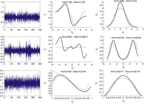
Fig. 1. ProcessesV(i),i =4,5,6 given inTable 1. First column: Difference between the integrated and discretized. True (bold), estimates using the integrated (thin grey) and the exact discretized (dotted thin) forb(second column) and
σ2(third column). Error values: “Int” for the integrated and “Disc” for the exact discretized.
Fig. 1shows in a few cases (forV(4),V(5)andV(6)) the differencesV¯k−Vk1(first column).
Clearly, these differences look like white noises forV(4)andV(6)and this was also true forV(1),
V(2),V(3)andV(7). OnlyV(5)seems to suffer from a lack of stationarity implying some peaks. In any case, the approximation ofVk1byV¯k does not suffer from any systematic bias. The last columns of Fig. 1plot the estimated curves obtained when using the Vk1’s or the V¯k’s, with associated error values. The estimated curves are very close.
Table 3compares more directly the performances of the different bases [T], [GP] and a mixed
strategy [M]. In [M], the algorithm chooses between the basis [T] and [GP], looking at the global penalized least square criterion value. The table gives the relative differences 100[(risk
−smallest risk)/smallest risk], which is a percentage of degradation with respect to the best score. Consequently, the best basis corresponds to a null value. The basis [GP] appears to be better than [T]: both have approximately the same number of null scores but errors with [T] may be large. The mixed strategy is slightly better, but it does not really outperform [GP]. Sometimes the mixed strategy performs worse than one of the individual strategy: this is probably due to the fact that [GP] is a local strategy, [T] is global and the algorithm chooses between [T] and [GP] via a global criterion.
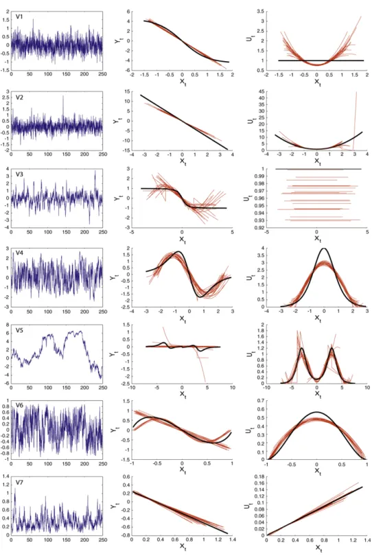
Lastly, inFig. 2, we have plotted the sample paths ofV(1), . . . ,V(7), the true functionsband
σ2(bold lines) together with 20 estimated functions based on the data pointsV¯
kusing the mixed strategy [M].
Fig. 2. First column: one path of the processesV(i),i=1, . . . ,7 given inTable 1. Second column: trueb(bold) and 20 estimations ofb. Third column: trueσ2and 20 estimations ofσ2.
Table 3
(Risk−Best Risk)/Best Risk with Trigonometric [T], General Piecewise Polynomial [GP] or Mixed [M] bases
b σ2 [T] [GP] [M] [T] [GP] [M] V(1) 49 0 1 0 2 4 V(2) 140 0 0 4 0 5 V(3) 0 65 46 0 224 231 V(4) 0 1 0 0 47 1 V(5) 0 7 14 13 0 16 V(6) 0 9 14 3 0 0 V(7) 797 0 0 400 0 0 6. Proof ofProposition 2.1
Consider the diffusion process(Vv0
t )given by dVt =b(Vt)dt+σ (Vt)dWt,V0 =v0and set
xu=1−(1/2)(Vuv10 −v0),u∈ [0,1]. Then,(xu)is the solution of dxu= ¯b(xu)du+ ¯σ (xu)dW¯u, x0=0,
withb¯(x) = 11/2b(x11/2+v0),σ (¯ x) = σ(x11/2+v0)and(W¯u)is a standard Brownian motion. Then, setting
U = Z 1 0 xudu, V =x1, we have (1/1) Z 1 0 Vv0 s ds=v0+11/2U, V1v0 =v0+11/2V.
Now, the following result is proved in ([21], Theorem 4). The random couple(U,V)has a joint densitypv0
1(u, v)such that
c−11exp(−c1(u2+v2))≤ p1v0(u, v)≤c−21exp(−c2(u2+v2)),
where the constantsc1,c2only depend on the bounds ofb, σand their derivatives. Consequently, the marginal density ofU, saypv0
U,1(u)satisfies
c01exp(−c1u2)≤ pvU0,1(u)≤c
0
2exp(−c2u2), (26)
withc0i = c−i 1(π/ci)1/2,i = 1,2. After an elementary change of variable, we get that the conditional density ofV¯0givenV0=v0, which is exactly the density ofv0+11/2U, is equal to
¯
v→ 1
11/2p
v0
U,1((v¯−v0)/11/2).
The densityπ¯1is obtained by integrating the above density with respect toπ(v0)dv0. Using the bounds(26), we obtain c01 Z R exp(−c1t2)π(v¯+t11/2)dt≤ ¯π1(v)¯ ≤c02 Z R exp(−c2t2)π(v¯+t11/2)dt. (27)
The stationary densityπ(.) is bounded and this gives an upper bound forπ¯1. Using (27), we have, for allt0>0,
¯
π1(v)¯ ≥c01
Z t0
0
exp(−c1t2)π(v¯+t11/2)dt.
Hence, for allv¯ ∈ [a,b],π¯1(v)¯ ≥ C0infu∈[a,b+t0]π(u)for some constantC
0. This gives the
result.
7. Proof ofTheorem 3.1 7.1. A list of auxiliary results
We shall need all along the proofs the following results and decompositions, which are proved in Section8. First V(k+1)1= ¯Vk+ 1 1 Z (k+1)1 k1 (u−k1)dVu. (28) Noting thatV(k+3)1−V(k+2)1=R(k +3)1
(k+2)1 dVu, and using(28), we get
Yk(+1)1= 1 12
Z (k+3)1
(k+1)1
ψ(k+1)1(u)dVu, (29)
whereψk1is given in(9). Second:
Lemma 7.1. Under assumptions[A1]–[A3], for all s,t ,|t −s| ≤1,E(Vt −Vs)2i ≤c|t −s|i
andE(V(k+1)1− ¯Vk)2i ≤c1i for i≤6and for any integer k.
Now, we state some useful lemmas required in the main proof. The remainder termsR(ki1),i =1,2 are defined by(10)and(12).
Lemma 7.2. Under Assumptions [A1]–[A3], E[(Z(k11))2] = (2/31)Eσ2(V0), E[(Z
(2,1) k1 )2] ≤
c1E(σ4(V0))andE[(Zk(21,2)) 2] ≤c
21, where the ci’s neither depend on k nor on1.
Lemma 7.3. Under Assumptions[A1]–[A3],
(a) E[(R((1k)+1)1)2] ≤c11andE[(R( 1)
(k+1)1)4] ≤c
0
112,
(b) E[(R˘(k+1)1)2] ≤c212andE[(R˘(k+1)1)4] ≤c2014for R defined by˘ (12), (c) E[(σ2(V(k+1)1)−σ2(V¯k))2] ≤c31andE[(σ2(V(k+1)1)−σ2(V¯k))4] ≤c0312, (d) E[(R((k2)+1)1)2] ≤c41andE[(R((k2+)1)1)4] ≤c
0
412
where ci and c0i neither depend on k nor on1, for i =1, . . . ,4.
The order obtained inLemma 7.3(c) is worse than the one obtained inLemma 7.3(b) and is not enough to reach optimal rates in the risk bounds. Nevertheless, if the functions ofSm are at least twice differentiable, then we obtain a better result by using another approach.
Lemma 7.4. Let Tn(t)= 1 n n X k=1 (σ2(V (k+1)1)−σ2(V¯k))t(V¯k). (30)
Then, under Assumptions[A1]–[A4]and[A6]–[A7], and if 1 ≤ n−2/3for[T]or 1≤ n−3/4 for[W], then, for the maximal spaceSnof the collection,
E sup t∈Sn,ktk=1 Tn2(t) ! ≤ c n. (31) 7.2. Proof ofTheorem 3.1 Recall thatktk2 ¯
π =R t2(x)π¯1(x)dx(see(7)). The regression contrast(13)may be written as:
γ(i) n (t)−γn(i)(f(i))= kt− f(i)k2n− 2 n n X k=1 (Yk(+i)1− f(i)(V¯k))(t− f(i))(V¯k). In view of(10), let us introduce the two processes indexed by functionst:
ν(i) n (t)= 1 n n X k=1 t(V¯k)Z((ki)+1)1 and R( i) n (t)= 1 n n X k=1 t(V¯k)R((ki)+1)1. (32) Using the above notations, we obtain that, fori=1,2,
γ(i)
n (t)−γn(i)(f(i))= kt− f(i)k2n−2ν(ni)(t− f(i))−2Rn(i)(t− f(i)). (33) Note that fm(i) and fˆm(i) are both A-supported, so that when kf(i)1Ackn appears in both sides of an inequality, we can cancel it. By simply writing that γn(i)(fˆm(ˆi))+pen(i)(mˆ(i)) ≤
γ(i)
n (fm(i))+pen(i)(m), for allminMn, we obtain
k ˆf(ˆi) m(i)− fA(i)k 2 n ≤ kfm(i)− f( i) A k 2 n+2k ˆf( i) ˆ m(i) − fm(i)kπ¯ sup t∈Sm(ˆi)+Sm,ktkπ¯=1 ν(i) n (t) +2k ˆf(i) ˆ m(i)− f (i) m kn v u u t 1 n n X k=1 [R((ik)+1)1]2+pen(i)(m)−pen(i)(mˆ(i)) ≤ kfm(i)− fA(i)k2n+1 8k ˆf (i) ˆ m(i)− fm(i)k2π¯ +8 sup t∈Sm(ˆi)+Sm,ktkπ¯=1 [νn(i)(t)]2 +1 8k ˆf (i) ˆ m(i)− fm(i)k2n+ 8 n n X k=1 (R((ki)+1)1)2+pen(i)(m)−pen(i)(mˆ(i)).
Let us consider the set Ωn= ( ω ktk2 n ktk2π¯ −1 ≤ 1 2,∀t∈ ∪m,m0∈Mn(Sm+Sm0)/{0} ) . (34)
We use that, onΩn,ktkπ¯ ≤ √ 2ktkn, and thatk ˆf(ˆi) m(i) − f (i) m k2n ≤ 2(k ˆf( i) ˆ m(i) − f (i) A k 2 n+ kf( i) A −
fm(i)k2n). After some elementary computations, we get 1 4k ˆf (i) ˆ m(i)− fA(i)k 2 n1Ωn ≤ 7 4kf (i) m − f( i) A k 2 n+8 sup t∈Sm(iˆ )+Sm,ktkπ¯=1 [νn(i)(t)]21Ωn +8 n n X k=1 [R((ki)+1)1]2+pen(i)(m)−pen(i)(mˆ(i)).
ByLemma 7.3(a) fori =1, or (d) fori=2,E[(R((ik)+1)1)2] ≤c1.Taking expectation and using
[A5] yield E(k ˆfm(ˆi()i) − fA(i)k 2 n1Ωn)≤7π¯1kf( i) m − f( i) A k 2+32 E sup t∈Sm(iˆ )+Sm,ktkπ¯=1 [νn(i)(t)]21Ωn ! +32c01+4(pen(i)(m)−E(pen(i)(mˆ(i)))). (35) To control the supremum of νn(i)(t) on a random ball (which depends on the random mˆ(i),
i =1,2), we use the following result.
Proposition 7.1. Under the assumptions of Theorem3.1, there exists a numerical constant κ˜i such that, for p(i)(m,m0)= ˜κiσ2i
1 [Dm+(1+Lm0Dm0)]/(n12−i), we have E[(( sup t∈Sm+Sm(ˆi),ktkπ¯=1 ν(i) n (t))2−p(i)(m,mˆ(i)))1Ωn]+≤cσ 2i 1 Σ n12−i +c 0121 {i=2}, withΣ=P m0∈M ne −Lm0Dm0.
The proof of Proposition 7.1 is highly technical but follows the lines of the proofs of Proposition 6.1 and Lemma 6.2 fori = 1 and of Proposition 6.2 and Lemma 6.3 for i = 2 in [10], and is therefore omitted. For details, see also [11].
Making use of the functionp(i)(m,m0), we write
[ sup t∈Sm+Sm(iˆ ),ktkπ¯=1 ν(i) n (t)]21Ωn ≤ [(( sup t∈Sm+Sm(iˆ ),ktkπ¯=1 ν(i) n (t))2−p(i)(m,mˆ(i)))1Ωn]+ +p(i)(m,mˆ(i)).
Then the penalty pen(i)(.) is chosen such that 32p(i)(m,m0) ≤ 4(pen(i)(m)+pen(i)(m0)).
The result ofTheorem 3.1 on Ωn follows fromProposition 7.1 with pen(i)(m) ≥ κiσ12i(1+
Lm)Dm/(n12−i), and κi = 32κ˜i. Indeed, this choice ensures that for all m,m0 in Mn, 32p(i)(m,m0)≤4pen(i)(m)+4pen(i)(m0). Thus,
E(k ˆfm(ˆi(i)) − fA(i)k 2 n1Ωn)≤7π¯1kf (i) m − f( i) A k 2+8pen(i)(m)+c0σ2i 1 Σ n12−i +32c 01. (36) Lastly we need to check thatE(k ˆfm(ˆi()i)− fA(i)k2n1Ωc
n)≤c/n.
First, we look atΩnc. In Lemma 6.1 of [10], it is proved that, under our set of assumptions, P(Ωnc)≤ ˜c/n4. The constraint [A7] onNnis imposed here. The existence of the maximal space
Sn, [A4] and [A5] are especially needed and the constantc˜depends onπ¯0,π¯1and the mixing rateθ.
Then, we write the regression model (10) as Yk(+i)1 = f(i)(V¯k) +ε((ik)+1)1 with ε
(i) k1 =
Zk(i1) +Rk(i1). Let us recall thatΠm denotes the orthogonal projection (with respect to the inner product ofRn) onto the subspace ofRn,{(t(V¯1), . . . ,t(V¯n))0,t ∈ Sm}. By definition of fˆm(i), we have(fˆm(i)(V¯1), . . . ,fˆm(i)(V¯n))0 =ΠmY(i)whereY(i) = (Y2(i), . . . ,Y(
i) n+1)
0. Denoting in the
same way a functiont and the vector (t(V¯1), . . . ,t(V¯n))0, we can see thatkfA(i)− ˆfm(ˆi(i))k2n =
kfA(i)−Πmˆ(i) fA(i)k2 n+ kΠmˆ(i)ε(i)k2n≤ kf( i) A k2n+n −1Pn+1 k=2[ε( i)
k1]2. Using thatP(Ωnc)≤ ˜c/n4and [A6], we have: E(kfA(i)k2n1Ωc n)≤E 1/2[(f(i)(V¯ 0))4]P1/2(Ωnc)≤ c n2. (37) Next, E[(εk(i1))21Ωnc] ≤ E 1/2[(ε(i)
k1)4]P1/2(Ωnc). From Lemma 7.3(a) for i = 1 and (b) and (d) for i = 2, we know that E[(Rk(i1))4] ≤ c012. Moreover E[(Zk(11))4] ≤ cσ14/12. Thus, E[(ε(k11))4] ≤C0/12. On the other hand,E[(ε(k21))4]can be bounded by a constant independent of
kand1. This implies, by using thatn1≥1, that E h kfA(i)− ˆf(ˆi) m(i)k 2 n1Ωc n i ≤ c n. (38)
Inequality (18) of Theorem 3.1 follows by gathering (36) and (38) for the cases Bn(i) =
O(1)+O(1/(n12−i)).
As we have seen in the discussion of Section4, the termBn(2,1) =O(1)+O(1/n)is not small enough to recover optimal rates.
Therefore, we must improve the bound for Bn(2,1). This is possible for [W] and [T] only. We rewrite equality(33)using(12)as follows:
γ(2) n (t)−γn(2)(f(2))= kt− f(2)k2n−2νn(2)(t− f(2))−2Rn(t− f(2))−2Tn(t− f(2)), where Rn(t)= 1 n n X k=1 ˘ R(k+1)1t(V¯k),
andTn(t)is defined by(30). By the steps leading to(35), we obtain: E(k ˆfm(ˆ2()2)− fA(2)k 2 n1Ωn)≤ 7π¯1kf( 2) m − f( 2) A k 2+32c012+4(pen(2)(m)− E(pen(2)(mˆ(2)))) +32E sup t∈Sm(ˆ2)+Sm,ktkπ¯=1 [ν(2) n (t)] 21 Ωn ! +32E sup t∈Sm(ˆ2)+Sm,ktk=1 [Tn(t)]2 .
The term 32c012comes fromRn(t)andLemma 7.3(b). There is a new term involvingTn(t). UsingLemma 7.4and
E sup t∈Sm,m(ˆ2),ktk=1 [Tn(t)]2 ! ≤E sup t∈Sn,ktk=1 [Tn(t)]2 ! ,
8. Proofs of the auxiliary results
8.1. Proof ofLemma 7.1
From the strict stationarity, it is enough to prove that for 0≤t≤1,E(Vt−V0)2i ≤cti. This follows from the assumptions and standard applications of H¨older and Burkholder–Davis–Gundy inequalities.
8.2. Proof ofLemma 7.2.
First, E[(Zk(11))2] = (1/14)Rk(1k+2)1ψk21(u)E(σ2(V0))du, which gives the result as
R(k+2)1
k1 ψ 2
k1(u)du=213/3.
Note that 0≤ψk1(u)≤1. Now, by using the Burkholder–Davis–Gundy inequality, E[(Z(k21,1)) 2] ≤cσ4 1. E[(Z(k21,2)) 2] ≤ 19 12E Z (k+2)1 k1 ψ2 k1(u)σ2(Vu)b2(Vk1)du ! + 9 16E " Z (k+2)1 k1 Z (k+2)1 s ψ2 k1(u)du ! ((σ2)0σ )( Vs)dWs #2 ≤ 181σ12E[b2(V0)] + 18 16 Z (k+2)1 k1 [213]2E[((σ2)0σ )2(V0)]ds≤c1. For the moments of order 4, they are bounded forZ(2,1)and of order12forZ(2,2).
8.3. Proof ofLemma 7.3
Proof of (a). Using(29), and noting that 1
12
Z (k+2)1 k1
ψk1(s)ds=1,
we can see that, in decomposition(10), the residual term can be written asR(k11) =P2 j=1R( 1,j) k1 with R((1k+,11))1 =b(V(k+1)1)−b(V¯k), R((1k+,21))1 = 1 12 Z (k+3)1 (k+1)1 ψ(k+1)1(s)(b(Vs)−b(V(k+1)1))ds. For the first term, use the Taylor formula,Lemma 7.1and [A1] to obtain
E[(R((k1,+11))1) 2] = E " (V(k+1)1− ¯Vk) Z 1 0 b0(V¯k+u(V(k+1)1− ¯Vk))du #2 ≤ KE h (V(k+1)1− ¯Vk)2 i ≤ K01. (39)
It follows from [A1] andLemma 7.1that E[(R((1k,+21))1) 2] ≤cZ (k+3)1 (k+1)1 E[(Vs−V(k+1)1)2] ds 1 ≤c 01.
Proof of (b). We use again(29)to computeYk(2+)1given by(3) and exhibit the remainder term
˘
R(k+1)1. More precisely, we have:R˘k1= ˘Rk(11)+ ˘R( 2) k1+ ˘R( 3) k1with ˘ Rk(11)= 3 213 Z (k+2)1 k1 ψk1(s)b(Vs)ds !2 , ˘ Rk(21)= 3 13 Z (k+2)1 k1 ψk1(u)(b(Vu)−b(Vk1))du ! Z (k+2)1 k1 ψk1(u)σ(Vu)dWu ! , ˘ Rk(31)= 3 213 Z (k+2)1 k1 Z (k+2)1 s ψ2 k1(u)du ! τb,σ(Vs)ds,
whereτb,σ =(σ2/2)(σ2)00+b(σ2)0.Lemma 7.3(b) holds ifE[(R˘(ki1))2] ≤ci12fori =1,2,3. We only study the first one. The other terms are treated analogously by standard tools using [A1] and the moment assumption [A3].
E[(R˘(k11)) 2] ≤ 18 13 Z (k+2)1 k1 ψ4 k1(s)dsE(b 4(V 0))≤c12, using [A1], E(V04) < +∞, and R((kk++13)1)1ψ
4
k1(s)ds = 21
5/5. Analogously, we have E[(R˘k1)4] ≤c14. ThereforeLemma 7.3(b) is proved.
Proof of (c). From standard results on Euler schemes, using that(σ2)0σ is Lipschitz, it is known that: σ2(V (k+1)1)−σ2(Vk1)= √ 1(σ2)0( Vk1)σ (Vk1)ξk+ ˜R(k1) whereξk = 1−1/2(W(k+1)1−Wk1)andE[(R˜(k1))
2] ≤ c12. Moreover, from [19, Proposition 2], and the Taylor formula, we easily deduce that
σ2(V¯ k)−σ2(Vk1)= √ 1(σ2)0( Vk1)σ (Vk1)ξk0+ ˜R( 2) k , (40) whereξk0 =1−3/2R(k+1)1 k1 [(k+1)1−s]dWs andE[(R˜ (2)
k )2] ≤c12. Therefore, the following holds: σ2(V (k+1)1)−σ2(V¯k)= √ 1(σ2)0( Vk1)σ (Vk1)(ξk−ξk0)+ ˜Rk, (41) withE[(R˜k)2] ≤ c012. Noticing thatE[(ξk −ξk0)2] = 1/3, we get the first part of the result. Analogous tools allow us to complete the proof.
Proof of (d). This is a straightforward consequence of (b), (c) and Eq.(12).
8.4. Proof ofLemma 7.4
We only do the proof for [T]. Considering Sm in collection [T], we have to bound E supt∈Bm(0,1)[Tn(t)]2 where Bm(0,1) = {t ∈ Sm,ktk = 1}. We shall use the following
properties of the trigonometric basis and of collection [T] which can be checked by elementary computations. X λ∈Λm (ϕ(k) λ )2 ∞ ≤C D2km+1,kt(k)k∞≤C Dkm+1/2ktk, (42) kt0k ≤C Dmktk. (43)
We use decomposition(41)to splitTn(t)into
Tn(t)= ˜Tn(t)−E(T˜n(t))+E(T˜n(t))+ 1 n n X k=1 ˜ Rkt(V¯k), withT˜n(t)= 1nPnk=1 √
1[(σ2)0σ](Vk1)(ξk−ξk0)t(V¯k). Using(42)fork=0, we get
E sup t∈Bm(0,1) 1 n n X k=1 ˜ Rkt(V¯k) !2 ≤C Dm 1 n n X k=1 E(R˜2k) ! ≤C0Dm12.
Then notice that
E(T˜n(t))=E √ 1 n n X k=1 [(σ2)0σ](Vk1)(ξk−ξk0)(t(V¯k)−t(Vk1)) ! .
Here, we have to use two derivatives oft. We use Gloter’s decomposition again in order to write, as for(40), that
t(V¯k)−t(Vk1)=
√
1t0(Vk1)σ (Vk1)ξk0+ek(t). (44)
For anyt ∈ Sm,(42)fork =2 impliesEsupt∈Bm(0,1)e 2 k(t) ≤ C12D5m. Thus, with(43), we obtain sup t∈Bm(0,1)E [ ˜Tn(t)] !2 ≤K(Dm212+Dm513). (45) Next we write ˜ Tn(t)−E(T˜n(t))= ˜Tn(1)(t)+ ˜T( 2) n (t)−E(T˜( 2) n (t)) with a centered term
˜ Tn(1)(t)=1 n n X k=1 √ 1[(σ2)0σ](Vk1)t(Vk1)(ξk−ξk0),
and the noncentered term (already used above)
˜ Tn(2)(t)=1 n n X k=1 √ 1[(σ2)0σ](Vk1)(ξk−ξk0)[t(V¯k)−t(Vk1)].
Using the H¨older inequality and the fact thatTn(1)(t)is a sum of uncorrelated variables, we see that E sup t∈Bm(0,1) ˜ Tn(1)(t) !2 ≤ X λ∈Λm E ˜ Tn(1)(ϕλ)2 ≤ 1 n X λ∈Λm E[(ξ1−ξ10)2]E{[(σ2) 0σ]2(V 1)ϕλ2(V1)} ≤ 1 3 C Dm1 n E{[(σ 2)0σ]2(V 1)} :=c1Dm n . (46)
Next, using(44), we introduce more terms:
˜ Tn(2)(t)= ˜Tn(3)(t)+ ˜Tn(4)(t)+ ˜Tn(5)(t) with, sinceE[(ξk−ξ0 k)ξ 0 k] =1/6, ˜ Tn(3)(t)= 1 n n X k=1 1[(σ2)0σ2t0](Vk1)[(ξk+ξk0)ξ 0 k−E[(ξk+ξk0)ξ 0 k]], ˜ Tn(4)(t)= 1 6n n X k=1 [(σ2)0σ2t0](Vk1), T˜n(5)(t)= √ 1 n n X k=1 [(σ2)0σ](Vk1)ek(t). The last term is bounded by
E sup t∈Bm(0,1) [ ˜Tn(5)(t)−E(T˜n(5)(t))] !2 ≤ 4cE1/2{[(σ2)0σ]4(V1)}13D5m =c013D5m. (47)
MoreoverE(T˜n(3)(t))=0 and by using(42)withk=1, it follows that
E sup t∈Bm(0,1) ˜ Tn(3)(t) !2 ≤ X λ∈Λm E{[ ˜Tn(3)(ϕλ)]2} ≤ cξ1 2 n X λ∈Λm E{[(σ2)0σ2]2(V1)(ϕλ0)2(V1)} (48) ≤ C D 3 m12 n E{[(σ 2)0σ2]2(V 1)} :=c00D 3 m12 n , (49) where cξ = E[(ξ1 −ξ0 1) 2(ξ0 1)
2]. For the last term, we apply Viennet’s mixing covariance inequality (see Theorem 2.1, p. 472 and Lemma 4.2, p. 481 in Viennet [27]). There exists a functionb(1V)such that
E sup t∈Bm(0,1) [ ˜Tn(4)(t)−E(T˜n(4)(t))] !2 ≤12 X λ∈Λm Var 1 n n X k=1 [(σ2)0σ2ϕλ0](Vk1) !
≤ 41 2 n X λ∈Λm Z (ϕ0 λ)2(v)[(σ2)0σ2]2(v)b(1V)(v)dPV1(v) ≤ 41 2C D3 m n s X k kβV(k1)E1/2{[(σ2)0σ2]4(V1)} :=c31 D3m n . (50)
It follows from(45)–(47),(49)and(50)that
E sup t∈Sm,ktk=1 Tn(t) !2 ≤C D2m12+1Dm n +1 3D5 m+ Dm312 n + 1Dm3 n .
Since1 ≤ 1, D3m12/n ≤ D3m1/n. We have 1Dm/n ≤ 1Dm3/n. Using that Dm ≤ Nn ≤
√
n1≤n1, we get1Dm3/n≤12D2m. This implies E sup
t∈Sm,ktk=1
Tn2(t)
!
≤CD2m12+13D5m. (51)
If1≤n−2/3, replacingDmbyNnin the right-hand side of(51), we obtain thatNn212+Nn513≤
c/nand(31)follows.
For [W], since the constraint on Nn is different (Nn ≤ n1/ln2(n)), we get (31) for
1≤n−3/4.
References
[1] M. Abramowitz, I.A. Stegun, in: Milton Abramowitz, Irene A. Stegun. (Eds.), Handbook of Mathematical Functions with Formulas, Graphs, and Mathematical Tables, John Wiley and Sons, Inc, New York, 1972.
[2] Y. A¨ıt-Sahalia, Estimating continuous-time models with discretely sampled data, in: Richard Blundell et al. (Eds.), Advances in Economics and Econometrics, Theory and Applications, Ninth World Congress, vol. III, in: Econometric Society Monographs, vol. 43, Cambridge University Press, Cambridge, 2007, pp. 261–327. [3] Y. A¨ıt-Sahalia, P.A. Mykland, Estimators of diffusions with randomly spaced discrete observations: A general
theory, Ann. Statist. 32 (2004) 2186–2222.
[4] Y. Baraud, F. Comte, G. Viennet, Model selection for (auto)-regression with dependent data, ESAIM Probab. Stat. 5 (2001) 33–49.
[5] A.R. Barron, L. Birg´e, P. Massart, Risk bounds for model selection via penalization, Probab. Theory Related Fields 113 (1999) 301–413.
[6] A. Beskos, O. Papaspiliopoulos, G.O. Roberts, Retrospective exact simulation of diffusion sample paths with applications, Bernoulli 12 (2006) 1077–1098.
[7] A. Beskos, O. Papaspiliopoulos, G.O. Roberts, P. Fearnhead, Exact and computationally efficient likelihood-based estimation for discretely observed diffusion processes (with discussion), J. R. Stat. Soc. Ser. B Stat. Methodol. 68 (2006) 333–382.
[8] A. Beskos, G.O. Roberts, Exact simulation of diffusions, Ann. Appl. Probab. 15 (2005) 2422–2444.
[9] B.M. Bibby, M. Jacobsen, M. Sørensen, Estimating functions for discretely sampled diffusion-type models, in: Handbook of Financial Econometrics, North-Holland, Amsterdam, 2002.
[10] F. Comte, V. Genon-Catalot, Y. Rozenholc, Penalized nonparametric mean square estimation of the coefficients of diffusion processes, Bernoulli 13 (2007) 514–543.
[11] F. Comte, V. Genon-Catalot, Y. Rozenholc, 2005, Nonparametric estimation for a discretely observed integrated diffusion model, Preprint MAP5 2006-11,http://www.math-info.univ-paris5.fr/map5/publis/titres06.html. [12] F. Comte,Genon-Catalot, Penalized projection estimator for volatility density, Scand. J. Statist. 33 (2006) 875–895. [13] F. Comte, Y. Rozenholc, A new algorithm for fixed design regression and denoising, Ann. Inst. Statist. Math. 56
(2004) 449–473.
[14] R.A. DeVore, G.G. Lorentz, Constructive approximation, in: Grundlehren der Mathematischen Wissenschaften [Fundamental Principles of Mathematical Sciences], vol. 303, Springer-Verlag, Berlin, 1993.
[15] S. Ditlevsen, M. Sørensen, Inference for observations of integrated diffusion processes, Scand. J. Statist. 31 (2004) 417–429.
[16] D.L. Donoho, I.M. Johnstone, G. Kerkyacharian, D. Picard, Density estimation by wavelet thresholding, Ann. Statist. 24 (1996) 508–539.
[17] O. Elerian, S. Chib, N. Shephard, Likelihood inference for discretely observed nonlinear diffusions, Econometrica 69 (2001) 959–993.
[18] V. Genon-Catalot, T. Jeantheau, C. Lar´edo, Stochastic volatility models as hidden Markov models and statistical applications, Bernoulli 6 (2000) 1051–1079.
[19] A. Gloter, Discrete sampling of an integrated diffusion process and parameter estimation of the diffusion coefficient, ESAIM Probab. Statist. 4 (2000) 205–227.
[20] A. Gloter, Parameter estimation for a discretely observed integrated process, Scand. J. Statist. 33 (2006) 83–104. [21] A. Gloter, E. Gobet, LAMN property for hidden processes: The case of integrated diffusions, Ann. Inst. H. Poincar´e
Probab. Statist. 44 (2008) 104–128.
[22] M. Hoffmann, Adaptive estimation in diffusion processes, Stochastic Process. Appl. 79 (1999) 135–163. [23] M. Kessler, Estimation of an ergodic diffusion from discrete observations, Scand. J. Statist. 24 (1997) 211–229. [24] M. Lefebvre, On the inverse of the first hitting time problem for bidimensional processes, J. Appl. Probab. 34 (1997)
610–622.
[25] L.C.G. Rogers, D. Williams, Diffusions, Markov Processes, and Martingales. Volume 2: Itˆo Calculus, in: Wiley Series in Probability and Mathematical Statistics, John Wiley & Sons, Chichester etc., 1987, XIV, 475. (English). [26] M. Sørensen, Prediction-based estimating functions, Econom. J. 3 (2000) 123–147.
[27] G. Viennet, Inequalities for absolutely regular sequences: Application to density estimation, Probab. Theory Related Fields 107 (1997) 467–492.