RESEARCH PAPER
Analysis of root growth from a phenotyping data set using a
density-based model
Dimitris I. Kalogiros1,2, Michael O. Adu3, Philip J. White1,4, Martin R. Broadley5, Xavier Draye6, Mariya Ptashnyk2, A. Glyn Bengough1,2 and Lionel X. Dupuy1,*
1 The James Hutton Institute, Invergowrie, Dundee DD2 5DA, UK
2 University of Dundee, School of Engineering, Mathematics and Physics, Dundee DD1 4HN, UK
3 Department of Crop Science, School of Agriculture, College of Agriculture and Natural Sciences, University of Cape Coast, Cape Coast, Central Region, Ghana
4 Distinguished Scientist Fellowship Program, King Saud University, Riyadh, Saudi Arabia
5 University of Nottingham, School of Biosciences, Sutton Bonington Campus, Loughborough LE12 5RD, UK 6 Earth and Life Institute, Université Catholique de Louvain, 1348 Louvain-la-Neuve, Belgium
*Correspondence: [email protected]
Received 25 August 2015; Accepted 22 December 2015
Editor: Adam Price, University of Aberdeen
Abstract
Major research efforts are targeting the improved performance of root systems for more efficient use of water and nutri-ents by crops. However, characterizing root system architecture (RSA) is challenging, because roots are difficult objects to observe and analyse. A model-based analysis of RSA traits from phenotyping image data is presented. The model can suc-cessfully back-calculate growth parameters without the need to measure individual roots. The mathematical model uses par-tial differenpar-tial equations to describe root system development. Methods based on kernel estimators were used to quantify root density distributions from experimental image data, and different optimization approaches to parameterize the model were tested. The model was tested on root images of a set of 89 Brassica rapa L. individuals of the same genotype grown for 14 d after sowing on blue filter paper. Optimized root growth parameters enabled the final (modelled) length of the main root axes to be matched within 1% of their mean values observed in experiments. Parameterized values for elongation rates were within ±4% of the values measured directly on images. Future work should investigate the time dependency of growth parameters using time-lapse image data. The approach is a potentially powerful quantitative technique for identifying crop genotypes with more efficient root systems, using (even incomplete) data from high-throughput phenotyping systems.
Key words: Density-based models, kernel-based non-parametric methods, model validation, optimization, root system architecture, time-delay partial differential equations.
Introduction
The identification of crop genotypes that can efficiently cap-ture soil water and nutrients has become a major focus of research (White et al., 2013b). Recent work has demonstrated,
for example, that crops with deeper root systems may have better water uptake efficiency, while shallower root sys-tems often improve phosphorus (P) uptake (Lynch and
This is an Open Access article distributed under the terms of the Creative Commons Attribution License (http://creativecommons.org/licenses/by/3.0/), which permits unrestricted reuse, distribution, and reproduction in any medium, provided the original work is properly cited.
© The Author 2016. Published by Oxford University Press on behalf of the Society for Experimental Biology.
This paper is available online free of all access charges (see http://jxb.oxfordjournals.org/open_access.html for further details)
at University of Nottingham on November 18, 2016
http://jxb.oxfordjournals.org/
Wojciechowski, 2015). However, plant roots serve many other functions. They must acquire other essential mineral elements (White et al., 2013a) and provide mechanical support to aer-ial stems (Dupuy et al., 2005a), while delivering nutrients for soil microorganisms through exudation and biomass turno-ver (van der Putten et al., 2013). They are able to achieve such functions in a vast heterogeneity of soil profiles and a wide range of soil physical, chemical, biotic and abiotic environ-ments. To grow and thrive in such diverse soil environments, plants adapt their root development to explore patches of nutrients (Wang et al., 2006), to explore cavities and pores to grow through hard soils (Stirzaker et al., 1996), to create spe-cialized structures (Hodge et al., 2009) and to establish mutu-alistic associations with a range of microorganisms to access nutrients that are not available to them (Richardson et al., 2000). Understanding what makes a root system more effi-cient is therefore a multifaceted problem, with many aspects remaining poorly understood.
To improve the root systems of crops, it is essential to find ways to observe and characterize their growth patterns. Sophisticated imaging techniques are now commonly used in root studies. These include magnetic resonance tomography, X-ray microtomography, neutron radiography for detailed analysis of root systems in situ, and visible light imaging in rhizotrons and minirhizotrons (Clark et al., 2011). Detailed visualization of root growth processes also reveals com-plex root geometries (Zhu et al., 2011). These complex root branching structures cannot be described easily as quanti-tative traits and, as a consequence, this represents a serious limitation to breeding for improved root system architectures.
Since root architectures are complex dynamic systems that have underlying patterns of growth, models may be used to interpret and analyse such root growth data (de Dorlodot et al., 2007). Complex root architecture arises from elemen-tary processes of root elongation and branching. Models allow us to derive complex patterns from simple growth rules, and inverse modelling can be used to estimate what combina-tion of elongacombina-tion rates and branching interval parameters may have given rise to any given root system structure that obeys the underlying model rules. Models may also help to overcome issues of incomplete image data sets caused by limitations of imaging systems (Wells et al., 2012). However, to estimate model parameters from data and derive quantita-tive traits that could be used for breeding and improvement of crop root systems, efficient optimization techniques must be developed. Previous studies have shown that the problem is challenging, because models that are too simple may be biased or limited to early developmental stages (Dupuy et al., 2005b) and optimization of models that are too complex can overfit the data and usually lead to multiple sets of param-eters that are equally optimal (Pedersen et al., 2010; Garré et al., 2012).
In this study, a framework to extract root growth param-eters from sets of images of root systems is presented. Our approach is to develop an optimization procedure to back-calculate the parameter values for elongation, gravitropic and branching rates that would give rise to an observed root density distribution. The framework is based on a set of
simple time-delay partial differential equations that describe the evolution of root length density distribution. Density estimation methods that are specific to the hierarchical root system structure have been developed so that models can be efficiently fitted to experimental data. The performance of a range of different optimization techniques was assessed based on the ability to retrieve growth parameters from simulated data. The methods were then applied to analyse the growth of
Brassica rapa L. subsp. trilocularis cv. R-o-18 roots.
Materials and methods
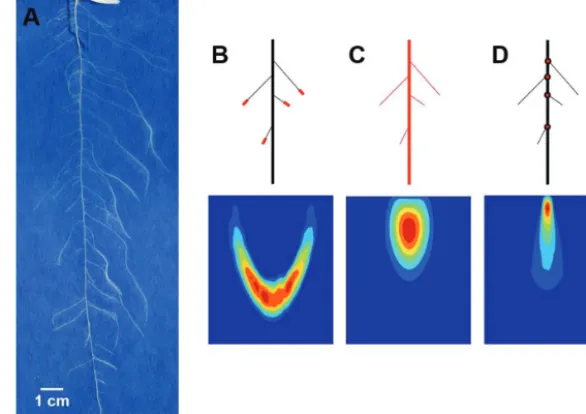
Root phenotyping dataData were derived from a previous set of experiments (Adu et al., 2014) in which seedlings of B. rapa L. subsp. trilocularis cv. R-o-18 were grown under standardized conditions on seed germination paper for up to 14 d after sowing and were scanned in five experi-mental trials using A4 CanoScan 5600F scanners (Canon UK Ltd, Reigate, UK). The young B. rapa root system skeleton consisted of a single primary root and a number of first-order lateral branches (Fig. 1A). The spatial position and angular orientation of roots were extracted from the segmented images of 89 plant root systems obtained via the semi-automated image analysis software SmartRoot (Lobet et al., 2011), which provided length measurements and topo-logical information about the root system. In the source image, after root tracing, root systems are divided by root trajectories that could comprise a finite number of line segments. Each line segment may be of variable length and is represented as two successive points described with their co-ordinates on the Cartesian plane. In order to build density distributions, the length, mid-point, and angle of each root segment were calculated. In total for the 89 plants, primary roots were made up of 22 290 individual line segments and lateral roots of 196 055 segments.
Elongation rates for the primary root and lateral roots were esti-mated directly from the total length and number of primary and lateral roots for each seedling using an established formula (Hackett and Rose, 1972). The elongation rate for primary root e(0) (cm d–1)
was determined as the total root length l(0) (cm) of the primary root
divided by 14 d, e( )0 l( )0 . 14
= The branching rate b(0) (d–1) was
deter-mined by counting the number n(1) of laterals per root system and
dividing by the time of growth after the emergence of the first lateral
root (11 d), b( )0 n( )1 .
11
= Finally, the elongation rate e(1) (cm d–1) for
laterals was evaluated by e l
n b
( ) ( )
( ) ( ) ,
1 1
0 0 2
2 11
= ⋅
⋅ ⋅ where l(1) is the lateral
root length determined from the tracing.
Description of the root system using density distribution functions
Estimation of model parameters through optimization is based on the ability to quantify differences between the experimental data and the model output. In order to quantify and then minimize such dif-ferences, a suitable mathematical representation of the root system density distribution functions must be derived. Here, the descrip-tion of the root system, both for the model and for the experimental data, used the notion of generalized densities following the con-cepts proposed by Dupuy et al. (2010a). Three fundamental quanti-ties were used to represent the root system: the root tip density ρa, the root length density ρl, and the root branching density ρb. The root tip density ρa (cm–3) indicates the number of root tips per unit
volume (Fig. 1B). The root length density ρl (cm–2) expresses the
overall length of roots per unit volume (Fig. 1C). The number of
at University of Nottingham on November 18, 2016
http://jxb.oxfordjournals.org/
connections between roots (i.e. branching points) per unit volume is represented by the root branching density ρb (cm–3) (Fig. 1D). The
root systems were grown on a flat surface forming a 2-dimensional structure. However, to describe both the spatial and angular distri-bution of roots, densities were defined in a generalized 3-dimen-sional space of R3, so that for each time t the function ρa (t,x,y,α)
defines the density of root tips at a horizontal position x and a ver-tical position y from the seed as well as in a direction of growth given by the root angle α, defined as the angle from the vertical axis. The branching order of roots is also defined, such that the primary root is of branching order 0 and laterals are of branching order 1. Root density distribution functions were also labelled according to their branching order with ρ( )ai , ρ( )li, and ρ( )bi denoting root tip, root length and root branching density of the roots of the ith order, respectively. In the following sections, upper indices will be omitted when an equation is valid for any given branching order.
Time-delay density-based root growth model for describing root density distributions
Root density distribution functions vary with time as a result of growth processes where root tips are created through branching and move as a result of elongation in a direction determined by gravit-ropism. A mathematical model adapted from the previously pub-lished model of Dupuy et al. (2010a) must therefore be defined to describe the changes in root densities as a function of these pro-cesses. Since the root system architecture is defined on a continuum, such models are derived using the concept of conservation of the root quantity in a volume Ω of R3. For any arbitrary
representa-tive volume Ω of R3 which is enclosed by a surface ∂Ω, the flux of
root tips across the surface ∂Ω can be expressed as a 3-dimensional vector F. In order to find a suitable expression for the flux F, one must consider that roots at a given location (x,y) and growth direc-tion α move only in one direction u = (sinα,cosα). The velocity of root tips is therefore (esinα,ecosα) where e (cm d–1) is the elongation
rate. However, at the same time, these same roots also change ori-entation as a result of gravitropism, which is assumed to be linearly related to the root angle based on semi-quantitative observations. The gravitropic rate is expressed as –gα, where g (d–1) is the
grav-itropic rate constant and the negative sign indicates the vertically downward direction. The flux of root tips is therefore expressed as F=ρa(esinα,ecosα,–gα). It is helpful to write the flux vector in the form:
F=eρa(sin cosα, α, )κ
withκ = −gα
e .
Since κ is the change in root angle divided by the change in root length (dα/dl), it is also the local curvature of the root (Dupuy, 2011). This relationship expresses the relationship between the elongation rate and the gravitropic rate on the morphology of the root system: both gravitropism and elongation are independent parameters, but it is the ratio between the two that determines the shape of the root system. The expression of the velocity field here differs slightly from previous papers (Dupuy et al., 2010a), because the angle α is defined from the vertical axis instead of the horizontal axis. Solutions to the problems, however, are unchanged. Thus, the conservation of the number of root tips for a given branching order i in an arbitrary representative volume Ω implies:
∂
∂t
∫
v+∂∫
⋅ S=∫
b vi i i
Ω Ω Ω
ρ( ) ( ) ( ) ,
a d F nd d (1)
where n is the unit normal vector to the surface element dS, and b
(cm–2 d–1) is the volumetric branching rate. Herein, the model
sug-gested by Dupuy et al. (2010b) is extended to incorporate a time delay in the emergence of lateral roots, which was experimentally observed in the branching patterns of B. rapa (Adu et al., 2014). Therefore,
∂tρa( )i =b( )i ,fori≥ 0and withb( )0 =0 (2)
and the source term b(i) for a given branching order i, using
nota-tions with explicit branching orders, is then expressed as a function of the root tip density of the previous branching order i–1:
bi b x y b t T x y b
ri i i i i i
( )=1 ( )− ( )−
(
+ ( ) − ( ))
+ ( )− −2
1 ρ 1 α 1 α
α α
a , , , ρa
(
, , (( ) − ( ))
,t Ti ,
witht T> ( )i. (3)
The constant br(i−1) represents the branching rate of roots of
branch-ing order i−1, and b( )i
[image:3.633.159.452.45.252.2]α designates the branching angle at which lateral
Fig. 1. The root system of a 14-day-old Brassica rapa seedling (L. subsp. trilocularis cv. R-o-18) comprising one tap root and multiple laterals grown on
seed germination paper (A). Schematic depiction of a root system made up of one tap root and four first-order laterals (upper picture) through the output variables of the density-based root growth model (lower picture). Illustration of the root density distributions through the corresponding maps: root tip density (B), root length density (C), root branching density (D).
at University of Nottingham on November 18, 2016
http://jxb.oxfordjournals.org/
roots of order i are initiated with a time delay denoted by T(i). In
our study, only one primary root per seedling (branching order i=0) and first-order lateral roots (branching order i=1) emerged during the experiment in the examined B. rapa root systems (i.e. i∈{ , }).0 1
Hence, the constant br(1 1−)or br( )0 refers to the branching rate of the
primary root (branching order i=0) and ba( )1 signifies the branching
angle at which the first-order laterals emerge, with a time delay given by T. The time delay T (instead of T(1) for simplification purposes)
was experimentally estimated from Adu et al. (2014). Root length density ρl and root branching density ρb are then derived from the root tip density ρa at a particular position X=(x,y,α) using the fol-lowing relationships: ρl=
∫
eρadt and ρb=∫
b td .Estimation of root tip density and root length density from root image data sets
It was necessary to quantify images of roots into experimental den-sity distributions for comparison with the model output.
Kernel density approach: A common approach to determine root densities consists of counting the number or length of roots falling in each cell of a spatial grid (Scott and Sain, 2005). The method is equivalent to making a histogram from a multidimen-sional data set. However, this method suffers from various limita-tions. Multidimensional histograms are less accurate because the method does not account for differences in position within a cell, the density estimates obtained are discontinuous and it is very difficult to derive an optimal grid, because such a process must consider not only the resolution of the grid but also the position and orientation of the grid in the multidimensional space. Herein, density distribution functions instead were derived using kernel density estimation. Kernel density estimation can be seen as a gen-eralization of the histogram approach with additional theoretical foundation. Kernel-based estimators differ from histograms in the following ways:
(i) A cell is viewed as a function, called kernel function, with non-zero values defined only in the neighbourhood of the centre of the kernel. For example, Gaussian or boxcar functions are clas-sically used to describe the values as a function of the distance from the kernel centre.
(ii) Kernel functions are not arranged in a grid but are adjusted so that they can be centred on each point of the data.
(iii) The sum of all the kernel functions provides the estimate for the density distribution function.
A histogram density estimate is therefore a boxcar kernel estimate for which the centres of the kernels are placed at the position of the nearest cell of a grid.
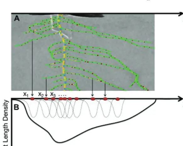
The method presented here was adapted not only to include the effect of changes in lengths of root segments but also to account for the specific structure of the spatial distribution of points derived from the digitiza-tion of the root system. SmartRoot (Fig. 2A) was used to produce the list of oriented root segments (Adu et al., 2014). Thus, only the spatial distribution of root segments was used in this study, not the connectivity between them. Even though SmartRoot was used to obtain root seg-ments, other software for image analysis could be used to provide similar data. The list of oriented root segments was then used to estimate a length density distribution function (Fig. 2B). In the experimental set-up, seed-lings did not have an identical position in the image. Therefore, co-ordi-nates of all root segments from one image were translated by a constant vector so that all root systems were aligned to where all the seeds were
located, at a unique position Lx2 ,0 (0,0) in the image. The position of the centre of the ith root segment of length li is denoted by Xi (Fig. 2B).
Then, the estimator of the root length density ρl
( )
Χ is constructedusing the following formula:
ρl i
m
i i
lW
( )
ΧΧ =(
−)
=
∑
,1
X X (4)
withΧΧ∈
[
,]
× , × − , .
0 0
2 2
Lx Ly L Lα α
Here, W (cm–2) is a kernel function and m indicates the total
num-ber of root segments. The kernel function W is usually a positive, even, unimodal real-valued function with a maximum at zero and integrates to 1 (i.e.
3
1
∫
WdX= ) (Xiao-Feng and De-Shuang, 2009).Fig. 2. Schematic representation of the method that yields the root length density estimate based on the skeleton of individual Brassica rapa roots
produced with SmartRoot. (A) Depiction of midpoints of consecutive line segments along the primary root (marked with X) as well as the laterals (denoted by dots). (B) Kernel estimation method for the root length density. The mid-points are the centres xi of the classical Gaussian kernels (dotted normal curves)
which sum up to the kernel estimator of the root length density (plain curve).
at University of Nottingham on November 18, 2016
http://jxb.oxfordjournals.org/
[image:4.633.167.459.461.694.2]For this study, the classical Gaussian kernel was chosen and defined as (Scott and Sain, 2005):
W
d
Χ Χ
ΣΣ ∑∑
( )
=( )
− − 1 2 1 2 1π exp X X ,
T
(5)
where |Σ| defines the determinant of the positive definite matrix
Σ, which is the covariance matrix in the d-dimensional generalized space. Since the variables x,y,α are independent and therefore uncor-related, Σ is a non-zero 3 × 3 diagonal of the form:
ΣΣ = k s s s x y 2 2 2 2 0 0 0 0
0 0 α
, (6)
where k is the scaling factor of the kernel density estimator and sx,
sy, sα are normalization factors which account for the different grid
spacing along the three dimensions x,y,α. Since k determines the smoothness of the density distribution function, we will also call it the spatial resolution. The density estimation depends on the param-eters k, sx, sy, and sα of the kernel function W (Hwang and Lay,
1994).
Optimal scaling factor for the kernel density approach: In order to match the kernel density function to the experimental data, an opti-mal value for the scaling factor (kopt) must be found. The optimal
scaling factor corresponds to the trade-off between overfitting of the data, which is obtained when values of k are too small, and a coarse representation of the data, when values of k are too large. This optimum was determined using a method called pseudo-log-likelihood cross-validation (Turlach, 1993). The pseudo-log-likelihood is a sta-tistical metric that indicates how well an estimate agrees with the data. It is calculated as the product of the probabilities of each of the model predictions on the data sets. The logarithm of the like-lihood is more commonly used in numerical applications because its expression is usually simpler. Since the scaling factor k depends on the data, there is no independent observation to determine the likelihood value. One way to overcome this limitation is to use the Leave-One-Out cross-validation method denoted by CVLOO.
In the Leave-One-Out cross-validation method, the density is esti-mated on all but one of the data points (j in Equation 7) and the log likelihood is determined on that missing point. The calculation is repeated for each point in the data set so that a global estimation of the log likelihood is obtained:
CV k
m j lW m
i j
i j i
LOO
( )
=−
(
−)
= ≠∑
∑
1 1 1log X X , (7)
where m denotes the total number of mid-points in a root system. Unfortunately, this method does not differentiate between root seg-ments belonging to the same root and root segseg-ments of two differ-ent roots. In order to address this problem, it is important to adopt a different approach to cross-validation. First, it is useful to use a different numbering for the root segments so that indices of roots and their segments appear explicitly in the summation. We therefore denote Xij and lij the co-ordinates and length of the jth root segment
on the ith root:
CV k
m i n
j m
r n s m s j r i
i i
LOO
( )
=− < ≤ < ≤
< ≤
< ≤ ≠ =
∑
1 10 0 0 0 , log for ,∑
(
−)
l Wrs Xij Xrs (8)
where n is the number of roots and mi is the number of segments on
the ith root, so that
i n i m m =
∑
= 1 .Traced roots show a high density of nodes on a single root but low point density between roots. To include this point cloud struc-ture, data points were subgrouped with respect to the roots to which they belong. A V-fold cross-validation (CVV-fold) method was used
to determine kopt. In a V-fold cross-validation (Geisser, 1975), entire
roots are omitted (r i≠ in Equation 9) for the determination of the pseudo-log-likelihood, and the cross-validation function is expressed as:
CV k
m i n l W X
j m
r n r i s m
rs ij rs
i i
V fold−
< ≤ < ≤
< ≤ ≠ < ≤
=
−
∑
∑
−( ) log , 1 10 0 0 0 X
((
)
. (9)
The optimal value of the scaling factor kopt maximizes the
pseudo-log-likelihood, CV
i m l i =
( )
=∏
log 1ρ X , so that:
kopt:=argmaxkCV k( ) (10)
The size of the elements of the finite volume grid was adjusted to correspond to the scale factor k identified by the V-fold cross-validation. In this setting, an increase in the grid resolution cannot lead to an improved fit since the resolution of the experimental data cannot be improved further.
Estimation of density-based model root growth parameters using optimization and comparison with the experimental data set The previous steps have established a mechanism to determine a root density distribution from root experimental data. In the next step, the objective was to determine the values of the root growth parameters that best reproduce the root length density distribution evaluated from the experimental data for roots of each branching order i (Equation 4). Experiments took place in a controlled environ-ment, for a short period of time (14 d), on seedlings that had already germinated for 3 d. Therefore, growth parameters were assumed to be constant. Differences between simulated density (ρl( )i ) and the density distribution function estimated from data (ρ( ))
l i
were quan-tified through a cost function E(i) dependent on the vector of model
parameters θθ( )i =
(
e( )i ,g( )i,b( )i)
. E(i) was defined as the squareddif-ference of the estimated and model-predicted density functions inte-grated over the entire domain V=( ,0Lx) ( ,× 0Ly) (× −L L, )
2 2
α α and
divided by the volume of the domain LxLyLα. For roots at branching
order i, the error E(i) was determined as:
E
L L L dxdyd
i
x y l
i l i V ( )= ( )− ( ) .
∫∫∫
1 2α ρ ρ α
(11)
The vector of optimal model parameters θθopt( )i was defined by
recurrence:
θθopt( )0 :=argminθ( )0 E( )0
( )
θθ( )0 ,(12)
θθopt( )i :=argminθ( )i E( )i
(
θθ( )opt0 , ,…θθ(opti−1),θθ( )i)
,0< ≤i n.This approach is exact because root length density at branching order i is independent of growth parameters for branching order
j, if i<j. Since models are solved numerically, optimization is com-putationally intensive. However, solving at each branching order separately allows the problem to remain computationally tractable. Root branching order can be derived experimentally using either
at University of Nottingham on November 18, 2016
http://jxb.oxfordjournals.org/
time-lapse data about root emergence or using classes of root diam-eter as a proxy for root branching order or elongation rate.
To determine the most efficient non-linear optimization algorithm, four different optimization methods were tested: Powell’s method, the Conjugate-Gradient method, the Broyden–Fletcher–Goldfarb– Shanno method (BFGS), and the Nelder–Mead method (Nelder and Mead, 1965).The root density at the start of the experiment was chosen as the initial root distribution for the model. When the true parameters are known, the quality Q of the fit can be defined as the ratio of the estimated parameter θˆ to the original model parameter
θ for the simulation so that optimal parameters were identified when
Q=1, with Qθ θ θ
( )
= .The calculated elongation rates were also compared with those derived by direct estimation based on the increase in root length den-sity for each order of root:
e t dt t dxdyd
dt dxdyd l l V a V . =
(
(
+)
−( )
)
×∫∫∫
∫∫∫
ρ ρ α
ρ α (13)
Since it is not usually possible to identify root tips from images of plants grown in soil, the number of root tips
∫∫∫
Vρadxdydα wasassumed to be constant for primary roots. This value is often known and consistent in seedlings of a given plant genotype.
Sensitivity analysis and confidence intervals for fitted density-based model root growth parameters of B. rapa
The method described in the previous section provides a single set of optimal root growth parameters that best reproduce the root length density distributions measured experimentally. Further analyses are required to determine how reliable the estimates of these growth parameters are. Therefore, sensitivity analysis was performed on model parameters. Sensitivity was assessed based on a 1% increase in each model base parameter value. The Model Elasticity Value (MEV) of the output error, which is specified as the percentage change in the cost function E (Equation 11) per percentage change in the model parameter p, was determined:
MEV := .
δ δ E E p p (14)
A bootstrap method was used to evaluate the confidence intervals of model parameters. Since the spatial distribution of mid-points was highly structured, data sets were re-sampled randomly following the V-fold sampling approach described previously. For each bootstrap sam-ple, the model was parameterized and parameter values were recorded. For each parameter, the bootstrap Standard Error (SE) was defined as:
SE= − − = −
∑
( ) ( ) , 1 1 1 2 1 2R R r p p
R
r (15)
where R is the total number of replications, pr denotes the estimated
parameter at replication r and p− is the mean parameter value. Then, 95% confidence intervals (CIs) were evaluated together with the coefficient of variation (CoV) for each of the model parameters.
Analysis of the performance of the optimization process
Two types of analyses of the optimization process were performed. First, the performance and testing of optimization algorithms was carried out using root growth simulation data (Fig. 3A) to create
a target root length density distribution function resulting from known model parameters. With the simulated data, it was possible to quantify directly the goodness of the fit of model parameters. Optimal model parameters were determined using various non-linear optimization algorithms. Once the performance of the algo-rithms was assessed, the algorithm with the faster convergence rate and improved accuracy was used for analysis of real experimental data. In a second step, the optimization algorithm was applied to real data with the experimental root density at t=0 chosen as the initial root distribution for the simulations. Estimation of model parameters from data, however, includes the additional kernel den-sity estimation step (Fig. 3B). The optimization process then follows the same set of steps. An optimization algorithm (Fig. 3C) deter-mines a set of candidate model parameters that are used to simu-late the root system (Fig. 3A), and the results of these simulations are compared with the target root system using the cost function (Fig. 3D). The optimization procedure (Fig. 3C and Fig. 3D) is iter-ated until convergence criteria are met.
Solutions of the model were obtained numerically using the upwind finite volume method presented in Dupuy et al. (2010b). Numerical simulations were carried out on a 3-dimensional domain
0 0
2 2
,Lx ,Ly L L, .
(
)
×( )
× − α αThe size of the domain was
deter-mined to match the experimental set-up presented in Adu et al. (2014), with Lx=15 (cm), Ly=22 (cm), andLα=32π
( )
rad . Spatialresolution of the grid was determined based on a scaling factor k
such that dx=k, dy=k, dα=gπk/e, and dt=Ck/e where the Courant– Friedrichs–Lewy number C is set to 0.5 (Courant et al., 1967).
The algorithms were implemented in the python SciPy library (http://www.scipy.org/) using a personal computer of 3.1 GHz CPU (IntelCore i5-2400 CPU @ 3.1 GHz) and 4 Gb RAM, comparing the target root length distribution obtained for specific user-defined values of model parameters with the length distribution derived from the numerical model at each grid point (Fig. 3). The relevant codes and experimental data can be found at http://www.archiroot. org.uk.
Results
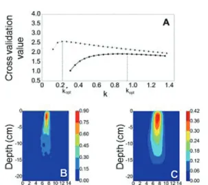
Kernel density estimates: V-fold cross-validation performed better than Leave-One-Out cross-validation Density estimations based on V-fold cross-validation and Leave-One-Out (LOO) cross-validation were obtained on the root length density both of primary root and of lateral roots. In each case, comparisons between the two methods were performed visually. The optimal scaling factor k'opt at
which the function CVLOO(k) attained its maximum (Fig. 4A)
was equal to 0.23 for primary and 0.20 for lateral roots. It produced patchy density distributions for both primary root and lateral roots (Fig. 4B). Estimation of total root length with both methods was very close to those measured experi-mentally, with values of 15.77 cm and 15.68 cm, respectively, obtained by LOO and V-fold cross-validation for the primary root, and values of 106.45 cm and 105.56 cm, respectively, for lateral roots. The measured total primary root length was 15.54 cm and the total lateral root length was 105.26 cm. The close match between model-estimated and measured total lengths showed only minor edge effects at the boundary of the domain. When the CVV-fold method was employed, the optimal
scaling factor kopt was equal to 0.9 for primary (Fig. 4A) and
0.57 for lateral roots. The method showed better compromise
at University of Nottingham on November 18, 2016
http://jxb.oxfordjournals.org/
Fig. 3. Diagrammatic representation of the suggested method for data-driven testing and estimation of the model parameters. The target root system architecture (RSA) is derived through the available data sets (experimental data) or from models for which model parameters are known (simulated data). Testing consists of using simulation with known parameters (A) to create a target root length density distribution function. When the target density distribution results from simulation, it is possible to compare directly the estimated model parameters to target parameters. Estimation of model parameters from data uses a density estimation step (B). The optimization process then follows the same set of steps. An optimization algorithm (C) determines a set of candidate model parameters that are used to simulate the root system (A), and the results of these simulations are compared with the target root system using a cost function (D). The optimization procedures (C and D) are iterated until a convergence criterion is met. Optimal model parameters were determined using non-linear optimization algorithms. The most efficient method which was proven to minimize the discrepancies between the target and the estimated RSA was then applied to experimental data in order to extract root growth parameters.
Fig. 4. Comparative performance analysis of Leave-One-Out and V-fold cross-validation methods on the optimal scaling factor k of the kernel estimator.
(A) For primary root, employing the Leave-One-Out grouping method, the cross-validation function CV(k) attains its maximum value at k'opt (dashed), while sampling based on the V-fold method yields the maximum CV(k) at kopt (plain). (B) Visualization of the root length distribution with scaling factor k'opt for the kernel estimator (Leave-One-Out method). (C) Visualization of the root length distribution with scaling factor kopt for the kernel estimator (V-fold method). The color map indicates the root length density and units of the colour bar are cm−1.
at University of Nottingham on November 18, 2016
http://jxb.oxfordjournals.org/
[image:7.633.149.453.383.653.2]between the bias and variance of the estimator, with density maps being smooth, yet not oversmoothed (Fig. 4C).
Factors that influence density-based model parameterization
Initially, optimization algorithms were applied to simulated density data with known growth parameters. The results showed that the direct estimation of the elongation rate e cal-culated from the change in the root length over time (Equation 13) was not accurate, and direct estimates of elongation rates decreased over time. The convergence to the true model param-eter was increased with improved grid resolution (data not shown), but root fluxes at the boundaries of the finite volume grid prevented accurate estimation of the elongation rate as roots grew out of the grid. Simplex-based optimization tech-niques, such as Nelder–Mead, performed better than gradient-based methods, such as Conjugate-Gradient or BFGS, which were slower to converge toward optimal parameters. Other widely used methods, such as the Powell’s conjugate direction method, proved to be less effective for this type of problem.
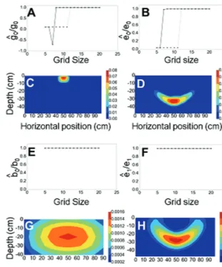
The fitting of the model by optimization was influenced by the resolution of the grid and the time of growth simulated in the model. First, there was a minimum grid size, below which optimization algorithms did not converge to the true model parameter (Fig. 5A, B). The results also showed that longer experiments provide better parameter estimation. For the Nelder–Mead algorithm, when the experiment lasted 15 d, the true value of the gravitropic rate constant g of the pri-mary root could only be obtained for grid elements (NY=12) along the depth (Fig. 5A), whereas for a 25 d experiment the same optimal value g was obtained at a lower grid resolution with NY=8 (Fig. 5A). Although good estimates for model parameters could be obtained using a small number of grid points, higher grid resolution is still required for accurate model predictions. For example, irrespective of the duration of the experiment, the optimal values of the branching rate
b of the primary root and the elongation rate e of first-order laterals were obtained at NY=5 (Fig. 5E, F). However, the representation of root density distribution at this resolution is too coarse for practical application (e.g. studies of geno-typic variation, nutrient uptake, or fertilizer applications).
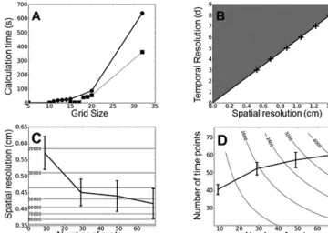
Calculation time, spatial and temporal resolution
Calculation time increased with the number of elements in the finite element grid on which the model was run. The increase was not linear because the model was run on 3-dimensional grids (Fig. 6A) and the complexity of calculation increased as a power of 3. There was a linear relationship between the mini-mum time interval at which a change in growth parameter can be detected and the spatial resolution of the grid (Fig. 6B). The scale factor k was determined on different numbers of root systems. This was achieved by removing roots randomly from the database and running the cross-validation algorithm on the reduced data set. Simulation showed that increasing the num-ber of roots reduced the scale factor k and therefore improved the spatial resolution (Fig. 6C, plain line). However, increasing
the spatial resolution involves additional resources to acquire more measurements (Fig. 6C, horizontal isolines). Based on the results in Fig. 6B and C, it is possible to determine the optimal combination of time points and replicate them in an experiment (Fig. 6D). The number of time points as a function of the num-ber of roots measured (replication) was calculated on the basis of a 100 d experiment. Increasing the number of roots measured at a given time point (replication) increases the spatial resolu-tion of the model, and this also allows for improved temporal resolution. However, the increase was not linear so that increas-ing both spatial and temporal resolution usually requires a large increase in the number of replicates. In general terms, this result suggests the number of replicates contributes more to resolution than the number of time points in an experiment (Fig. 6D).
Estimation of root growth parameters using a density-based model
The model was fitted on data from B. rapa roots of 89 plants, 22 290 and 196 055 mid-points for primary and lateral roots, respec-tively. The primary root elongation rate was 1.19 cm d–1 and the
gravitropic rate was 0.2 d–1. For lateral roots, the branching rate
was 3.52 cm d–1, the root branching angle directly measured on
image data was 7π/8, and the delay for lateral root initiation was 3 d. The optimal elongation rate and gravitropic rate of first-order laterals were 0.44 cm d–1 and 0.07 d–1, respectively.
The model-predicted total primary root length was 15.68 cm, while the estimated total root length was 15.54 cm. In addition, according to the model output, the total lateral root length per plant was 105.56 cm, whereas the real data-based estimate was 105.26 cm. Hence, the model slightly overestimated both the primary and lateral root length by 0.9% and 0.3%, respectively.
Accuracy of optimized root growth parameters for the density-based model
Root growth parameters obtained by optimization were com-pared with growth parameters estimated directly from the image data and the results showed that optimized param-eters matched the experimental paramparam-eters. The experi-mentally estimated elongation rate of the primary root was 1.15 ± 0.05 cm d–1 (n=89), which agreed with the
cor-responding optimized value of 1.19 cm d–1 obtained by
fit-ting the model parameters to the density data (see above). The experimentally estimated rate of increase in lateral root length was 0.45 ± 0.03 cm d–1 (n=89), which agreed with the
value of 0.44 cm d–1 obtained by fitting the model to the data
(see above). Sensitivity analysis also showed that predictions of the root length density varied differently for the same change in the elongation, branching, and gravitropic param-eters. In response to a 1% change in parameter values, such as elongation rate and branching rate for the primary root and the elongation rate of laterals, the cost function rose by 0.947%, 0.996%, and 0.972%, respectively (MEV in Table 1). Conversely, the error was less sensitive to the gravitropic rate for either primary or lateral roots. A change in the model parameters by 1% induced a 0.073% and 0.003% change in the error function (Table 1). Bootstrap analysis of the
at University of Nottingham on November 18, 2016
http://jxb.oxfordjournals.org/
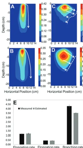
standard errors showed that all growth parameters were esti-mated within the 95% CI of the model parameter. Elongation rates and branching rate were very sensitive parameters with CIs and CoV smaller than those obtained for the gravitropic rates (Table 1). Overall, our method leads to a good fit of the mathematical model to the experimental root length density data (Fig. 7A–D) with reasonable parity between predicted and measured root growth parameter values (Fig. 7E).
Discussion
Using models to extract root growth parameters from experimental image data
Although the growth and development of individual roots is reasonably well understood, root system architectures
(RSAs) observed experimentally often show complex pat-terns that cannot be easily characterized or predicted. RSAs are not merely self-similar fractal structures that simple reit-eration of elongation and branching rules might predict. It is often observed, for example, that mortality and turnover are more frequent in thinner and higher order lateral roots (Norby and Jackson, 2000). Elongation and branching are also modulated by environmental and edaphic factors as well as systemic signals, so that more roots can be produced in regions of soils that are favourable to the plant such as local-ized nutrient patches (Hodge et al., 2009). Root growth can also be extremely variable, with, for example, 5- to 10-fold variations in elongation rates observed for lateral roots (Forde, 2009).
[image:9.633.147.459.38.413.2]Obtaining suitable information to describe the growth of RSAs is therefore essential, but to date it has been a relatively
Fig. 5. Estimation of root growth parameters on simulated data. (A) Quality of fit of the gravitropic rate estimate g
0 of primary roots against the number of grid elements NY for 25 d (plain line) and 15 d (dotted line). (B) Quality of fit of the elongation rate estimate e
0 of primary roots against the number of
grid elements NY for 25 d (plain line) and 15 d (dotted line). (C) Visualization of the primary root tip density after 15 d of growth with gravitropic rate g
0
=0.007 d–1 and e
0=0.07 cm d
–1, and number of grid elements NY=32. (D) Visualization of the primary root tip density after 15 d of growth with the expected
gravitropic rate g0 = 0.07 d–1, expected elongation rate e0 = 2 cm d–1, and number of grid elements NY=32. (E) Quality of fit of the branching rate estimate b 0 of primary roots against the number of grid elements NY for 25 d (plain line) and 15 d (dotted line). (F) Quality of fit of the elongation rate estimate e
1 of the
first-order laterals against the number of grid elements NY for 25 d (plain line) and 15 d (dotted line). (G) Visualization of the first-order lateral root tip density after 15 d of growth with number of grid elements NY=5 and branching rate of primary roots b0 = 2 d–1 and elongation rate of first-order laterals e1 = 2 cm d–1. (H) Visualization of the lateral root tip density after 15 d of growth with number of grid elements NY=20 and branching rate of primary roots b0=2 d–1 and elongation rate of first-order laterals e1=2 cm d–1. The color map indicates the root tip density, and units of the color bar are cm−2.
at University of Nottingham on November 18, 2016
http://jxb.oxfordjournals.org/
major (low-throughput) undertaking (Tsegaye and Mullins, 1994; Tsegaye et al., 1995; Pellerin and Pagès, 1996). For these reasons, it has been proposed that optimization methods could be used to invert mathematical models so that growth parameters can be obtained from the models (de Dorlodot et al., 2007). In the past, simple empirical root depth mod-els were used to fit root data extracted from soil cores. These models were rarely related to meaningful growth parameters that could explain the changes taking place in the root length density profiles through time. Reddy and Pachepsky (2001), Heinen et al. (2003), and Bonneu et al. (2012) have proposed the use of advection–diffusion equations to describe temporal changes in root spatial distribution in soil. In each case, the
methods proposed could reliably mimic the spread of the root system in soil, but the models used in these studies were very simple and could not provide information on parameters such as the branching rate or the elongation rate of lateral roots.
[image:10.633.128.489.42.298.2]More sophisticated architectural models have been pro-posed to explore whether a greater range of parameters can be extracted from mini-rhizotron data (Garré et al., 2012). However, when root architectural approaches are used, it is difficult to obtain the many architectural parameters to com-pare experimental with modelled root architectures. This is because root architectures, whether measured or modelled architecturally, are unique realizations of a stochastic process and there is no single obvious way to quantify their similarity. There have been various attempts to find ways of comparing RSAs: topological indicators such as magnitude and altitude (Fitter, 1987), fractal dimensions (Fitter and Stickland, 1992) or topological distances have all been proposed for direct comparisons between topologies (Ferraro and Godin, 2000), but they all fail to include a spatial representation of the root system. For these reasons, various forms of root density dis-tribution have been used to compare root systems. For exam-ple, Grabarnik et al. (1998) used root length profiles (root length distribution with depth) to describe root distribution. Garré et al. (2012) used root number density (normalized number of roots) to compare mini-rhizotron observations at various depths with model predictions.
Fig. 6. Calculation time, and spatial and temporal resolution. (A) Calculation time and quality of fit for the Nelder–Mead minimization method on simulated
data: at different grid sizes (number of grid elements NY) for 25 d (plain line) and 15 d (dotted line). (B) Relationship between the spatial and temporal resolution is obtained by determining the minimum time interval over which growth parameters can be estimated at a given spatial resolution. Crosses indicate simulated results and the plain line indicates the linear fit to the data. (C) Spatial resolution increases with the number of replicates, but increasing the resolution required an exponential increase in the number of roots measured. Horizontal isolines indicate the number of grid elements required to simulate the growth of root systems at a given spatial resolution. (D) Optimal number of time points as a function of the number of roots measured (replication) calculated on the basis of a 100 d experiment. Isolines indicate the total number of measurements in an experiment. The intersection of an isoline with the curve indicates the optimal sampling strategy for a given number of measurements. In general terms, this result suggests that it is usually more important to increase replication than the number of time points in the experiment.
Table 1. Sensitivity analysis of the estimated root growth parameters for primary root (e(0),g(0)) and lateral roots (b(0),e(1),g(1)) with the model elasticity value (MEV), the 95% confidence interval (CI) with sample size N = 100 and the coefficient of variation (CoV).
Parameter Units Estimate MEV SE CI CoV (%)
e(0) cm ⋅ d–1 1.189 0.947 0.0043 1.179–1.196 3.62 g(0) d–1 0.196 0.073 0.00043 0.195–0.197 2.17 b(0) d–1 3.521 0.996 0.0027 3.513–3.524 0.77 e(1) cm ⋅ d–1 0.441 0.972 0.00053 0.439–0.441 1.19 g(1) d–1 0.0708 0.003 0.00022 0.07–0.071 3.15
at University of Nottingham on November 18, 2016
http://jxb.oxfordjournals.org/
[image:10.633.45.300.475.550.2]Since some form of density estimation is required during an optimization process to compare a model with experiments, why not simulate the root system as a density distribution directly? This was the original idea of Reddy and Pachepsky (2001), Heinen et al. (2003), Bastian et al. 2008, and Bonneu et al. (2012). However, because their density model was a generic advection–diffusion equation, it was not possible for them to obtain biologically meaningful growth parameters from their model. In the current study, the mathematical
equations have been tailored to represent root systems so that growth parameters appear explicitly in the model. Because of this modification, it was possible to obtain accurate estimates of elongation rate, branching rate and gravitropic rate.
Accuracy of the estimated root growth parameters
[image:11.633.161.449.36.546.2]This study has shown that by using density-based mod-els, it is possible to extract root growth parameters such as
Fig. 7. Measured and predicted root length density for the primary root (A, B). Measured and predicted root length density for lateral roots (C, D). The
arrows illustrate mechanisms that may explain differences between experimental and predicted growth patterns. For the primary root, gravitropism induced non-smooth changes in root angles (A) that were not accounted for in the model (B). Lateral roots, on the other hand, seemed to have varying elongation rates through time (C) and these were not represented in the model (D). The color map indicates the root length density, and units of the color bar are cm−1. (E) Comparison between measured root growth parameters (black) and estimated root growth parameters (grey).
at University of Nottingham on November 18, 2016
http://jxb.oxfordjournals.org/
elongation rate, branching rate, and gravitropic rate directly from experimental density distribution functions. Although the data used to test the method were simple, they provided very useful information on growth parameters that can eas-ily be obtained from experimental root density distributions. The study showed that elongation rates of primary or lateral roots were estimated with greater accuracy than the branch-ing rate (Fig. 7E). Although direct experimental estimates for the gravitropic rate could not be obtained, the bootstrap anal-ysis revealed that the gravitropic rate is the parameter that is estimated with the least confidence (Table 1), and it is likely that estimates of the gravitropic rate are less accurate than that of the branching rate. Results obtained in this study are difficult to compare with similar studies. Garré et al. (2012) could obtain the elongation rate and initiation angle using the RootTyp model, but there was much more experimental vari-ation in their system compared with that used here because they grew barley in soil and had a limited number of observa-tions given that they used mini-rhizotrons. Other studies by Bonneu et al. (2012) and Heinen et al. (2003) did not obtain estimates of root growth rates from their model inversion.
Most of the optimization algorithms tested converged toward the correct model growth parameters in the simulated data, but there were large differences in the convergence rate and in the time required to determine the optimal parameters. It is very interesting to note that the choice of the optimi-zation algorithm is very specific to the problem studied. For example, Bonneu et al. (2012) used a combination of Nelder– Mead and simulated annealing algorithms to determine the parameters of their model. Reddy and Pachepsky (2001) used a Marquardt–Levenberg algorithm, and Heinen et al. (2003) used a Powell algorithm. Garré et al. (2012) applied the AMALGAM multicriteria optimization method.
The accuracy of the estimates of the growth parameters was dependent on the size of the finite element grid used to simulate the model (Fig. 5). Grids that were too coarse did not provide good estimates for the elongation rate because root tips were not traversing enough compartments of the grid. This made it more difficult for the optimization algo-rithm to detect the effect of changes in the elongation rate. The growth rate of primary roots was also more difficult to estimate than the growth rate of lateral roots (Fig. 7). This was because lateral roots were more numerous and occupied more soil volume than the primary root and it is, therefore, easier for the optimization algorithm to detect small changes in lateral root length density.
Not all the discrepancies in the estimation of the growth parameters were due to numerical approximations induced by the discretization of the solutions (Fig. 7). Another major limitation to accurate estimation of root growth parameters is the relative simplicity of the model compared with the com-plex behaviour of a real root system. The results presented here indicate an 18% difference between the branching rate of lateral roots predicted by the model and those measured experimentally (Fig. 7E). This difference could be explained by initial assumptions made in the model; for example, that the branching rate is constant. It is well known that the branching rate of laterals is very sensitive to environmental
gradients and can vary during development (Van Norman et al., 2013). One way to overcome this limitation is to increase the complexity of the model with the addition of parameters that vary with time (Javaux et al., 2008). However, more com-plex models need more data to be parameterized accurately. For any additional model parameter, the size of data required to fit the model appropriately increases disproportionately, a phenomenon that was termed the ‘curse of dimensionality’ (Bellman, 1961). For example, if a time-varying coefficient is used for branching, then lateral roots must be measured at different times so that a response curve for the branching rate can be fitted. Choosing a suitable model is therefore equiva-lent to finding a good balance between model complexity and bias based on the data available, also termed the ‘bias–vari-ance trade-off’ (Scott and Sain, 2005).
Data requirements for successful model inversion
The nature of the data available for optimizing the model will influence the quality of the estimations of model param-eters directly. Systems such as aeroponics (Lobet et al., 2011), hydroponics (Mathieu et al., 2015), pouches (Adu et al., 2014) and thin rhizotron boxes (Rellán-Álvarez et al., 2015), in which a large fraction of the root system can be measured, require fewer replicates than experimental systems in which fewer roots are sampled, such as excavations (Bengough et al., 2000) or mini-rhizotrons (Garré et al., 2012), to determine growth parameters at the same level of accuracy (Fig. 6C).
It was also interesting to discover that the temporal resolu-tion at which changes in model parameters can be measured is directly dependent on the spatial resolution of the grid and therefore on the scaling factor and the number of replicates taken at a given time point (Fig. 6B). One possible way to view this phenomenon is to consider the mathematical conditions under which it is possible to detect a change in the number of root tips in a cell of the finite volume grid. The time it takes for a root tip of velocity e to travel through a grid of size DX
is exactly DX/e. Therefore, one may suggest that a criterion to be met for detecting a change in the occupation of space by a root tip is eDT/DX>K, with K being a constant to be deter-mined theoretically or empirically. This relationship resem-bles the inverse of the Courant condition for the stability for finite volume simulation (Courant et al., 1967). However, in this case DT is not the time increment of the simulation, but the time increment between two experimental observations. Further, the constant is not unity and simulations indicate that K=4.8. Simulations also indicate that this condition is very accurate for describing the limits in temporal resolution (Fig. 6B). Based on these results, it is possible to provide a recommendation for sampling strategies to determine root growth parameters using this method of model inversion (Fig. 6D). The total number of root measurements (isolines in Fig. 6D) can be equated with the effort required for a given experiment. The same effort can be invested in more repli-cates and fewer time points or in more time points and fewer replicates. The optimal combination of replicates and time points is given at the intersection between the time point curve and the isoline. In general terms, it is usually more efficient to
at University of Nottingham on November 18, 2016
http://jxb.oxfordjournals.org/
increase replication rather than increase the number of time points in an experiment.
Since more replication is required to improve the temporal resolution of estimates of growth parameters, the collection of root data can become a major limitation in root phenotyp-ing analyses. Easphenotyp-ing this limitation will require improvphenotyp-ing the spatial resolution to replicate ratio. One possibility would be to develop density estimation techniques optimized for RSA, for example by using parametric or semi-parametric tech-niques to estimate root density (Bishop, 2006). Alternatively, significant improvement could be obtained if the model could be fitted globally instead of being fitted by steps. The field of root modelling and phenotyping is evolving at a very fast pace, and there is no doubt that nascent technologies will overcome many of these limitations in the future.
Acknowledgements
We thank Dr Leighton Pritchard for his valuable comments during the development of this work. This work was supported by the EUFP7 project EURoot ‘Enhanced models for predicting RSA development under multiple stresses’ (2011–2016) and by the UK Biotechnology and Biological Sciences Research Council (BBSRC) Crop Improvement Research Club [grant BB/ J019631/1]. The James Hutton Institute receives support from the Rural and Environment Science and Analytical Services Division (RESAS) of the Scottish Government through Work Package 3.3, ‘The soil, water and air interface and its response to climate and land use change’ (2011–2016).
References
Adu MO, Chatot A, Wiesel L, Bennett MJ, Broadley MR, White PJ,
Dupuy LX. 2014. A scanner system for high-resolution quantification of
variation in root growth dynamics of Brassica rapa genotypes. Journal of Experimental Botany 65, 2039–2048.
Bastian P, Chavarría-Krauser A, Engwer C, Jäger W, Marnach S,
Ptashnyk M. 2008. Modelling in vitro growth of dense root networks.
Journal of Theoretical Biology 254, 99–109.
Bellman RE. 1961. Adaptive control processes: a guided tour. Princeton,
NJ: Princeton University Press.
Bengough AG, Castrignano A, Pagès L, van Noordwijk M. 2000.
Sampling strategies, scaling, and statistics. In: Smit A, Bengough AG, Engels C, van Noordwijk M, Pellerin S, van de Geijn S, eds. Root methods. Berlin: Springer, 147–173.
Bishop CM. 2006. Pattern recognition and machine learning (Information
science and statistics) . New York: Springer.
Bonneu A, Dumont Y, Rey H, Jourdan C, Fourcaud T. 2012. A minimal
continuous model for simulating growth and development of plant root systems. Plant and Soil 354, 211–227.
Clark RT, MacCurdy RB, Jung JK, Shaff JE, McCouch SR,
Aneshansley DJ, Kochian LV. 2011. Three-dimensional root phenotyping
with a novel imaging and software platform. Plant Physiology 156, 455–465.
Courant R, Friedrichs K, Lewy H. 1967. On the partial difference
equations of mathematical physics. IBM Journal 11, 215–234.
de Dorlodot S, Forster B, Pages L, Price A, Tuberosa R, Draye X.
2007. Root system architecture: opportunities and constraints for genetic improvement of crops. Trends in Plant Science 12, 474–481.
Dupuy L, Fourcaud T, Stokes A. 2005a. A numerical investigation into
the influence of soil type and root architecture on tree anchorage. Plant and Soil 278, 119–134.
Dupuy L, Fourcaud T, Stokes A, Danjon F. 2005b. A density-based
approach for the modelling of root architecture: application to Maritime pine (Pinus pinaster Ait.) root systems. Journal of Theoretical Biology 236, 323–334.
Dupuy L, Gregory PJ, Bengough AG. 2010a. Root growth models:
towards a new generation of continuous approaches. Journal of Experimental Botany 61, 2131–2143.
Dupuy L, Vignes M, McKenzie BM, White PJ. 2010b. The dynamics
of root meristem distribution in the soil. Plant, Cell and Environment 33,
358–369.
Dupuy LX. 2011. Modelling root systems using oriented density
distributions. AIP Conference Proceedings 1389, 726–729.
Ferraro P, Godin C. 2000. A distance measure between plant
architectures. Annals of Forest Science 57, 445–461.
Fitter AH. 1987. An architectural approach to the comparative ecology of
plant root systems. New Phytologist 106, 61–77.
Fitter AH, Stickland TR. 1992. Fractal characterization of root system
architecture. Functional Ecology 6, 632–635.
Forde BG. 2009. Is it good noise? The role of developmental instability
in the shaping of a root system. Journal of Experimental Botany 60,
3989–4002.
Garré S, Pagès L, Laloy E, Javaux M, Vanderborght J, Vereecken H.
2012. Parameterizing a dynamic architectural model of the root system of spring barley from minirhizotron data. Vadose Zone Journal 11.
Geisser S. 1975. The predictive sample reuse method with applications.
Journal of the American Statistical Association 70, 320–328.
Grabarnik P, Pagès L, Bengough AG. 1998. Geometrical properties
of simulated maize root systems: consequences for length density and intersection density. Plant and Soil 200, 157–167.
Hackett C, Rose D. 1972. A model of the extension and branching of
a seminal root of barley, and its use in studying relations between root dimensions. I. The model. Australian Journal of Biological Sciences 25,
669–680.
Heinen M, Mollier A, De Willigen P. 2003. Growth of a root system
described as diffusion. II. Numerical model and application. Plant and Soil
252, 251–265.
Hodge A, Berta G, Doussan C, Merchan F, Crespi M. 2009. Plant root
growth, architecture and function. Plant and Soil 321, 153–187.
Hwang JN, Lay SR. 1994. Nonparametric multivariate density estimation:
A comparative study. IEEE Transactions on Signal Processing 42, 2795–2810.
Javaux M, Schröder T, Vanderborght J, Vereecken H. 2008. Use of
a three-dimensional detailed modeling approach for predicting root water uptake. Vadose Zone Journal 7, 1079–1088.
Lobet G, Pagès L, Draye X. 2011. A novel image-analysis toolbox
enabling quantitative analysis of root system architecture. Plant Physiology
157, 29–39.
Lynch JP, Wojciechowski T. 2015. Opportunities and challenges in the
subsoil: pathways to deeper rooted crops. Journal of Experimental Botany
66, 2199–2210.
Mathieu L, Lobet G, Tocquin P, Périlleux C. 2015. ‘Rhizoponics’: a
novel hydroponic rhizotron for root system analyses on mature Arabidopsis thaliana plants. Plant Methods 11, 1–8.
Nelder JA, Mead R. 1965. A simplex method for function minimization.
Computer Journal 7, 308–313.
Norby RJ, Jackson RB. 2000. Root dynamics and global change:
seeking an ecosystem perspective. New Phytologist 147, 3–12.
Pedersen A, Zhang K, Thorup-Kristensen K, Jensen LS. 2010.
Modelling diverse root density dynamics and deep nitrogen uptake—a simple approach. Plant and Soil 326, 493–510.
Pellerin S, Pagès L. 1996. Evaluation in field conditions of a
three-dimensional architectural model of the maize root system: comparison of simulated and observed horizontal root maps. Plant and Soil 178, 101–112.
Reddy VR, Pachepsky YA. 2001. Testing a convective–dispersive
model of two-dimensional root growth and proliferation in a greenhouse experiment with maize plants. Annals of Botany 87, 759–768.
Rellán-Álvarez R, Lobet G, Lindner H, et al. 2015. GLO-Roots: an
imaging platform enabling multidimensional characterization of soil-grown root systems. eLife 4, e07597.
Richardson DM, Allsopp N, D’Antonio CM, Milton SJ, Rejmanek M.
2000. Plant invasions—the role of mutualisms. Biological Reviews 75, 65–93.
Scott DW, Sain SR. 2005. Multidimensional density estimation. In: Rao
CR, Wegman EJ, Solka JL, eds. Data mining and data visualisation . Amsterdam: Elsevier, 229–261.
Stirzaker RJ, Passioura JB, Wilms Y. 1996. Soil structure and plant
growth: impact of bulk density and biopores. Plant and Soil 185, 151–162.
at University of Nottingham on November 18, 2016
http://jxb.oxfordjournals.org/