Robust Transit Network Design with Stochastic Demand Considering Development Density

(1)

Transportation Research Procedia 7 ( 2015 ) 300 – 319

Selection and peer-review under responsibility of Kobe University doi: 10.1016/j.trpro.2015.06.016

ScienceDirect

21st International Symposium on Transportation and Traffic Theory

Robust Transit Network Design with Stochastic Demand

Considering Development Density

Kun An, Hong K. Lo*

Department of Civil and Environmental Engineering,

The Hong Kong University of Science and Technology, Clear Water Bay, Hong Kong

Abstract

This paper analyzes the influence of urban development density on transit network design with stochastic demand by considering two types of services, rapid transit services, such as rail, and flexible services, such as dial-a-ride shuttles. Rapid transit services operate on fixed routes and dedicated lanes, and with fixed schedules, whereas dial-a-ride services can make use of the existing road network, hence are much more economical to implement. It is obvious that the urban development densities to financially sustain these two service types are different. This study integrates these two service networks into one multi-modal network and then determines the optimal combination of these two service types under user equilibrium (UE) flows for a given urban density. Then we investigate the minimum or critical urban density required to financially sustain the rapid transit line(s). The approach of robust optimization is used to address the stochastic demands as captured in a polyhedral uncertainty set, which is then reformulated by its dual problem and incorporated accordingly. The UE principle is represented by a set of variational inequality (VI) constraints. Eventually, the whole problem is linearized and formulated as a mixed-integer linear program. A cutting constraint algorithm is adopted to address the computational difficulty arising from the VI constraints. The paper studies the implications of three different population distribution patterns, two CBD locations, and produces the resultant sequences of adding more rapid transit services as the population density increases.

Peer-review under responsibility of the Scientific Committee of ISTTT21. Keywords: transit network design; robust; stochastic demand; population density

1.Introduction

The Transit Network Design Problem (TNDP) is to decide the locations of stations, route alignment as well as

* Corresponding author. Tel.: +(852) 2358-8742; fax: +(852) 2358-1534. E-mail address: [email protected]

(2)

frequency to serve the travel demands between specific origin-destination (OD) pairs. Due to high construction and operating costs of rapid transit line (RTL), some lines may face low passenger load, and some may even require government subsidy for their operations. Indeed, the population density has a great influence on the sustainability of RTL. The government thus must be prudent in developing RTL and the sequence in constructing different lines to cope with population increases. For a newly developed region, the initial residential density may not be sufficient to support a RTL. Even for regions with high population densities, the travel demand may fluctuate from day to day, making it uneconomical to rely on RTL alone to serve the demand. Dial-a-ride (DAR) services, in contrast, are able to utilize the existing road network, thus having relatively lower capital costs, mainly involving the procurement, operations and maintenance of the vehicle fleet. Meanwhile, they have great flexibility to cater for demand fluctuation. However, the congestion effect of dial-a-ride services cannot be neglected. Thus, it may not be economical and environmentally efficient to rely heavily on dial-a-ride services for areas with a large population producing relatively stable travel demands. The goal of this study is to find out the critical development density when RTL is to be first built and the construction phases as the population density gradually increases.

The Network Design Problem (NDP) can be classified into discrete, continuous and mixed, as discussed in Yang and Bell (1998). The Discrete NDP is concerned with the network topology itself (Wang et al., 2013, Gao et al., 2005, Lai and Lo, 2004). Examples include scheduling or routing of a service network. The Continuous NDP takes the network topology as given and is concerned with optimizing the network parameters. Examples include enhancing the link capacity or setting the toll charges (Gao et al., 2004, Ekström et al., 2012). The Mixed NDP combines the two types to simultaneously determine new links to be added and capacity increases of existing roads (Luathep et al., 2011). The transit network design problem falls in the category of Mixed NDP which involves determining discrete and continuous variables, namely, transit line alignment and frequency. Most existing studies focus on the deterministic TNDP, assuming that the OD demand is fixed and known. It is typically formulated as a mixed integer linear program (MILP) where the station selection, line alignment and frequencies are determined simultaneously to achieve a certain objective, such as cost minimization or coverage maximization (Wan and Lo, 2009, Bruno et al., 1998).

The literature on NDP concerning uncertain demand can be classified into two categories. The first approach is stochastic programming, which assumes known demand distributions and utilizes Monte-Carlo simulation to decompose the random demands into a finite number of scenarios for approximating the cost expectation, and is formulated as a MILP to minimize the total expected cost (Ruszczynski, 2008, Birge and Louveaux, 1988, Benders, 1962) and solved by a commercial software, such as CPLEX, or the L-shaped method. An and Lo (2014a, 2014b) proposed an alternative method, namely, the service reliability (SR)-based approach, which separates the large-size MILP into two phases for solution efficiency. The second approach is robust optimization, which focuses on the min-max problem, namely, optimization of the worst case scenario. It requires that the network design solutions, determined before the demand realization, are feasible for all demand realizations. The side effect is that the solutions may be overly conservative. Some studies thus turned to refining the uncertainty set such that all the realized demand within the set are satisfied while those outside are ignored. It is important to trade off the size of the uncertainty set and the robustness level (Bertsimas and Sim, 2004, Ben-Tal and Nemirovski, 1999).

The aforementioned studies generally specified the OD demand to be satisfied, either deterministic or stochastic (Ben-Tal et al., 2011, Wan and Lo, 2009), only a few traced back to the urban development density which generates the OD demands in the first place. Samanta and Jha (2011) proposed a rail transit line model considering different objectives such as ridership maximization or user cost minimization. Laporte et al. (2007, 2005) integrated trip generation, trip distribution and mode choice into the transit network design problem to produce OD demands for each transit mode. Quadrifoglio and Li (2010, 2009) investigated the feeder transit design problem to find the critical population density for fixed and demand responsive services. Although these studies somewhat examined the relationship between population density and OD demands on network design (Samanta and Jha, 2011, Laporte et al., 2005, Li and Quadrifoglio, 2010), they did not consider the inherent OD demand fluctuation.

In addition to the challenge of including stochastic demand and development density simultaneously, this study also incorporates user equilibrium (UE) passenger flows in a multi-modal transit network. The NDP with UE flows is typically formulated as a bi-level problem, in which the upper level problem focuses on generating the optimal network design; whereas the lower level represents travelers’ travel choices. This bi-level problem is typically non-linear and non-convex. Some studies formulate the UE principle as variational inequality (VI) constraints, which

(3)

reduce the bi-level problem into a single level problem with VI constraints. Through applying a cutting constraint algorithm, the single level problem can be solved iteratively, alleviating the onerous task on feasible paths enumeration (Ekström et al., 2012, Luathep et al., 2011). Various solution approaches have been developed to deal with bi-level problems, such as heuristic approach, global optimization approach (e.g., Wang et al., 2013, Wang and Lo, 2010). Marcotte and Nguyen (1998) introduced the hyper-path concept in transit assignment and formulated a user equilibrium model considering passenger strategies on routes selection. Although the TNDP with UE flows has been studied intensively, few studies have investigated the influence of demand uncertainty and population density.

This paper aims at analyzing the influence of urban development density on robust TNDP with stochastic demand under UE flows by considering two types of services, rapid transit line (RTL) and dial-a-ride (DAR) services. The RTL operate on fixed routes and schedules, which may include multiple lines, whereas DAR services are demand responsive to carry the demand realized on a particular day that exceeds the capacity of the RTL. Passengers can transfer between these two modes. The main contribution of this paper is as follows:

(1) Instead of assuming exogenous OD demands, we establish the relationship between urban development

density and OD demands via the gravity distribution model. We then determine the minimum or critical population density required to financially sustain the first RTL to be built, as well as the construction sequence of adding more RTL services as the population density increases.

(2) This study integrates the RTL and DAR services into one multi-modal network and then determines the

optimal combination of these two service types under UE passenger flows for a given development density.

(3) We utilize the approach of robust optimization to capture the uncertainty demand as a polyhedral

uncertainty set. It is reformulated as an MILP by replacing the uncertainty set by its dual problem. The RTL configuration and frequencies, or the here-and-now variables, are determined in the MILP and fixed for the planning horizon, while DAR services deployment for the worst case scenario is determined, with their congestion effect accounted for in the road network.

The reminder of this paper is as follows: Section 2 presents the mathematical formulation. Section 3 illustrates the model and solution algorithm with a case study. Section 4 concludes our work and proposes future extensions. 2.Model formulation

Demand generation 2.1.

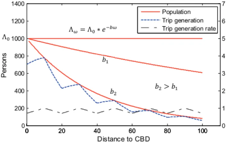
As mentioned earlier, we investigate the influence of population density on TNDP. To this end and for simplicity of illustration, we adopt the density saturation gradient model to represent the evolutionary process of population density, which states that the intensity of population density declines as the distance or travel time to CBD increases.

It can be represented by the basic equation: 0

b

e Z Z

/ / , where /_Z is the population density at distance

Z

from

the city center; /0 is the density of the central business district (CBD) at the city center; bstands for the density

gradient or slope factor. In most urban areas, the higher CBD density and lower suburban density will tend to equalize over time. As shown in Fig. 1, the population density will increase from the bottom red curve to the top

horizontal line over time; that is, bwill decrease gradually. The trip generation rate in the catchment area of a

specific transit station decreases linearly with the walking distance from the station, represented by the black dashed

line, plotted on the right Y-axis. Let Zi be the coordinate of station i and ri be the radius of its catchment area. We

assume the catchment areas of stations do not overlap with each other. The trip generation rate is defined as

0 0* ,

i i i i i i

a a c Z Z Z dr Z Zd r, where a c0, 0, respectively, are the intercept and slope of the trip generation

rate function. The total trips generated at station i for a linear network is calculated by

0 0 0 0 0 0 i i i i i i i i i i r r _b _b i _r i i _r i P Z Z a d Z Z a c e dZ Z Z a c e dZ Z Z Z Z Z Z Z Z Z Z Z Z Z Z / ª¬ ¼º/ ª¬ ¼º/

³

(1)

The blue dotted line represents the trips generated along the transit line when a0 1,c0 0.03. It is formulated as

(4)

Fig. 1. Population density evolution process

For the target year, the population density line is specified by the basic equation. The total trip production Pi

from zone i thus can be calculated by substituting

Z

_i, ,r a_i _iinto Equation (1). With production Pi known, we obtain

the OD demands by the gravity distribution model, expressed as qij P I Fi

j ij

¦

ZI FZ iZ

,where qij stands for the

amount of trips from zone i to j; Ij is the attractiveness for zone j, which exponentially decreases with its

distance to CBD, i.e., =100 i CBD

j

I eZ Z _;

ij

F is the travel cost friction factor that represents impedance to make trips

of various distances and is set proportional to the distance between two stations lij. In this way, through the trip

generation model (1) and gravity distribution model described above, we obtain the expected OD demand. In this paper, we take the planning horizon as the morning peak hour within a period (e.g., a year). To simplify the notation,

we use d to represent a specific OD pair instead of ij in the following. The OD demand, _Qd_{, fluctuates from day}

to day with the mean _qd

or qij:

d d

Q U and (_{E Q}d) _qd

. Let _Dd

be the destination node of OD pair d. Ud is

known as the uncertainty set in robust optimization. Let

T

be the uncertainty level. In particular, a polyhedral

uncertainty set is defined as:

^: ` : , , where (1 ), (1 ) d d d d d d d d d d d d j d d D j Q U Q q Q q Q B q q T q q T ½ ° ° {® d d d ¾ ° ° ¯

¦

¿ (2)

The polyhedral uncertainty set is less conservative than the box uncertainty set as it includes the joint constraint { : d } d _j

d d D j Q B

d

¦

(Ben-Tal et al., 2011), which is more realistic as it limits the total travelers heading for the same

destination j by an upper bound Bj. For instance, the total demand arriving at a city center is limited by the

amount of jobs, amount of retail shops or parking, etc. The essence of robust optimization is to find a sub-optimal solution for the RTL alignment as well as DAR services deployment such that the solutions are feasible even for the worst case scenario.

Problem setting 2.2.

Let G N A( , ) be the candidate transportation network with a node set N and an arc set A. A is the set of

feasible arcs ( , )i j Alinking stations i and j for i j N i, , z j. Each feasible arc ( , )i j is associated with a link

distancel_ij. DAR services use the same road network as that of RTL. To integrate the two services into one

multi-modal network, we segregate each node into three sub-nodes, namely, station sub-node, RTL sub-node and DAR

sub-node, with their corresponding set denoted as N N_s, _RTL,N_DAR. These three types of sub nodes are interconnected

with each other, allowing for passenger boarding, alighting and transferring between the two modes. OD demands are loaded or unloaded from the station sub-nodes. The RTL (DAR) sub nodes are connected by RTL (DAR) arcs.

The feasible arc set A can thus be separated into two subsets accordingly, RTL arc set ARTL and DAR arc set ADAR.

0 20 40 60 80 100 0 1 2 3 4 5 6 7 0 20 40 60 80 100 0 200 400 600 800 1000 1200 1400 Distance to CBD Pe rso ns Population Trip generation Trip generation rate Ȧఠൌ Ȧ଴כ ݁ି௕ఠ

ܾଵ

ܾଶ൐ ܾଵ Ȧ଴

(5)

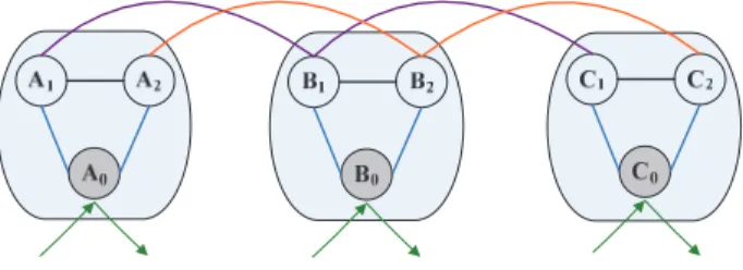
Fig. 2. Multi-modal network representation

Fig. 2 illustrates the multi-modal network with a three station network. A B C0, 0, 0 represent station sub-nodes;

1, ,1 1

A B C represent RTL sub-nodes; and A B C2, ,2 2 represent DAR sub-nodes. The purple (orange) arcs connecting 1, ,1 1

A B C (A B C2, ,2 2) are RTL (DAR) arcs, and the flows on them represent the amounts of passengers taking RTL

(DAR) services. The problem is to determine a set of RTL routes r R and their corresponding frequencies frf

as well as the deployment of DAR services to meet the stochastic OD demands so that the total expected cost is

minimized. The maximum number of lines Rmax is predefined. To select the origin and destination station for each

transit route flexibly, we introduce a dummy starting node set S { ,S r R_r } and ending node set T { ,T r R_r } so

that every RTL route r has a fixed dummy origin Sr and destination Tr. The exposition of this network structure

formulation can be found in An and Lo (2014a). For brevity and page limitation here, we skip the details and only mention the assumptions for this multi-modal problem:

(a) Each route serves both directions with the same frequency.

(b) DAR services operate on the existing road network, with congestion modeled by the BPR function. (c) Passengers can transfer between these two modes.

Assumption (a) is a common practice. (b) is how DAR services operate, serving as shuttles to carry the demands not covered by RTL. Meanwhile, they can also serve as another mode for certain congested RTL sections to mitigate crowdedness or as additional segment capacity. The road network for DAR is the same as the candidate network for RTL. The impact of private vehicles on the road network is considered directly through deducting road link capacity by their background traffic flow. The UE principle is upheld while including the congestion of DAR services. While (c) may be a simplification, we can impose a sufficient large penalty for passenger transfers between RTL and DAR so as to limit the number of transfers as in Lo et al (2003, 2004).

The decision variables are as follows. A binary variable set { }r

ij

Y

Y , ij A RTL denotes whether a link is on a

RTL. r

ij

Y is 1 if link ( , )i j is on line r; 0 otherwise. f

_{^ `}

fr stands for the RTL route frequency. The binary

variable set W

_{^ `}

W_i , i N RTL indicates whether station i is on a RTL.

d ij

X , ij A RTL, represents the passenger

flow on RTL from station i to j for OD pair d whose set is denoted as X . d

ij

Z , ij A _DAR , represents the

passenger flow on DAR from station i to j for OD pair d, whose set is denoted as Z. Vistands for the amount

of passengers transferring from RTL to DAR at station i, whereas Vistands for the amount of passengers

transferring from DAR to RTL. The transfer passenger flow set is denoted by V. Note that the first two decision

variables have directions. The problem is to determine each transit line for the forward direction, with services for the backward direction included automatically.

A robust formulation with equilibrium constraints 2.3.

The goal of the study is to minimize the system cost under the worst case scenario through locating the RTL stations, deciding the line frequencies as well as introducing DAR services as needed. To the company, these two services have different unit costs. To passengers, crowding discomfort on RTL and road congestion of DAR services are considered simultaneously to achieve a UE passenger distribution between these two modes. The network design problem with stochastic demand under UE can be formulated as a robust bi-level program, where the network

design variables

_^

Y, f, W, Z

_`

are determined in the upper level, and the UE passenger flows

_^

X, V

_`

in the lower

level. The UE principle can be represented by variational inequality (VI) constraints to reduce the bi-level problem into a single level problem with equilibrium constraints. We formulate the robust TNDP with equilibrium constraints

(6)

in P1. Let N N_RTL S T be the set of all RTL nodes including the dummy origin and destination nodes and A be the set of all RTL links including the dummy arcs. Since passenger flows on RTL, DAR or transfer links are

represented by different variables d d d, d

ij ij i i

X ,Z ,V V , it is redundant to specify the sub-node set that the subscripts of ,

d d d d

ij ij i i

X ,Z ,V V belong to. Namely, for d ij

X we must have ,i j N RTL and for

d ij

Z , we must have ,i j N DAR. To

simplify the notation, we simply use N to represent the station index without specifying the specific mode the flow

variables d d d, d ij ij i i X ,Z ,V V belong to. (P1)

1 2 3 4 5 5 5 0 min + RTL RTL DAR RTL DAR r r d ij r ij ij ij i ij ij r R ij A i N d D ij A d d d d ij ij ij ij i i d D ij A d D ij A d D i N c l f Y c l Y c W c l Z c t X c t Z c t V V

¦ ¦

¦

¦ ¦

f,Y,W,X,Z,V (3) s.t. 1, r ij RTL r R j N Y i N S d

¦¦

(4) 1, r ji RTL r R j N Y i N T d

¦¦

(5) , , r r ik kj RTL i N j N Y Y r R k N

¦

(6)

r r

1, ij ji RTL r R Y Y ij A d

¦

(7) min r max, f d f d f r R (8) 0 or 1, , r ij RTL Y r R ij A (9) max 1 0, 0 or 1, 2 r r i ij ji i RTL r Rj N r Rj N W Y Y W i N R § · ¨ ¸t ©

¦¦

¹ (10) , if d d d d kj kj j N j N X Z Q k O t

¦

(11) , if =D d d d d ik ik i N i N X Z Q k t

¦

(12) 0, D d d d d d d kj ik k k j N i N X X V V k O or z

¦

, _{k N d D Q}, , d _Ud (13) 0, D d d d d d d kj ik k k j N i N Z Z V V k O or z

¦

(14) 2 0 _{1 0.1} _, d ij d ij ij r RTL r ij X t t ij A f Y [ H § _§ _· · ¨ _¨ _¸ ¸ ¨ _¨ _¸ ¸ ¨ ¸ ¨ ¸ © ¹ © ¹

¦

(15) 4 0 _{1 0.15} _, d ij d ij ij DAR ij Z t t ij A C § _§ _· · ¨ _¨ _¸ ¸ ¨ _¨ _¸ ¸ ¨ ¸ ¨ _© _¹ ¸ © ¹

¦

(16)

DAR 0 *( ) + *( ) *( ) 0, , , RTL ij ij ij i ij i ij ij ij ij i ij A ij A i N t x x t z z t v v x z v d :

¦

₍₁₇₎ d ij ij d x

_¦

X , d ij ij d z

_¦

Z ,

d d

i i i d v

¦

V V (18) 1_{, , , ,}2 3 4 5

c c c c c are, respectively, the coefficients for RTL operating cost, RTL construction cost, station

construction cost, DAR operating cost and passenger value of time. _t0_{denotes the transfer penalty which is a}

(7)

function is to minimize the combined RTL operating cost, RTL construction cost, RTL station construction cost,

DAR operating cost and passenger cost in order to serve the random demand _Qd _Ud

. The RTL connectivity is

represented by constraints (4)-(10). Constraints (4) and (5) indicate that only one RTL sub-node is directly

connected to RTL sub-node i from upstream and downstream, respectively, if i is on route r. Constraints (4) and

(5) also ensure that at most one RTL link can be generated from the dummy origin Sr and ended at destination Tr.

Constraint (6) states that there are exactly two RTL links connecting each RTL node on route r. Constraint (7) represents that one link can be occupied by at most one transit line. Constraint (8) sets the frequency boundaries. Constraint (10) ensures that a station is constructed if any line passes through it. The first summation is the total

number of outgoing lines of station i and the second summation is the number of incoming lines. The expression in

the parentheses calculates the total number of links traversing station i, which is no more than two times the

maximum route number R_max. Wi 1 when there is a line passing through station i, and 0 otherwise. Constraints

(11)-(14) represent the passenger flow balancing conditions. The demand _Qd_{in (11)-(14) is stochastic and bounded}

by the uncertainty set _Ud_._Qd _Ud

requires that the optimal solution of P1 must be feasible for any demand

realization in _Ud_{, which leads to a min-max problem, i.e. the worst case or maximum demand scenario within the}

uncertainty set. _Od and Dd _{, respectively, represent the origin or destination node index of OD pair}_d _{. To}

accommodate the approach of robust formulation, the equality constraints for origin and destination nodes are replaced by inequalities. It is easy to see it will be pushed to equality as a consequence of the optimization. The

inequality (11) states that the total amount of passengers flowing out from station keither by RTL or DAR is greater

than the demand d

Q if k is the origin of OD pair d. The second inequality (12) follows the same logic for

destination nodes. Constraints (13) and (14) are the flow conservation constraint for RTL and DAR sub nodes, respectively. (15)-(18) are standard VI constraints to achieve UE. The passenger cost on RTL is modeled as a

non-linear function (15), where 0_{, , ,}

ij ij

t t [ H, respectively, are the free flow travel time, actual in vehicle time on RTL,

vehicle capacity and a sufficient small positive number to avoid the case of infeasibility when r 0

ij

Y . The

passenger cost on DAR services is represented by the BPR function (16), where 0_{, ,}

ij ij ij

t t C are, respectively, free flow

travel time, actual in vehicle time on DAR and road link capacity. In the VI constraints, tij, the link travel times on

RTL and DAR are, respectively, calculated by (15) and (16). Link flow is calculated by adding up flows from all OD

pairs das shown in (18).x z vij_{, ,}ij i are feasible link flows on RTL, DAR, and transfer links, respectively, with their

feasible region denoted by :. The VI constraints state that for any feasible link flow

x z vij, ,ij i

:, the optimal

link flow solution

x z vij, ,ij i

must satisfy (17). We note that : is shaped by linear constraints (11)-(14) with

stochastic demand _Qd_{, which renders}

: a polyhedron without simple, explicit boundaries. Namely, it is difficult to

determine the boundaries and extreme points of :. To deal with this challenge, we reformulate constraints (11) and

(12) associated with the demand uncertainty set into a set of linear constraints with deterministic parameters as descripted in the next section.

2.3.1.Linearization of stochastic demand constraints

We note that P1 is a non-linear model with stochastic demand. It can be reformulated as a two-stage stochastic

program with complementary constraints to minimize the expected cost as described in Lo et al. (2013) and An and Lo (2014a, 2014b). However, the problem size depends on the sample size needed to conduct the stage-two cost expectation, which limits its application for large networks. In this study, we turn to robust optimization which

focuses on the worst case scenario. For stochastic demand described by a polyhedral uncertainty set as in (2), P1 can

be linearized by reformulating the constraints related to the stochastic demand as a LP via its dual problem. The worst case scenario (highest demand combination) associated with constraints (11) and (12) are equivalent to find

the maximum _Qd_in_Ud

, which still satisfies (11) and (12): max_d d Q Q , ^: ` . . , , d d _d d d d j d d D j s t Q q Q q Q B d d

_¦

d (19)

We rewrite the polyhedral uncertainty set _Ud

, i.e. the constraints in (19), as AQddb for simplicity, where

^

`

^

_Qd,_d _{d D}: d _j

`

d

Q is the vector of d

Q involved in _Ud_;

(8)

and the RHS vector of the linear constraints. An equivalent constraint can be obtained by its dual problem (Ben-Tal et al., 2011, Bertsimas and Sim, 2004).

max_d d . . Q Q s t d d AQ b min_d T d s t. . T d 1, dt0 Ȝ b Ȝ A Ȝ Ȝ (20) where

^

₁_d, ₂_d, ₃_Dd

`

O O O d

Ȝ is the vector of dual variables corresponding to the three constraints in (19), and_Dd_is

the destination node index of OD pair d. The constraint objective of (11) changes from finding the maximum Qd

that is less than d d, if d

kj kj

j N X j N Z k O

¦

to finding the minimum _bT d

Ȝ that is less than

, if

d d d

kj kj

j N X j N Z k O

¦

. Constraint (12) follows the same logic. It enables us to directly add the dual problem

to P1 as constraints. By applying this method, constraints (11) and (12) are replaced by:

1 2 3 , is the origin of OD , d d d _d d d D d d kj kj D j N j N q q B X Z k d d O O O d

_¦

(21) 1 2 3 , is the destination of OD d, d d d _d d d D d d ik ik D i N i N q q B X Z k d O O O d

_¦

(22) 1 2 3 1, d d d d D D B d O O O (23) 1 2 3 0, d d d D _d

O

ˈ ˈ

O

t (24)

After the linearization, the feasible passenger flow set : is shaped by a set of linear constraints (13), (14) and

(21)-(24). Now : is a bounded polyhedron with finite vertexes. This attribute of : will assist us in developing

efficient solution algorithm.

2.3.2.Linearization of the VI constraint

In the VI constraint, we seek to find passenger link flow x ,z ,v_ij _ij _i so that for any feasible flow

x z vij, ,ij i

:,

(17) is satisfied. However, it is computationally formidable to enumerate all the feasible flows in :. Since : is a

bounded polyhedron, the feasible flows can be calculated by the convex combination of the vertices or extreme

points of :. Take xijfor example, xij

¦

_eK_exij e,,

¦

_eK_e 1, 0dK_ed1, where xij e, represents the eth extreme point

or vertex of :. Let zij e, andvebe defined in the same way and the number of extreme points be denoted by E. For

RTL passenger flow, we have:

_, _,

_,

*( ij) *( ij e) *( ij e) *( ij e)

ij ij ij ij e ij e ij e e ij ij

e e e e

t x x t x

_¦

K x t

_¦

K x

_¦

K x

_¦

K t x x (25)

The VI constraint (17) is reformulated as: DAR 0 , , , *( ) + *( ) *( ) 0 RTL ij e ij e i e e ij ij ij ij i e ij A ij A i N t x x t z z t v v K § · d ¨ ¸ © ¹

¦

(26)

It is obvious that if the main bracket on the LHS of (26) is less than or equal to zero for any e 1...E, then (26)

must hold. (17) is equivalent to the following constraints:

DAR 0 , , , *( ) + *( ) *( ) 0, 1,..., RTL ij e ij e i e ij ij ij ij i ij A ij A i N t x x t z z t v v e E d

¦

₍₂₇₎

After the reformulation, we only need to ensure the feasibility of (27) for all extreme points of : instead of all

(9)

problem P1. Note that P1 is a mixed integer non-linear program, with all its nonlinear terms involved in the objective function and the VI constraints. The following section describes the procedure to linearize the nonlinear terms. 2.3.2.1.Linearization of r r ij f Y A real variable r ij

y is introduced to replace the product of frequency fr and RTL construction variable Yijr, i.e.

r r

ij r ij

y f Y . r ij

y can be interpreted as the RTL link frequency which is 0 when the link is not coved by RTL and equal

to fr when a line r traverses it. A set of mixed integer linear constraints are employed to realize the transformation.

r 0 ij r y f d , r r 0 ij ij y YY d ,

r 1

r 0 ij ij r Y y f Y d , r 0 ij

y t , where

Y

is an extremely large positive number (28)

2.3.2.2.Linearization of tij and tij*zijon dial-a-ride services, ij A DAR

A continuous real variable tijis introduced to represent the total passenger travel time on link ij using DAR

services, i.e., tij t_ij*z_ij. The link travel time t_ij and total travel time tij only depend on link flow z_ij. We adopt a

piecewise linear function to approximate the nonlinear functions of t_ij and tij. The idea is to partition the passenger

flow z_ij into segments first. The passenger flows at the breaking points are denoted as m, 0,...,

ij

z m . The link

travel time m

ij

t and total link travel time tijm at breaking points are obtained through plugging z_ijm into the

corresponding travel time functions. The arc between two break points is approximated by a straight line connecting

the two adjacent breaking points, with the slope of m m1 m m1

ij ij ij ij t t z z _for ij t function and m m1 m m1 ij ij _ij _ij t t z z _for ij t

function. Now we are ready to formulate the piecewise linear functions for each link ij A DAR:

1 1 0 0 1 1 1 1 , m m m m ij ij ij ij m m ij ij ij ij m m ij m m ij m ij ij m ij ij t t t t t t t t z z P z z P

¦

(29) 1 m ij ij m z

_¦

P (30)

m m1

_* m m

m m1

_* m1_, _1,..., ij ij ij ij ij ij ij z z N _dP _d z z N m ₍₃₁₎ 0, 1,..., m ij m P t ; 0 _1, _0, m

_{^ `}

_{0,1 ,} _1,..., ₁ ij ij ij m N N N ₍₃₂₎ m ij

P is the length of the segment m covered by z_ij. For instance, if z_ijfalls in the kth_segment, m

ij

P is equal to

the length of the segment for 1dm kd 1, i.e. m m m1

ij zij zij

P _{, and is less than the length of the last segment, i.e.}

1

m m m

ij zij zij

P _d _for_{m k}_{. For}_k_d₁ _m_d_, m ₀

ij

P . This segment scheme is ensured by constraints (30)-(32).

The piecewise linear functions for tij and tij are represented by (29).

2.3.2.3.Linearization of t and ij tij*x on rapid transit services, ij ij A RTL

The RTL link travel time function is more complicated than that of DAR services since it involves two variables,

link capacity * r*

r ij rf Y [

¦

and link flowxij. This two-dimensional function requires a different approximation

method. We make use of the same piecewise linear approximation method for multi-dimensional functions as

described in Luathep et al. (2011). Similarly, the total travel time on link ij through rapid transit services is denoted

by tij t_ij*x_ij. The link capacity is denoted by y_ij

¦

_r f_r*Y_ijr*[ H . x_ij is segmented intointervals while y_ij

is segmented into `intervals. They partition the domain into *` rectangles. Each rectangle can be further

separated into two triangles by the upward diagonal line. The feasible domain of t_ij and tijis thus partitioned into a

(10)

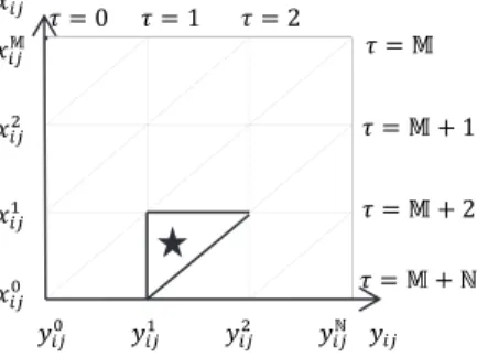
Fig. 3. Piecewise linear approximation for two dimensional functions

The key issue is to determine the active triangle that

x y_ij, _ij

falls into. Let

m_, n_, m n, _, m n,

ij ij ij ij

x y t t be the coordinate

of an arbitrary corner point

m n,

, 0 dmd,0d dn `. tij and tij are represented by the convex combination

of the corner point coordinates of the active triangle. Special ordered sets (SOS) variables are introduced in

constraints (35)-(41) to identify the active triangle that

x yij, ij

belongs to.

^ `

Dijm , m 0,..., and

^ `

n , 0,...,

ij n

E ` are Special Ordered Set of type One (SOS1) variables, which require that at most one member

from the set may be non-zero. SOS1 variable is to represent a set of mutually exclusive alternatives.

^ `

JijW , W 0,..., , +1, ...,`is Special Ordered Set of type Two (SOS2) variables, which requires that at most

two adjacent members from the set are non-zeroes. , , 0 0 0 0 , n m n m m n ij ij ij ij ij ij m n m n x

_¦¦

G x y

_¦¦

G y ` ` (33) , , , , 0 0 0 0 , m n m n m n m n ij ij ij ij ij ij m n m n t

_¦¦

`G t t

_¦¦

` G t (34) , 0 0 1 m n ij m n G

¦¦

` , m n,

_{> @}

_{0,1 ,} _{0,..., ,} _0,..., ij m n G ` (35) , 1 0 , 0,..., m n m m ij ij ij n m G _dD D

¦

` (36)

> @

0 1 _0, m _{0,1 ,} m _1, _1,..., ij ij ij ij SOS m D D D D ₍₃₇₎ , 1 0 , 0,..., m n n n ij ij ij m n G _dE E

¦

` (38)

> @

0 1 _0, n _{0,1 ,} n _1, _1,..., ij ij ij ij SOS n E E` E E _`₍₃₉₎ , 0 , 2, 0,..., , 1,..., m m ij ij ij m SOS W W W J G J W

¦

` _,_{max 0,}

_^

_W

_`

_d_m_d_min

_^

_`_W_,

_`

₍₄₀₎ 0 1 ij W W J

¦

` (41) Proposition 1: A feasible solution for the SOS1 and SOS2 variables identifies a unique triangle in the domain of

x y_ij, _ij

.

Proof: Without loss of generality, 1

ij

D , 2

ij

E are assumed to be the positive elements in SOS1 set of variables.

Substitute the values of SOS1 variables into constraints (36) and (38), we obtain

, , , 0, 1 1, 1 0 0 0 0, 2,3,..., m n n n ij ij ij ij ij n n n m G G dD G dD

¦

`

¦

`

¦

` (42) ݕ௜௝଴ ݕ௜௝ଵ ݕ௜௝ଶ ݕ௜௝Գ ݕ௜௝ ߬ ൌ ॸ ൅ ͳ ߬ ൌ ॸ ൅ ʹ ߬ ൌ ॸ ൅ Գ ߬ ൌ ॸ ݔ௜௝ ݔ௜௝ॸ ݔ௜௝ଶ ݔ௜௝ଵ ݔ௜௝଴ ߬ ൌ Ͳ ߬ ൌ ͳ ߬ ൌ ʹ

(11)

, , ,1 2 ,2 2 0 0 0 0, 0,3, 4,..., , m n m m ij ij ij ij ij m m m n G G dE G dE

¦

`

¦

(43) Combining (42) and (43), we can get

0,1 0,2 1_, 1,1 1,2 1

ij ij ij ij ij ij

G G dD G G dD , 0,1 1,1 2_, 0,2 1,2 2

ij ij ij ij ij ij

G G dE G G dE (44)

All the other m n,

ij

G which are not stated in (44) are zero.

,

m n ij

G takes on a positive value only at the corner point of the rectangle

The active rectangle is thus determined by the two sets of SOS1 variables. The next question is whether the SOS2

variable ij

W

J can identify the active triangle. In constraint (40), ij

W

J is defined as the sum of m n,

ij

G along each diagonal

line. Hence the nonzero JijW can only occur at the three possible diagonal lines, W ,W 1,W 2, passing

through points (1,1), (0,1) & (1,2), and (0,2), respectively, as shown in Fig. 3. It is easy to show that the two feasible

solutions _, 1 ₀

ij ij

J J _! _{, or} 1_, 2 ₀

ij ij

J J _! _{identify the upper and lower triangle, respectively. This finishes the proof.}

Reversely speaking, to determine the target point as shown in Fig. 3, the positive elements in SOS1 and SOS2

variables can only be 1

ij D , 2 ij E , Jij, 1 ij

J _{while all the other elements are zero.}

After the reformulation, the original robust optimization problem with equilibrium constraints is reduced into a mixed integer linear problem (MILP) which can be readily solved. The equivalent MILP is summarized as follows:

(P2) _min

1 2

3 4 5 ₊ 5 5 0 RTL RTL DAR RTL DAR r r ij ij ij ij ij ij i ij ij i r R ij A i N ij A ij A ij A i N c l y c l Y c W c l z c t c t c t v

¦ ¦

¦

f,Y,W,X,Z,V (45) s.t.

RTL connectivity constraints: (4)-(10) and (28) (46)

Passenger flow conservation constraints k N d, D: (13), (14), (18), (21)-(24) (47)

Linear constraints for link ij A DAR: (29)-(32) (48)

Linear constraints for link ij A _RTL: (33)-(41) (49)

The VI constraint: (27) (50)

Note that as a MILP, the solution directly obtained in this reformulation actually achieves global optimality, subject to the accuracy of the discretization scheme adopted here.

Solution algorithm 2.4.

P2 is a MILP and can be readily solved by a solver such as CPLEX. Nevertheless, the number of extreme points

constituting constraint (50) could be huge, which makes P2 often too large to be handled by a commercial solver.

Instead, we adopt the cutting constraint algorithm (CCA) to add the extremely points iteratively. The VI constraint

for one extreme point of the feasible region : is added into P2 one at a time. This approach substantially decreases

the initial scale of P2 and will shorten the searching time for optimal solution. When a new VI constraint for another

extreme point is included, the solver makes use of the current solution as a starting point which greatly expedites the

searching process. The relaxed MILP with a reduced number of extreme pointsEi,E Eid is formulated as:

(P3) _min

1 2

3 4 5 ₊ 5 5 0 RTL RTL DAR RTL DAR r r ij ij ij ij ij ij i ij ij i r R ij A i N ij A ij A ij A i N c l y c l Y c W c l z c t c t c t v

¦ ¦

¦

f,Y,W,X,Z,V (51) s.t. (46)-(49) and i DAR 0 , , , ( * ) + ( * ) *( ) 0, 1,..., RTL ij e ij _ij ij e ij _ij _i i e ij A ij A i N t t x t t z t v v e E d

¦

₍₅₂₎

(12)

extreme points. Additional extreme points can be found by identifying any feasible solution

x ,z ,vij ij i

: that satisfies DAR * _* * _* ₀ _* ( * ) + ( * ) *( ) 0 RTL ij ij ij ij ij ij i i ij A t t x ij A t t z i N t v v !

¦

(Luathep et al., 2011). Adding this extreme

point into P3 will make the current optimal solution infeasible, which thus leads to a new solution. An equivalent

optimization problem P4 is formulated to find the extreme points:

(P4) DAR * _* * _* ₀ _* max ( * ) + ( * ) *( ) RTL ij _ij _ij ij _ij _ij _i _i ij A ij A i N F t t x t t z t v v

¦

X,Z,V (53) s.t. (47)

If F!0, its optimal solution

x ,z ,vij ij i

will formulate a new VI constraint (50) which is then added into P3.

Otherwise we can claim that the global optimal solution for P2 has been found.

After solving P2, the line alignment and frequency of rapid transit lines _{f , Y , W}* * *_{are fixed for the whole}

studying horizon (say, a year). Moreover, P2 also calculates the DAR services needed under the worst-case (or

highest) demand scenario. The exact deployment of dial-a-ride services for a particular day will depend on the demand realization. Meanwhile, the passenger cost under UE will change with demand as well. We calculate the average DAR operating and passenger costs by drawing samples of the uncertain demand. With the RTL capacity

fixed by _{f , Y , W}* * *_{, for a specific demand realization,}_P2_{is reduced to a traditional UE traffic assignment problem.}

A variety of efficient solution approaches, such as Frank-Wolfe algorithm, Gradient Projection algorithm, etc. (Chen et al., 2002) can be applied. We adopt the Frank-Wolfe algorithm in this paper. The procedure is summarized as follows:

Step 0. Define the boundaries of the study area, location of CBD, initial population density in CBD, and population density evolutionary pattern over time.

Step 1. Determine the population in the catchment area of each candidate transit station. For a specific year, the

density distribution pattern is determined by 0

b

e Z Z

/ / . Given a candidate transit network topology (say, a linear network with a certain number of nodes), the study area could be partitioned into a set of disjoint segments according to the walking distance to the candidate transit station. Each segment is defined as the catchment area of the candidate station and the total population resided in the catchment area can be

calculated by integrating /_Zover distance

Z

.

Step 2. Determine the OD demand matrix. The total trip amount P_i generated in the predefined catchment area is

calculated by integrating the product function of population and trip generation rate over distance

Z

as

shown in (1). Trip distribution is conducted by the gravity model d

ij i j ij i

q q P I F

_¦

_ZI F_Z _Z to obtain the expected OD demand matrix.

Step 3. Determine the uncertainty level

T

of stochastic demand _Qd_{and formulate the MILP problem}_P3_without

the VI constraint (52). Namely, the system optimal solution is adopted as the initial solution.

Step 4. Solve the relaxed MILP P3 with a reduced set of extreme points. The optimal solution is denoted as

* * * * * * * *

f , Y , W , t , t , x , z , v .

Step 5. Solve the linear program (LP) problem P4 for a new extreme point

x ,z ,vij ij i

:.

Step 6. Convergence check. If Fd

H

, terminate the procedure and the optimal solution under UE flows are

maintained as _{f , Y , W , t , t , x , z , v}* * * * * * * *_{. Otherwise, add}

ij ij i

x ,z ,v into P3 through the VI constraint (52) and repeat Step 4 until the convergence criteria is satisfied.

Step 7. Calculate the average passenger cost under UE by sampling the stochastic demand given the RTL network

* * *

f , Y , W .

Step 8. Decrease bto simulate the population density increase over time and repeat Steps 2-7to find the critical population density for the first financially sustainable RTL and its construction sequence over time.

3.Case study

(13)

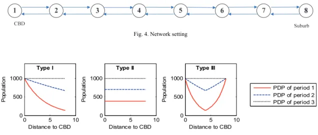
and performance, as shown in Fig. 4. The density /₀ at the city center CBD is 1000 people per km2_{. The candidate}

stations are uniformly distributed along the corridor with a distance of 1 km between two adjacent stations. There are 8*8 OD pairs in total. The inter-zonal OD trip distribution is conducted through the gravity model. In addition, we assume that the inner zonal demand can walk to their destinations and thus would not contribute to road

congestion. The trip generation rate is defined as ai 1 0.02*Z Z Z i , i d5 Z Zd i5iin Section 2.1. The robust

parameter is T 0.3 , and the trips heading for destination j is no more than 1.2 times its expectation:

^

: (1 0.3) (1 0.3), d (1 0.2) d

`

d d d d d d d d

D j D j

Q U { Q q dQ dq

_¦

Q d

_¦

q . The frequency boundaries are

max 20 /

f hr and f_min 3/hr. The transit unit capacity isC 80 persons/h. The road links has a capacity of

200

ij

C . At most 1 transit line is allowed in the network, i.e. R_max 1. The unit RTL operating cost per transit

unit is _c1 ₁_{; the unit line construction cost is}_c2 ₄_{; the unit station construction cost is}_c3 ₁_{; the unit DAR}

operating cost is proportional to the unit RTL operating cost per passenger _c4 _c1_/_[_{; the passenger value of time is}

5 _0.01

c . The transfer penalty is: _t0 ₃_{. In this study, we are interested in the critical population density that the}

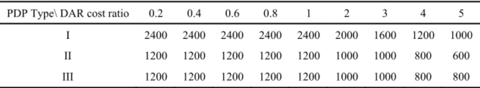
first financially sustainable RTL can be constructed and the RTL construction sequence as the population increases over time. Intuitively, many factors are influential to the RTL construction sequence, such as the population distribution pattern, the number of CBDs, and DAR services cost. In the following, sensitively analysis is employed to investigate the system performance under different combination of the influencing factors.

For a fixed population, planners decide how to spread the population density over the city, and residents decide their housing or activity locations based on their accessibility to work places, and amenities, etc. Hence, there are different population distribution patterns (PDP), such as decreasing density from CBD to the suburb as is commonly observed, uniform distribution pattern, or high density at CBD and in the suburb but low density midway between them as in certain new towns in Hong Kong. We select three representative PDPs, referred to as Type I, II, and III in Fig. 5. The solid lines show the basic shape of the population distribution and the dotted lines represent population density changes over time. The area under each curve is the total population, which can be calculated by integrating the PDP function over the X-axis. For Types I and III, the population density is represented by an exponential

function 0

b

e Z Z

/ / with the saturation density /₀ at CBD or suburb.

Z

is distance from CBD. For type II, we

define / _Z b*/₀, which is uniformly distributed along the city. b represents the degree of saturation.

Fig. 4. Network setting

Fig. 5. Population distribution pattern

Illustration of solution procedure 3.1.

Before we embark on discussing the system performance, to illustrate the formulation and solution procedure, the

solutions for the scenario of PDP Type I, with CBD located at

Z

0 and a total population of 3000 are presented

0 5 10 0 500 1000 Distance to CBD P opul at io n Type I 0 5 10 0 500 1000 Distance to CBD P opul at io n Type II 0 5 10 0 500 1000 Distance to CBD P opul at io n Type III PDP of period 1 PDP of period 2 PDP of period 3

(14)

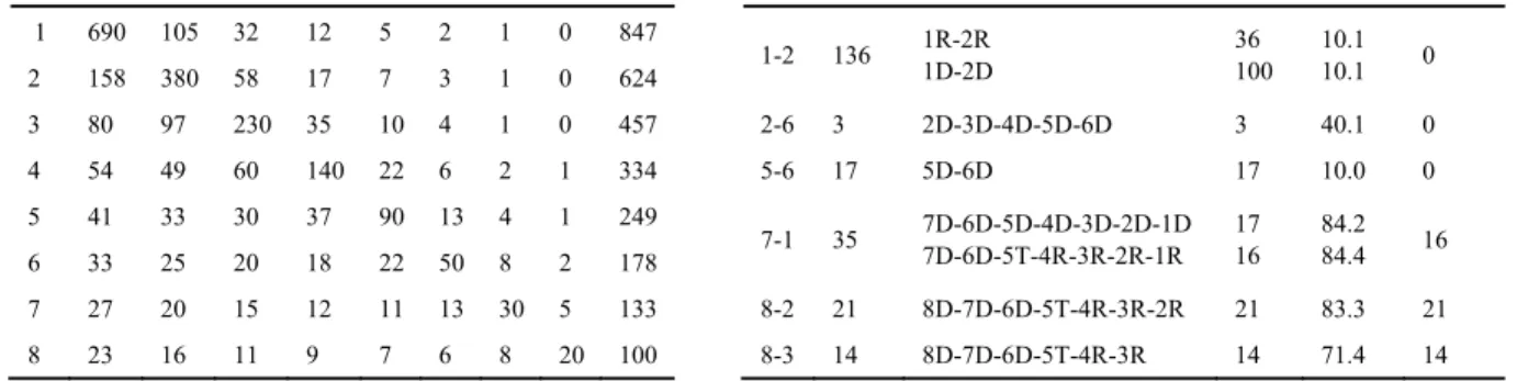
below. We first calculate the expected OD demand matrix according to Steps 2 and 3, as shown in Table 1. The last

column shows the total trips produced from each node, as calculated by (1). The amount of trip productions P_i

exponentially decreases from CBD to the suburb, i.e. from node 1 to node 8. The attractiveness of destination Ajis

expressed as an exponentially decreasing function from CBD. Now we are ready to formulate P3 with the

parameters and demand information as determined in Step 3. We repeat Steps 4-6 until the UE condition is satisfied. The algorithm took 1 to 9 iterations to converge to the UE solution. The robust solution for the worst case scenario is obtained in Step 6. With the RTL alignment, frequency and the provided DAR services fixed at the worst case scenario, we calculate the expected passenger cost in Step 7. The computational times for different scenarios vary from 9 to 151 seconds, with an average of 56 seconds.

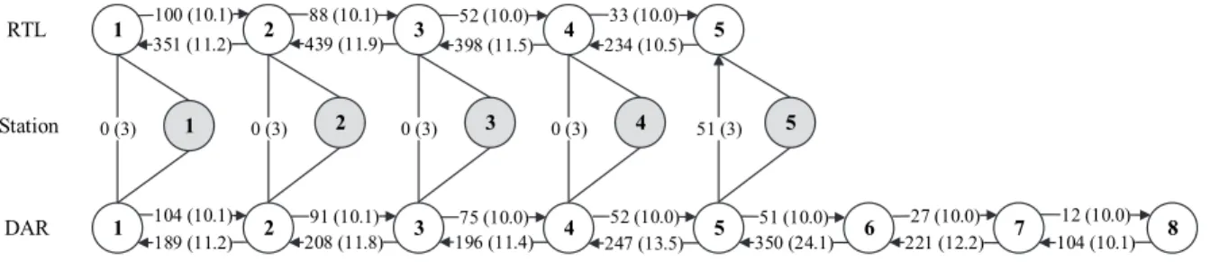
In this solution instance, the RTL services cover links from node 1 to node 5 with a frequency of 4 vehicles per hour. The resultant multi-modal network together with the link flows are shown in Fig. 6. The top nodes and links indicate the RTL services; the middle layer nodes in gray indicate station nodes where demands enter; the bottom layer nodes and links represent DAR services; and the vertical links represent transfer links between RTL and DAR with arrows indicating their directions. The figure on each link stands for the amount of passengers on specific services and the one in parenthesis for its link travel time.

To ascertain that the UE flow pattern is achieved by the cutting constraint algorithm, we depict the passenger assignment result for 6 representative OD pairs under the worst case scenario, which is sufficiently simple to track

down the details. Note that the demand for P2 under the worst case scenario shown in the second column of Table 2

is higher than the expected demand in Table 1. Column 3 in Table 2 shows the path and transport mode for each OD pair; the number stands for the node and alphabet for the transport mode, i.e. R for RTL, D for DAR, and T for Transfer. Passengers may choose different paths, and the used paths have essentially the same travel time, with a miniscule difference due to the linearization error. For OD pair 1-2, paths 1R-2R and 1D-2D have the same minimum travel time of 10.1. The unused path has longer travel time, i.e. for OD pair 2-6, the travel time on the unused path 2R-3R-4R-5T-6D is 43.1, higher than 40.1, as consistent with the UE principle. Passengers on OD 5-6 have no choice but to take DAR services since they are the only available services. We observe that most passengers choose direct services; only a few would transfer between the two modes owning to the high transfer penalty, which greatly prohibits their willingness to transfer. Table 3 shows the cost comparison between the worst case scenario and the expected cost. They have identical RTL alignment and frequencies hence have the same RTL cost. The expected cost of DAR services is 21% lower than the cost estimated by the worst case scenario, indicating that the worst case scenario overestimated the cost as expected. We anticipate that this overestimation is larger for a higher demand uncertainty. How to decide the level of demand uncertainty that the RTL services are planned for such that the expected system cost is minimized is an interesting extension to be explored in future studies.

1 104 (10.1) 2 91 (10.1) 3 75 (10.0) 4 52 (10.0) 5 51 (10.0) 6 27 (10.0) 7 221 (12.2) 350 (24.1) 247 (13.5) 196 (11.4) 208 (11.8) 189 (11.2) 8 12 (10.0) 104 (10.1) 1 100 (10.1) 2 88 (10.1) 3 52 (10.0) 4 33 (10.0) 5 234 (10.5) 398 (11.5) 439 (11.9) 351 (11.2) 0 (3) 1 0 (3) 2 0 (3) 3 0 (3) 4 51 (3) 5 RTL Station DAR

Fig. 6. RTL alignment, passenger flows and link travel time on RTL, DAR services and transfer links

Table 1. The expected OD demand qij Table 2. Path flow under UE for six representative OD pairs

O

(15)

1 690 105 32 12 5 2 1 0 847 1-2 136 1R-2R _1D-2D 36 ₁₀₀ 10.1 _10.1 0 2 158 380 58 17 7 3 1 0 624 3 80 97 230 35 10 4 1 0 457 2-6 3 2D-3D-4D-5D-6D 3 40.1 0 4 54 49 60 140 22 6 2 1 334 5-6 17 5D-6D 17 10.0 0 5 41 33 30 37 90 13 4 1 249 7-1 35 7D-6D-5D-4D-3D-2D-1D _{7D-6D-5T-4R-3R-2R-1R} 17 ₁₆ 84.2 _84.4 16 6 33 25 20 18 22 50 8 2 178 7 27 20 15 12 11 13 30 5 133 8-2 21 8D-7D-6D-5T-4R-3R-2R 21 83.3 21 8 23 16 11 9 7 6 8 20 100 8-3 14 8D-7D-6D-5T-4R-3R 14 71.4 14

Table 3 Cost component for solutions of the worst case scenario and the sample average

Alignment Freq. RTL_cost DAR_cost Passenger cost Total _cost RTL DAR Transfer Total

Worst Case 1-2-3-4-5 4 565 97 190 264 1.5 456 1118 Expectation 1-2-3-4-5 4 565 77 124 185 0 309 951 Comparison -- -- 0% 21% 35% 30% 100% 32% 15%

Sensitivity analysis of population distribution pattern (PDP) with one CBD 3.2.

In this section, only one CBD located at the origin

Z

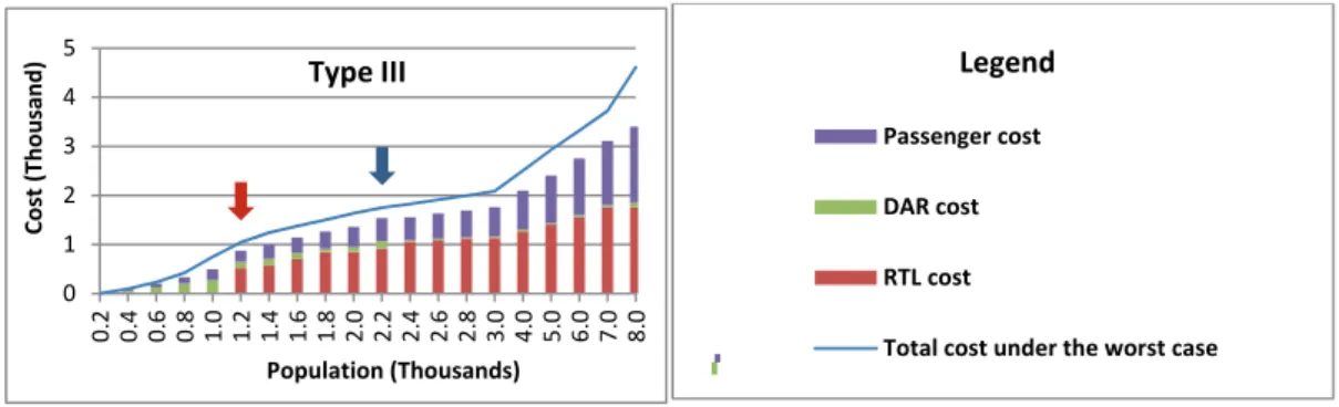
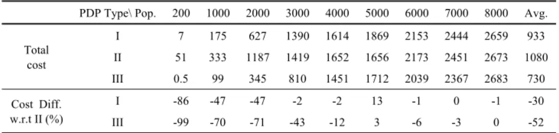
_CBD 0is considered. The RTL alignment, frequency and

cost components under the three PDPs are shown in Table 4 and Fig. 7. Twenty different population sizes varying from 200 to 8000 are tested to investigate the construction pattern of RTL over time. The step size is 200 for population ranging from 200 to 3000 and is scaled up to 1000 for population from 3000 to 8000. We can observe an obvious inflection point at population of 3000 in Fig. 7, due to the change of step size. Critical Population 1 (CP1) is defined as the population size at which the RTL is introduced for the first time whereas Critical Population 2 (CP2) is defined as the population at which the RTL is constructed to cover the whole city range. CP1 and CP2 are marked by the two arrows respectively in Fig. 7. The first RTL appears at 2400, 1200, 1200, respectively. It indicates that a dispersive population distribution will be more favorable for constructing RTL as compared with concentrating the population at CBD. CP2 for the three PDP types are 6000, 3000, and 2200, respectively. The distance between the two arrows represents the RTL construction time duration. It shows that for a uniformly distributed pattern (PDP Type II), it requires a longer time to provide RTL for the city. On the contrary, a much shorter time is needed for the

PDP dispersed to both ends. The blue curve represents the total cost under the worst scenario calculated by P3 while

the bars stand for the expected system cost calculated in Step 7 of the solution algorithm. The gap can be interpreted as the protection level offered by robust optimization to hedge against the stochastic demand. We can see that the protection level is much higher for a denser city with large population. The RTL constitutes a major cost component once introduced, whereas the DAR only constitutes a small fraction of the cost. The passenger cost linearly increases with population for the three PDP types.

0 1 2 3 4 5 0. 2 0. 4 0. 6 0. 8 1. 0 1. 2 1. 4 1. 6 1. 8 2. 0 2. 2 2. 4 2. 6 2. 8 3. 0 4. 0 5. 0 6. 0 7. 0 8. 0 Co st (Tho unds) Population(Thousands) TypeI 0 1 2 3 4 5 0. 2 0. 4 0. 6 0. 8 1. 0 1. 2 1. 4 1. 6 1. 8 2. 0 2. 2 2. 4 2. 6 2. 8 3. 0 4. 0 5. 0 6. 0 7. 0 8. 0 Co st (Tho usand) Population(Thousands) TypeII

(16)

Fig. 7. Cost component with the change of population under three PDPs and one CBD

In Table 4, we select five representative population sizes 600, 1200, 2400, 3000 and 8000 out of 20 scenarios to show the RTL alignment and cost components. The last column states the total cost comparison (%) of the three PDP types with the Type II cost selected as the benchmark. A more negative % indicates a lower cost as compared with the Type II counterpart. Type I outperforms the other types for all populations in terms of total social cost while Type III yields the highest cost. For population less than 600, the costs follow from II>III>I. When population is greater than 600 and less than 800, the rank is III>II>I. It indicates that the uniform population distribution pattern (Type II) is not beneficial to reduce total system cost for low population but will become more cost effective than concentrated development in the suburb for larger populations. The RTL capacity is enlarged to handle the increase in population either through constructing more lines or providing higher frequency. The RTL cost jump happens when a new line is constructed: i.e. for Type I, the RTL cost increases from 263 to 565 when the population changes from 2400 to 3000. In contrast, the increase in frequency does not incur that much increase in RTL cost. i.e., for Type II, the RTL cost increase from 907 to 967 when population changes from 2400 to 3000. It indicates the capital cost for line construction is the highest while operating cost increases due to increase in frequency is relatively lower. Utilization of RTL greatly reduces the use of DAR services and thus mitigates the road congestion. We can also observe that the DAR cost increases when there is no RTL, and drops dramatically when the first RTL is introduced (refer to Type I from the population of 2200 to 2400 in Fig. 7). The RTL cost, passenger cost and total cost increase with the population as expected.

As for the construction sequence, for Type I, the RTL extends gradually from CBD to the suburb; whereas for Type III, a reverse sequence is observed, i.e. from the suburb to CBD; and for Type II, the RTL starts from the middle and then expands to CBD and the suburb gradually. For Type I, the construction sequence follows the same trend as the population density increases, as expected that the RTL would be constructed on the most congested road segment first. When residents are uniformly distributed along the study area, i.e., Type II, road segments in the middle will attract most passengers. This phenomenon is incurred by the exponential distribution of the destination attractiveness to CBD from the suburb. It indicates that the demand generated from nodes 4 to 8 will head for nodes 1-3 while for the demand generated from nodes 1-3 will mostly be absolved by themselves (intra-zonal demand). Hence most OD demands have to traverse the middle road segments but not the segments at both ends. Under Type III, the high residual population in the suburb will make the road segments away from the CBD congested. Hence the construction will start from the right end nodes 4-8.

Table 4. Line alignment and the corresponding cost component with the change of total population PDP

Type Pop. RTL Alignment Freq. RTL cost DAR cost Pass. cost Total Cost Comparison (%) I 600 -- -- -- 25 15 40 -84 1200 -- -- -- 80 49 129 -82 2400* 1-2-3 3.0 263 154 211 628 -55 3000 1-2-3-4-5 4.0 565 77 309 951 -41 8000 1-2-3-4-5-6-7-8 14.0 1688 86 1579 3353 0 0 1 2 3 4 5 0. 2 0. 4 0. 6 0. 8 1. 0 1. 2 1. 4 1. 6 1. 8 2. 0 2. 2 2. 4 2. 6 2. 8 3. 0 4. 0 5. 0 6. 0 7. 0 8. 0 Co st (Tho usand) Population(Thousands)

TypeIII Legend

Passengercost DARcost RTLcost