Sobolev-Hermite versus Sobolev nonparametric density
estimation on R
Denis Belomestny, Fabienne Comte, Valentine Genon-Catalot
To cite this version:
Denis Belomestny, Fabienne Comte, Valentine Genon-Catalot. Sobolev-Hermite versus Sobolev nonparametric density estimation on R. MAP5 2016-28. 2016. <hal-01372985>
HAL Id: hal-01372985
https://hal.archives-ouvertes.fr/hal-01372985
Submitted on 28 Sep 2016
HAL is a multi-disciplinary open access archive for the deposit and dissemination of sci-entific research documents, whether they are pub-lished or not. The documents may come from teaching and research institutions in France or abroad, or from public or private research centers.
L’archive ouverte pluridisciplinaire HAL, est destin´ee au d´epˆot et `a la diffusion de documents scientifiques de niveau recherche, publi´es ou non, ´emanant des ´etablissements d’enseignement et de recherche fran¸cais ou ´etrangers, des laboratoires publics ou priv´es.
ESTIMATION ON R
D. BELOMESTNY(1), F. COMTE(2) & V. GENON-CATALOT(3)
Abstract. In this paper, our aim is to revisit the nonparametric estimation of f assuming that f is square integrable on R, by using projection estimators on a Hermite basis. These estimators are defined and studied from the point of view of their mean integrated squared error onR. A model selection method is described and proved to perform an automatic bias variance compromise. Then, we present another collection of estimators, of deconvolution type, for which we define another model selection strategy. Considering Sobolev and Sobolev-Hermite spaces, the asymptotic rates of these estimators can be computed and compared: they are mainly proved to be equivalent. However, complexity evaluations prove that the Hermite estimators have a much lower computational cost than their deconvolution (or kernel) counterparts. These results are illustrated through a small simulation study.
(1) Duisburg-Essen Universit¨at, Germany. email: [email protected]
(2)MAP5, UMR CNRS 8145, Universit´e Paris Descartes, France. email: [email protected]
(3)MAP5, UMR CNRS 8145, Universit´e Paris Descartes, France. email: [email protected].
Keywords. Complexity. Density estimation. Hermite basis. Model selection. Projection esti-mator.
Mathematics Subject Classification. 62G05-62G07.
1. Introduction
ConsiderX1, . . . , Xn n i.i.d. random variables with unknown densityf. The nonparametric
estimation off has been the subject of such a huge number of contributions in the past decades that it is difficult to make an exhaustive list of references. Roughly speaking, there are two approaches, kernel or projection method. In the projection method which is our concern here, for f belonging to L2(R), considering an orthonormal basis of this space, estimators are built by estimating a finite number of coefficients of the development of f on the basis. Fourier and wavelet bases, for instance, are commonly used. Bases of orthogonal polynomials are also used for compactly supported densities (see e.g. Donoho et al. (1996), Birg´e and Massart (2007), and Efromovich (1999), Massart (2007), Tsybakov (2009) for reference books). For densities with non compact support included inR+, recent contributions use bases composed of Laguerre functions (seee.g. Comte and Genon-Catalot (2015), Belomestnyet al. (2016), Mabon (2015)). To our knowledge, for densities onR, the use of a Hermite basis is only considered in Schwarz (1967) and Walter (1977). In this paper, our aim is to revisit the nonparametric estimation of f assuming that f ∈ L2(R) by using projection estimators on a Hermite basis. To find asymptotic rates of convergence and optimize the risk bound, authors generally assume that the unknown density belongs to a function space specifying some regularity properties off. Here, we consider the Sobolev-Hermite spaces which are naturally associated with the Hermite basis
Date: September 27, 2016.
2 D. BELOMESTNY , F. COMTE & V. GENON-CATALOT
and are defined in Bongioanni and Torrea (2006). It turns out that the Sobolev-Hermite space of regularity index sis included in the classical Sobolev space with same index. Therefore, we are led to compare the performances of the projection estimators on the Hermite basis with those of the deconvolution estimators which are projection estimators on the sine cardinal basis. Deconvolution estimators have been widely studied mainly for observations with additive noise and also for direct observations (seee.g. Comteet al. (2008)). The optimalL2-risk for density estimation on a Sobolev ball with regularity index s is of order O(n−2s/(2s+1)), see Schipper (1996), Efromovich (2008) and Efromovich (2009) For densities having a fifth-order moment belonging to a Sobolev Hermite ball with the same regularity index s, we obtain the same rate. Therefore, from the asymptotic point of view, no difference can be made between these two classes of estimators at least for non heavy tailed densities. Other examples and counter-examples are discussed.
While most papers focus on deriving minimax convergence rates, the computational efficiency of the proposed estimator is not often considered. This issue is especially important for densities with non compact support. We prove that the Hermite estimators have a much lower complexity than the deconvolution estimators, resulting in a noteworthy computational gain.
In Section 2, we present the Hermite basis, and theL2-risk of the associated projection estimators is studied together with the possible orders for the variance term. A data-driven choice of the dimension is proposed and the associated estimator is proved to be realize adequately the bias-variance tradeoff. In Section 3, results on deconvolution estimators are presented. Section 4 is devoted to the study of asymptotic rates of convergence. From this point of view, the two approaches of the previous sections are proved to be equivalent, except in some special cases. Then, we compare the complexity of the procedures and conclude that the Hermite method has a substantial advantage from this point of view. Section 5 is devoted to numerical simulation results, and aims at illustrating the previous findings. Proofs are gathered in Section 6.
2. Projection estimators on the Hermite basis.
2.1. Hermite basis. Below, we denote by k.k the L2-norm on R and by h·,·i the L2-scalar product.
The Hermite polynomial of order j is given, for j≥0, by:
Hj(x) = (−1)jex
2 dj
dxj(e− x2
).
Hermite polynomials are orthogonal with respect to the weight function e−x2
and satisfy:
R
RHj(x)Hℓ(x)e−
x2
dx = 2jj!√πδj,ℓ (see e.g. Abramowitz and Stegun (1964)). The Hermite
function of order j is given by:
(1) hj(x) =cjHj(x)e−x
2/2
, cj = 2jj!√π−1/2
The sequence (hj, j ≥0) is an orthonormal basis of L2(R). The density f to be estimated can
be developed in the Hermite basisf =Pj≥0aj(f)hj where aj(f) =RRf(x)hj(x)dx=hf, hji.
We defineSm= span(h0, h1, . . . , hm−1) the linear space generated by themfunctionsh0, . . . , hm−1
and fm=Pmj=0−1aj(f)hj the orthogonal projection off onSm.
2.2. Hermite estimator and risk bound. Consider a sample X1, . . . , Xn of i.i.d. random
variables with density f, belonging to L2(R). We define for each m ≥ 0, ˆfm = Pmj=0−1ˆajhj
a projection estimator of f, with ˆaj = n−1Pni=1hj(Xi), that is, an unbiased estimator of fm=Pjm=0−1aj(f)hj.
These estimators are considered in Schwartz (1967) and then in Walter (1977). As usual, the L2-risk is split into a variance and a square bias term. We give a more accurate rate for the variance term than in the latter papers. Indeed, we have the classical decomposition
E(kfˆm−fk2) = kf−fmk2+ mX−1 j=0 Var(ˆaj) =kf−fmk2+ 1 n mX−1 j=0 Var(hj(X1)) ≤ kf−fmk2+ Vm n , (2) where (3) Vm = Z R mX−1 j=0 h2j(x) f(x)dx=E( mX−1 j=0 h2j(X1)).
The infinite norm ofhj satisfies (see Abramowitz and Stegun (1964), Szeg¨o (1975) p.242):
(4) khjk∞≤Φ0, Φ0 ≃1,086435/π1/4 ≃0.8160.
Therefore, we have Vm ≤ Φ20m, as usual for projection density estimator, see Massart (2007),
Chapter 7. However, more precise properties of the Hermite functions provide refined bounds:
Proposition 2.1.
(i) There exists constant c such that, for any density f and for any integerm,
Vm ≤cm5/6.
(ii) IfE|X|5 <+∞, then there exists constant c′ such that for any integer m,
Vm ≤c′m1/2.
(iii) Assume that there exists K >0 with
|f(x)| ≤g(x) :=α 1
(1 +|x|)a, for |x| ≥K and α >0, a >1.
Then, there exists c′′ such that, for m large enough, Vm ≤c′′m2(aa+2+1).
Proposition 2.1 (i) shows that Vm is at most of order m5/6, a property obtained in
Wal-ter (1977). However (ii)-(iii) show that this order can be improved depending on additional assumptions on f.
In the next paragraph, we make no assumption on the regularity properties off and propose a data-driven choice of the dimension m leading to an estimator whose L2-risk automatically realizes the bias-variance trade-off in a non asymptotic way.
2.3. Model selection. For model selection, we must estimate the bias and the variance term. Define Mn={1, . . . , mn}, where mn is the largest integer such that m5n/6 ≤n/log(n) and set
(5) mˆ = arg min m∈Mn{−k ˆ fmk2+pen(d m)}, pen(d m) =κ b Vm n , Vbm= 1 n n X i=1 mX−1 j=0 h2j(Xi),
whereκ is a numerical constant. The quantity−kfˆmk2 estimates −kfmk2 =kf−fmk2− kfk2,
4 D. BELOMESTNY , F. COMTE & V. GENON-CATALOT
κΦ2
0m/n, which is the known upper bound of the variance term, where Φ0 is defined by (4).
Here, the fact that the order of Vm varies according to the assumptions on f justifies that we
rather useVbm, an unbiased estimator of Vm. We can prove the following result.
Theorem 2.1. Assume that f is bounded and that infa≤x≤bf(x) > 0 for some interval [a, b].
Then there exists κ0 such that, for κ≥κ0, the estimator fˆmˆ where mˆ is defined by (5) satisfies
E kfˆmˆ −fk2 ≤C inf m∈Mn kf −fmk2+κ Vm n +C′ n ,
where C is a numerical constant(C = 4 suits) and C′ is a constant depending on kfk ∞.
The estimator ˆfmˆ is adaptive in the sense that its risk bound achieves automatically the
bias-variance compromise, up to a negligible term of order O(1/n). It follows from the proof thatκ0 = 8 is possible. This value ofκ0 is certainly not optimal; finding the optimal theoretical
value of κ in the penalty is not an easy task, even in simple models (see for instance Birg´e and Massart (2007) in a Gaussian regression model). This is why it is standard to calibrate the value
κ in the penalty by preliminary simulations, as we do in Section 5.
Actually, the assumption infa≤x≤bf(x) > 0 is due to the fact that the proof requires the
condition
(6) ∀m≥m0, Vm ≥1, and ∀a >0,
X m∈Mn
e−a√Vm ≤A <+∞.
Condition (6) holds, as we can prove:
Proposition 2.2. If infa≤x≤bf(x)>0 for some interval[a, b], then, for m large enough,Vm ≥ c′′m1/2 where c′′ is a constant.
3. Deconvolution estimators.
As we want to compare the performances of projection estimators on the Hermite basis to those of projection estimators on the sine cardinal basis, we recall the definition of the latter estimators,
i.e. the deconvolution estimators. Let ϕ(x) = sin(πx)/(πx) which satisfies ϕ∗(t) = 1
[−π,π](t),
where ϕ∗ denotes the Fourier transform of ϕ. The functions (ϕℓ,j(x) =
√
ℓϕ(ℓx−j), j ∈ Z) constitute an orthonormal system in L2(R). The space Σℓ generated by this system is exactly
the subspace of L2(R) of functions having Fourier transforms with compact support [−πℓ, πℓ]. The orthogonal projection ¯fℓ off on Σℓ satisfies ¯fℓ∗=f∗1[−πℓ,πℓ]. Therefore,
(7) kf−f¯ℓk2= 1 2π Z |t|≥πℓ| f∗(t)|2dt.
The projection estimator feℓ off is defined by:
(8) feℓ(x) = 1 2π Z πℓ −πℓ e−itx1 n n X k=1 eitXkdt= 1 n n X k=1 sin(πℓ(Xk−x)) π(Xk−x) .
This expression corresponds to the fact that: ¯ fℓ= 1 2π Z πℓ −πℓ e−itxf∗(t)dt=X j∈Z aℓ,jϕℓ,j(x), aℓ,j =hf, ϕℓ,ji.
Contrary to ˆfm, the estimator feℓ cannot be expressed as the corresponding sum with the
es-timated coefficients ˜aℓ,j = n1Pnk=1ϕℓ,j(Xk) as this sum would be infinite and not defined. To
compute it in concrete, one can use (8) or a truncated version
e fℓ(n)(x) = X |j|≤Kn ˜ aℓ,jϕℓ,j(x), ˜aℓ,j = 1 n n X k=1 ϕℓ,j(Xk).
which creates an additional bias but is comparable to the previous Hermite estimator. We give the results forfeℓ and feℓ(n).
Proposition 3.1. The estimator feℓ satisfies
E(kfeℓ−fk2) ≤ kf −f¯ℓk2+ ℓ n.
If moreover M2=Rx2f2(x)dx <+∞, then the estimator feℓ(n) satisfies
E(kfeℓ(n)−fk2) ≤ 2kf−f¯ℓk2+ ℓ n+ 4 ℓ2(M 2+ 1) Kn .
Ifℓ≤nand Kn≥n2, the last term is of orderO(ℓ/n) and can be associated to the variance
term ℓ/n. Note that condition Kn ≥ n2 implies that the computation of a large number of
coefficients is required forfeℓ(n), for largen. In practice, we takeKn even smaller thannin order
to keep reasonable computation times.
As in the previous case, we can define a data-driven choice of the cutoff parameter ℓand build adaptive estimators: (9) ℓ˜= arg min ℓ≤n{−kfeℓk 2+ ˜κℓ n}, ℓ˜n= arg minℓ≤n{−kfe (n) ℓ k2+ ˜κ ℓ n},
where ˜κ is a numerical constant. Note that
kfeℓk2= 1 n2 X 1≤j,k≤n sin(πℓ(Xk−Xj)) π(Xk−Xj) , kfeℓ(n)k2 = X |j|≤Kn |˜aℓ,j|2.
We give the result for feℓ(n) only, as kfeℓ(n)k2 is faster to compute if K
n is chosen in a restricted
range,Kn≤n, see Section 4.4 and Section 5.
The following result holds.
Theorem 3.1. If Kn ≥ n2 and M2 = R x2f2(x)dx < +∞, then there exists a numerical
constant κ˜0 such that, forκ˜≥˜κ0, the estimator feℓ˜(nn) where ℓ˜n is defined by (9) satisfies
Ekfe˜(n) ℓn −fk 2≤C 1inf ℓ≤n kf −fℓk2+ ˜κ ℓ n+ ℓ(M2+ 1) n +C2 n ,
where C1 is a numerical constant and C2 is a constant depending on kfk∞.
Forfeℓ˜, an analogous risk bound may be obtained, without condition M2 <+∞ and without
the termℓ(M2+ 1)/nin the bound.
6 D. BELOMESTNY , F. COMTE & V. GENON-CATALOT
4. Comparison of rates of convergence and discussion.
In this section, we compute the rates of convergence that can be deduced from the optimization of the upper bounds of L2-risks. This requires to assess the rate of decay of the bias terms
kf−fmk2 in the Hermite case, kf−f¯ℓk2 in the deconvolution framework. The latter is usually
obtained by assuming that the unknown density f belongs to a Sobolev space. For the former, we consider the Sobolev-Hermite spaces which are naturally linked with the Hermite basis. 4.1. Sobolev and Sobolev-Hermite regularity. Fors >0, the Sobolev-Hermite space with regularity smay be defined by:
(10) Ws={f ∈L2(R),kfk2s,sobherm= X n≥0
nsa2n(f)<+∞}
wherean(f) =hf, hniis the n-th component off in the Hermite basis. We refer to Bongioanni
and Torrea (2006) for a definition using operator theory. Let F ={Pj∈Jajhj, J ⊂N, finite }
be the set of finite linear combinations of Hermite functions andCc∞the set of infinitely derivable functions with compact support. The setsC∞
c andF are dense inWs. As the Fourier transform
of hn satisfies
(11) h∗n =√2πinhn,
f ∈Ws if and only iff∗ ∈Ws. We now describe Ws when sis integer. Let
A+f =f′+xf, A−f =−f′+xf
The following result is proved in Bongioanni and Torrea (2006). For sake of clarity, we give a simplified proof.
Proposition 4.1. Forsinteger, the Sobolev-Hermite space Ws is equal to:
Ws = {f ∈L2(R), f admits derivatives up to order s,
k|fk|s,sobherm=
X
j1, . . . , jm∈ {−,+}, 1≤m≤s
kAj1. . . Ajmfk+kfk<+∞}.
Moreover, the following statements are equivalent: for sinteger,
(1) f ∈Ws,
(2) f admits derivatives up to order s which satisfy f, f′, . . . , f(s), xs−ℓf(ℓ), ℓ= 0, . . . , s−1
belong to L2(R).
The two norms kfks,sobhermand k|fk|s,sobherm are equivalent.
Now, we recall the definition of usual Sobolev spaces. The Sobolev space with regularity index
sis defined by (12) Ws={f ∈L2(R),kfk2s,sob= Z R (1 +t2s)|f∗(t)|2dt <+∞} Ifsis integer, then
Ws = {f ∈L2(R), f admits derivatives up to order s
such that k|fk|2s,sob=kfk2+kf′k2+. . .+kf(s)k2<+∞}.
The two norms k|.k|s,sob and k.ks,sob are equivalent. Therefore, for s integer, Ws ⊂ Ws.
Morevover, the following properties are proved in Bongioanni and Torrea (2006): for all s >0,
•
(13) f ∈Ws ⇒xsf ∈L2(R).
4.2. Rates of convergence. Now, we look at asymptotic rates of convergence. We first con-sider rates for Hermite projection estimators. We already studied the variance rate Vm/n (see
the bounds forVm in Proposition 2.1). If f belongs to Ws(L) ={f ∈L2(R),X
n≥0
nsa2n(f)≤L},
thenkf−fmk2 ≤Lm−s. Plugging this and the bounds of Proposition 2.1 in Inequality (2) gives
the following rates of theL2(R)-risk.
Proposition 4.2. Assume that f ∈Ws(L) and consider the three cases (i), (ii), (iii) of Propo-sition 2.1.
Case (i) (general case). For mopt= [n1/(s+(5/6))], E(kfˆmopt−fk
2).n− s s+(5/6).
Case (ii). For mopt= [n1/(s+(1/2))], E(kfˆmopt−fk
2).n− s s+1/2.
Case (iii). For mopt = [n1/(s+(a+2)/(2(a+1))], E(kfˆmopt−fk
2).n−s+(a+2)s/[2(a+1)].
Case (ii) gives the best rate. Note that the rate in case (iii) is strictly better than in case (i) as (a+ 2)/(a+ 1) < 5/3 as soon as a > 1/2. Cases (ii)−(iii) improve the results of Schwarz (1967) and Walter (1977).
Now, we can compare the rates to those of projection estimators in the sine cardinal basis. The following result is deduced from Proposition 3.1 and (7).
Proposition 4.3. If f ∈ Ws(R) = {f ∈ L2(R),kfk2
s,sob = R
R(1 +t2s)|f∗(t)|2dt ≤ R}, and
ℓopt=n1/(2s+1), we have E(kfeℓopt−fk2).n−2s/(2s+1).
If moreover Kn≥n2, E(kfeℓ(optn) −fk2).n−2s/(2s+1).
In Schipper (1996) it is proved that this rate is minimax optimal on Sobolev balls (at least for an integer s), see also Efromovich (2002) fors <1/2 and other references.
Let us compare results of Proposition 4.3 and of Proposition 4.2. AsWs⊂ Ws, see Section 4.1,
the comparison is relevant. In case (i), we see that the estimator feℓopt has a better rate than
ˆ
fmopt. In case (ii), the estimators have the same rate. In case (iii), the estimatorfeℓopt is slightly
better than ˆfmopt. In view of case (ii), the Hermite method is competitive. Indeed the moment
condition for (ii) is not very strong.
4.3. Rates of convergence in some special cases. When the densityf belongs toWsfor all s, we must obtain directly the exact rate of decay of the bias term. This is possible for centered Gaussian and some related densities as one can make an exact computation of the coefficients
aj(f). Let (14) fp,σ(x) = x 2p σ2pC 2p fσ(x) with fσ(x) = 1 σ√2π exp (− x2 2σ2) and C2p=EX 2p,
forX a standard Gaussian variable. The distribution fp,σ(x)dx is equal to εG1/2 forε a
8 D. BELOMESTNY , F. COMTE & V. GENON-CATALOT
Proposition 4.4. Assume that f =fσ. Then for mopt = [(logn)/λ] where λ= log
σ2+1 σ2−1 2 , we have E(kfˆmopt−fk 2).plogn/n.
The same result folds forf =fp,σ or any finite mixture of such distributions. We can compare
the rate of Proposition 4.4 with the rate log(n)/n, which is optimal in the class of analytical densities (see Ibragimov and Has’minskii (1980)). So the Hermite based approach outperforms the kernel method in the case of finite normal mixtures.
Forf =fσ, the estimator feℓ satisfies,
E(kfeℓ−fk2) .
1
ℓexp (−ℓ
2/2σ2) +n−1ℓ.
For ℓopt =σ√2 logn, the rate of feℓopt is
√
logn/n. The rate is identical to the one obtained in Proposition 4.4. The result is analogous forf =fp,σ.
Finally, the Cauchy density will provide a counter-example. Let
f(x) = 1
π(1 +x2).
From Proposition 2.1, case (iii), we take a= 2 and obtain for the variance term Vm . m2/3.
Using Proposition 4.1, we check that f ∈ W1, f /∈ W2. Moreover, by (13), xsf /∈ Ws for s≥3/2. Therefore, f /∈ W3/2, so the best rate we can obtain is n−s/s+(2/3) with s <3/2, for
mopt = [n1/(s+(2/3))].
For the sinus cardinale method,f∗(t) = exp (−|t|), so thatkf−fℓk.exp (−2πℓ). Therefore,
for ℓopt = logn/2π, the estimator feℓopt has a risk with rate logn/n. This is much better than
for the Hermite estimator.
This discussion on rates of convergence points out the interest of the adaptive method. Indeed, it automatically realizes the bias-variance compromise and thus the previous rates are reached without any specific knowledge onf.
4.4. Complexity. In this paragraph, we compare the Hermite and deconvolution estimators from another point of view: the computational efficiency.
Consider an estimator ˆfn of a function f whose L2-risk can be evaluated on a ball B(L) of
some functional space. Define its complexityCfˆn(ε) as the minimal cost of computing ˆfn at the
observation pointsX1, . . . , Xn, given that
sup
f∈B(L)
E(kfˆn−fk2)≤ε2.
Let us compute the complexity of the estimate feℓopt on the Sobolev ball Ws(L). As we need
to evaluate the function sin(ππℓ· ·) at all points (Xk −Xj), 1 ≤ k, j ≤ n, the cost of computing e
fℓopt is of order n2. Thus ε2 ≍ n−2s/(2s+1) yields n ≍ ε−2−1/s so that Cfeℓ
opt(ε) ≍ ε
−4−2/s as ε→ 0. So even in the case of infinitely smooth densities, the complexity of the deconvolution estimate can not be (asymptotically) lower thanε−4.A natural question is whether one can find an estimate with lower order of complexity. Note that the complexity would be the same for a kernel estimator on a ball of a Nikol’ski class with regularity s, see Tsybakov (2009), at least for kernels with a non compact support used in Ibragimov and Has’minskii (1980).
For the truncated estimator feℓ(n)
opt, the cost is of order nKn: indeed, one must compute the
estimate is competitive in term of computational cost as soon as Kn < n (however this choice
would contradict Theorem 3.1 whereKn≥n2).
Now, let us look at the projection estimator ˆfmopt for f ∈Ws(L). The cost of computing a
projection estimator ˆfm at observation points X1, . . . , Xncorresponds to the cost of computing hj(Xi) for i= 1, . . . , n and j = 0, . . . , m−1, i.e. is of ordernm. Thus we derive the following
proposition.
Proposition 4.5. Assume that f ∈ Ws(L) and consider the three cases (i), (ii), (iii) of Proposition 2.1. The the complexity of the estimate fˆmopt is given by Cfˆ(ε) ∼ ε−2−
2(α+1)
s with
α= 5/6,1/2,(a+ 2)/[2(a+ 1)], respectively.
Proof of Proposition 4.5. Taking ε2 ≍n−2s/(2s+1), hence n≍ε−2−1/s, and the three values
of mopt given Proposition 4.2 yield the result. ✷
As can be seen, the complexity order of the Hermite-based estimate ˆfmopt is lower than the
complexity order of the deconvolution estimatefeℓopt provided s > α. So in the case of densities
with finite fifth moment already for s >1/2,our approach leads to estimates with much lower complexity. The difference between the estimates ˆfmoptandfeℓopt becomes especially pronounced
in the limiting cases→ ∞,whereCfˆm
opt(ε)≍ε
−2 whileC
e
fℓopt(ε)≍ε
−4 asε→0, resulting in a
huge computational gain.
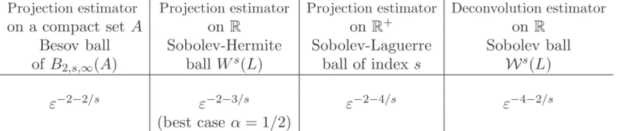
Projection estimator Projection estimator Projection estimator Deconvolution estimator
on a compact set A on R on R+ on R
Besov ball Sobolev-Hermite Sobolev-Laguerre Sobolev ball ofB2,s,∞(A) ballWs(L) ball of index s Ws(L)
ε−2−2/s ε−2−3/s ε−2−4/s ε−4−2/s
(best case α= 1/2)
Table 1. Complexity for density estimation in different contexts.
For any projection estimator, the cost of computation if of order nmopt where mopt is the
optimal dimension. In the case of a density with compact support A, if we evaluate the L2 -risk of a projection estimator on a Besov ball of B2,s,∞(A) , we have ε2 ≍ n−2s/(2s+1) with
mopt ≍n1/(2s+1), thus a cost of order ε−2−2/s, see Barron et al. (1999) for rates and definition
of Besov spaces.
In the case of a density of R+, the best L2-risk of a projection estimator on a Sobolev-Laguerre ball of indexsis of ordern−s/(s+1)withmopt ≍n1/(s+1), hence a cost of orderε−2−4/s,
see Belomestnyet al. (2016).
All these results are summarized in Table 1.
5. Simulation results
In this Section, we propose a few illustrations of the previous theoretical findings. To that aim, we consider several densities, fitting different assumptions of our setting.
10 D. BELOMESTNY , F. COMTE & V. GENON-CATALOT 0 20 40 60 80 100 0.05 0.1 0.15 0.2 0.25 0.3 0.35 0.4 0.45 0.5 0 20 40 60 80 100 0.05 0.1 0.15 0.2 0.25 0.3 0.35 0.4 0.45 0.5
Figure 1. Left: m 7→ Vbm/√m for 1 sample of densities (i) (blue line), (iv) (cyan stars), (vi) (red dashed), (ix) (green x marks) and m 7→ Vbm/m5/6 for 1
sample of densities (i) (blue dashed) and (ix) (green dash-dot). Right: the same as previously for 10 samples.
(ii) A GaussianN(0, σ2), σ= 0.5,
(iii) A mixed Gaussian density 0.4N(−3, σ2) + 0.6N(3, σ2),σ = 0.5, (iv) A Gammaγ(3,0.5) density,
(v) A mixed Gamma 0.4γ(2,1/2) + 0.6γ(16,1/4) (vi) A beta density β(3,3),
(vii) A beta density β(3,6),
(viii) Laplace densityf(x) =e−|x|/2,
(ix) A Cauchy density,f(x) = 5/[π(1 + (5x)2)].
Density (i) is proportional to the first basis function h0 and should be perfectly estimated in
the Hermite procedure, densities (vi) and (vii) are compactly supported and density (ix) does not admit any moment (in particular no fifth moment, so it does not fit case (ii) of Proposition 2.1). Hermite functions are recursively computed via (26) and with normalization (1).
We plot in Figure 1 the representation of m 7→ Vbm/√m for 1 and 10 samples drawn from
densities (i), (iv), (vi), (ix) (see (5)). It seems that the ratio is stable along the repetitions, and converges to a fixed value, which is the same in the first three cases. On the contrary,
m 7→ Vbm/m5/6 given for (i) and (ix) seems to decrease and to tend to zero in any case. It is
tempting to conclude from these plots that the order ofVm isO(m1/2) in a rather general case.
We have implemented the Hermite projection estimator ˆfmˆ with ˆm given in (5), feℓ˜(n)
n with
˜
ℓn given by (9) and the kernel estimator given by the function ksdensity of Matlab. For the
model selection steps of the first two estimators, the two constants κ and ˜κ of the procedures have been both calibrated by preliminary simulations including other densities than the ones mentioned above (to avoid overfitting): the selected values were κ = ˜κ = 4. We considered two sample sizes n= 250 andn= 1000, but as the sine cardinale procedure is rather slow, we only took K250 =K1000 = 100. The theoretical value Kn =n2 is unreachable in practice (the
computing time becomes much too large), and our choice ofKnis consistent with the complexity
considerations of Section 4.4.
Formn, we should take (n/log(n))6/5, which is of order 100 forn= 250 and 400 forn= 1000.
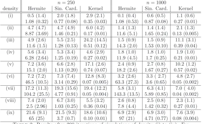
values between 0 and 10. For each distribution, we present in Table 2 the MISE computed over 200 repetitions, together with the standard deviation. In the three cases, we provide also the mean (and standard deviations in parenthesis) of the selected dimension (Hermite), cutoff (Sine cardinale) or bandwidth (kernel).
n= 250 n= 1000
density Hermite Sin. Card. Kernel Hermite Sin. Card. Kernel (i) 0.5 (1.4) 2.0 (1.8) 2.9 (2.1) 0.1 (0.4) 0.6 (0.5) 1.1 (0.6) 1.08 (0.32) 0.77 (0.08) 0.35 (0.03) 1.08 (0.53) 0.87 (0.08) 0.27 (0.01) (ii) 4.7 (4.7) 4.7 (4.9) 6.0 (4.2) 1.4 (1.3) 1.4 (1.4) 2.1 (1.3) 8.87 (3.69) 1.46 (0.21) 0.17 (0.01) 11.6 (5.1) 1.65 (0.24) 0.13 (0.005) (iii) 4.9 (2.6) 5.5 (2.5) 24.2 (14.5) 1.5 (0.9) 1.5 (0.9) 11.1 (3.1) 11.6 (1.5) 1.28 (0.13) 0.51 (0.12) 14.3 (2.0) 1.53 (0.10) 0.39 (0.04) (iv) 5.6 (3.4) 5.3 (3.4) 4.6 (2.9) 1.8 (1.0) 1.8 (1.0) 1.9 (1.0) 6.28 (2.64) 1.25 (0.19) 0.27 (0.02) 11.9 (4.5) 1.7 (0.25) 0.21 (0.01) (v) 7.2 (3.6) 6.6 (2.8) 17.1 (2.6) 2.4 (0.9) 2.7 (0.8) 10.2 (1.2) 15.1 (2.0) 1.13 (0.20) 0.74 (0.07) 18.2 (2.6) 1.67 (0.27) 0.57 (0.02) (vi) 7.2 (7.2) 7.3 (7.4) 12.8 (8.3) 3.2 (2.6) 3.3 ( 2.7) 4.8 (2.7) 46.5 (10.5) 3.14 (0.29) 0.07 (0.005) 63.3 (27.3) 3.6 (0.65) 0.05 (0.002) (vii) 17.2 (11.3) 19.3 (15.6) 19.4 (12.2) 5.8 (3.1) 6.3 (4.1) 7.0 ( 4.0) 104.2 (25.5) 4.77 (0.91) 0.05 (0.004) 143.3 (13.5) 5.89 (0.85) 0.04 (0.002) (viii) 7.4 (2.0) 6.7 (3.0) 5.5 (3.2) 2.6 (0.8) 2.5 (0.8) 2.3 (1.1) 2.5 (2.96) 1.03 (0.25) 0.36 (0.04) 7.8 (4.4) 1.42 (0.32) 0.27 (0.01) (ix) 21.6 (9.1) 21.5 (9.3) 18.6 (10.6) 6.9 (2.9) 6.9 (3.0) 7.6 (3.9) 65 (25) 3.7 (0.7) 0.10 (0.01) 97 (21) 4.71 (0.77) 0.08 (0.004) Table 2. Results after 200 iterations of simulations of density (i) to (ix). For each density (i)-(ix), first line: MISE× 1000 with (std × 1000) in parenthesis; second line: mean of selected dimension (Hermite), cutoff (sinus cardinale) or bandwidth (kernel) with std in parenthesis.
We can see from the results of Table 2 that the Hermite and sinus cardinale methods give very similar results, except for theN(0,1) where the Hermite projection is much better as expected, as the procedure most of the time chooses m = 1. The kernel method seems globally less satisfactory. The noteworthy difference between the first two methods is the computation time: as the models are nested in the Hermite projection strategy, all coefficients can be computed once for all, and then the dimension is selected. In the sinus cardinale strategy, each time ℓis changed, all the coefficients have to be recalculated. For instance, when the maximal dimension proposedmnis 50, andKnis 100, the elapsed times for 100 simulations is: forn= 250, around
0.5s for Hermite, 41s for sinus cardinale; forn= 1000, around 1.2s for Hermite, 137s for sinus cardinale, all times measured on the same personal computer to give an order of the difference. This is coherent with the lower complexity property of the Hermite method.
Table 2 also provides the selected dimensions, cutoffs and bandwidths. As could be expected, ˆ
m , ˜ℓvary in opposite way, compared to ˆh. Without surprise also, the selected dimensions and cutoffs increase when the sample size increases. What is remarkable is the values of the selected dimensions for β-distributions, which are very large. Globally, we can see that these values are very different from one distribution to the other. Contrary to the theoretical result, the Cauchy density is estimated with similar MISEs in the Hermite and sinus cardinale methods.
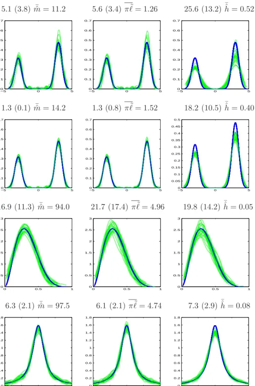
12 D. BELOMESTNY , F. COMTE & V. GENON-CATALOT 5.1 (3.8) ¯mˆ = 11.2 5.6 (3.4) πℓ˜= 1.26 25.6 (13.2)h¯ˆ = 0.52 −5 0 5 0 0.1 0.2 0.3 0.4 0.5 0.6 0.7 −5 0 5 0 0.1 0.2 0.3 0.4 0.5 0.6 0.7 −50 0 5 0.1 0.2 0.3 0.4 0.5 0.6 0.7 1.3 (0.1) ¯mˆ = 14.2 1.3 (0.8) πℓ˜= 1.52 18.2 (10.5)h¯ˆ = 0.40 −5 0 5 0 0.1 0.2 0.3 0.4 0.5 0.6 0.7 −50 0 5 0.1 0.2 0.3 0.4 0.5 0.6 0.7 −5 0 5 0 0.05 0.1 0.15 0.2 0.25 0.3 0.35 0.4 0.45 0.5 16.9 (11.3) ¯mˆ = 94.0 21.7 (17.4)πℓ˜= 4.96 19.8 (14.2) ¯ˆh= 0.05 0 0.5 1 0 0.5 1 1.5 2 2.5 3 0 0.5 1 0 0.5 1 1.5 2 2.5 3 0 0.5 1 0 0.5 1 1.5 2 2.5 3 6.3 (2.1) ¯mˆ = 97.5 6.1 (2.1) πℓ˜= 4.74 7.3 (2.9)h¯ˆ= 0.08 −1 −0.5 0 0.5 1 0 0.2 0.4 0.6 0.8 1 1.2 1.4 1.6 1.8 −1 −0.5 0 0.5 1 0 0.2 0.4 0.6 0.8 1 1.2 1.4 1.6 1.8 −1 −0.5 0 0.5 1 0 0.2 0.4 0.6 0.8 1 1.2 1.4 1.6 1.8
Figure 2. True densityf in bold blue for Model (iii) (first two lines), Model (vii) (third line) and Model (ix) (fourth line), together with 25 estimates (green/grey) withn= 250 (lines 1 and 3) or n = 1000 (lines 2 and 4). First column: Hermite; second column: Sinus Cardinale; third column: kernel. Above each plot: MISE×1000 and std×1000 in parenthesis, followed par the mean of selected dimensions, cutoffs and bandwidths (all means over the 25 samples).
In Figure (2), density and 25 estimators are plotted for models (iii), (vii) and (ix). Risks and standard deviation for the 25 curves are given above each plot, together with the mean of the selected dimension, cutoff or bandwidth. The methods are comparable, even for the Cauchy distribution, except for the mixtures, where the kernel method fails. The first two lines illustrate the improvement obtained when increasing n. We note again that the selected dimensions in the Hermite method are possibly rather high (see the beta and the Cauchy densities). However, computation time remains very short.
6. Proofs
6.1. Proof of Propositions 2.1 and 2.2. We start by proving Proposition 2.1.
(i). The following bound comes from Szeg¨o (1959, p.242) where an expression ofC∞ is given:
(15) ∀x∈R, |hj(x)| ≤C∞(j+ 1)−(1/12), j= 0,1, . . . . Therefore, (16) Vm ≤C∞2 mX−1 j=0 (j+ 1)−(1/6)≤ 6 5C 2 ∞m5/6.
(ii). Now, as in Walter (1977), we use the following expression for the Hermite function hn (see
Szeg¨o (1959, p.248)): (17) hj(x) =λjcos (2j+ 1)1/2x−jπ 2 + 1 (2j+ 1)1/2ξj(x) whereλj =|hj(0)| if j is even,λj =|h ′ j(0)|/(2j+ 1)1/2 if j is odd and ξj(x) = Z x 0 sin [(2j+ 1)1/2(x−t)]t2hj(t)dt.
By the Cauchy-Schwarz inequality,
ξj2(x)≤ Z |x| 0 t4dt Z |x| 0 h2j(t)dt≤ |x| 5 5 × 1 2. Moreover, λ2j = (2j)!1/2 2jj!π1/4, λ2j+1 =λ2j √ 2j+ 1 p 2j+ 3/2.
By the Stirling formula and its proof,λ2j ∼π−1/2j−1/4,λ2j+1 ∼π−1/2j−1/4 and for allj, there
exists constants c1, c2 such that, for allj ≥1,
c1 π1/2j1/4 ≤λj ≤ c2 π1/2j1/4. Therefore, h2j(x)≤2 c 2 2 πj1/2 + 1 2j+ 1 |x|5 5 . This yields: Z h2j(x)f(x)dx≤2 c 2 2 πj1/2 + 1 5(2j+ 1)E|X| 5, which impliesVm.m1/2.
14 D. BELOMESTNY , F. COMTE & V. GENON-CATALOT
Now we study case (iii). The following bound forhj is given in Markett (1984, p.190): There
exist positive constants C, γ, independent of x andj, such that, forJ = 2j+ 1,
|hj(x)| ≤ C(J1/3+|x2−J|)−1/4, x2 ≤2J,
≤ Cexp (−γx2), x2>2J.
Consider a sequence (aj) such that aj → +∞, aj/√j → 0 with J = 2j + 1 large enough to
ensure √aJ J ≤1/ √ 2, aJ ≥K. AsR hj2(x)dx= 1,aJ < √ J,aJ ≥K and g is decreasing, Z h2j(x)f(x)dx≤2Ckfk∞ Z aJ 0 (J1/3+J −x2)−1/2dx+g(aJ).
Setx= (J1/3+J)1/2y in the integral. This yields:
Z aJ 0 (J1/3+J−x2)−1/2dx = Z aJ/(J1/3+J)1/2 0 dy p 1−y2 = Arcsin( aJ (J1/3+J)1/2)≤2 aJ √ J.
as for 0 ≤ x ≤ 1/√2, Arcsinx ≤ 2x. Now we choose the sequence (aj) and consider aj = j1/(2(a+1)). We deduce Z h2j(x)f(x)dx.j−a/(2(a+1)), which leads to (18) Vm .m a+2 2(a+1).✷
Now we turn to the proof of Proposition 2.2 and we look at the lower bound. We have, setting
c= infa≤x≤bf(x), and using (17), Z h2j(x)f(x)dx ≥ c Z b a h2j(x)dx ≥ cλ2j Z b a cos2 (2j+ 1)1/2x−jπ 2 dx + c 2λj (2j+ 1)1/2 Z b a cos (2j+ 1)1/2x−jπ 2 ξj(x)dx. We have j−3/4c1/√π ≤ (2j+1)2λj1/2 ≤j−3/4 p 2/πc2 and | Z b a cos (2j+ 1)1/2x−jπ 2 ξj(x)dx| ≤ Z b a |x|5/2 √ 10 dx:=C.
Thus, the second term is lower bounded by −Cj−3/4c1/√π. For the first term, λ2j ≥j−1/2c21/π
and Z b a cos2 (2j+ 1)1/2x−jπ 2 dx= 1 2(b−a)+ Z b a cos2(2j+ 1)1/2x−jπdx= 1 2(b−a)+O( 1 j1/2). Therefore, Z h2j(x)f(x)dx ≥ cj−1/2c21/π b−a 2 +O( 1 j1/2) −Cj−3/4c1/√π.
6.2. Proof of Theorem 2.1. LetSm be the space spanned by{h0, . . . , hm−1} and Bm ={t∈ Sm,ktk = 1}. We have ˆfm = arg mint∈Smγn(t) where γn(t) = ktk2 −2n−1
Pn
i=1t(Xi) and
γn( ˆfm) =−kfˆmk2. Now, we write, for two functionst, s∈L2(R) , γn(t)−γn(s) =kt−fk2− ks−fk2−2νn(t−s) where νn(t) = 1 n n X i=1 [t(Xi)− ht, fi].
Then, for anym∈ Mn={1≤m≤mn},mn≤n/logn, and any fm∈Sm, γn( ˆfmˆ) +pen( ˆd m)≤γn(fm) +pen(d m). This yields kfˆmˆ −fk2 ≤ kf −fmk2+pen(d m)−pen( ˆd m) + 2νn( ˆfmˆ −fm). We use that 2νn( ˆfmˆ −fm)≤4 sup t∈Bm∨mˆ νn2(t) +1 4kfˆmˆ −fmk 2,
and some classical algebra to obtain: 1 2kfˆmˆ −fk 2 ≤ 3 2kf−fmk 2+pen(d m) + 4 sup t∈Bm∨mˆ νn2(t)−p(m∨mˆ) !
+(4p(m∨mˆ)−pen( ˆm)) + (pen( ˆm)−pen( ˆd m)).
(19)
We can choose p(m) such that
(20) X m′ ∈Mn E sup t∈Bm∨m′ νn2(t)−p(m∨m′) ! + ≤ c n.
Indeed, for this, we apply the Talagrand Inequality: E sup t∈Bm νn2(t)−4H2 + ≤ C1 n v2e−C2nH 2 v +M1 n e −C3nHM 1 where E supt∈Bmν2 n(t) ≤ Vm
n := H2, supt∈BmVar(t(X1))≤ supt∈BmE(t
2(X
1)) ≤ kfk∞ := v2
and supt∈Bmsupx|t(x)| ≤ qsupxPmj=0−1h2j(x) ≤C∞′ m5/12 ≤C∞′ √n := M1 (see (15)).
There-fore we obtain E sup t∈Bm νn2(t)−4Vm n + ≤ C1 n kfk∞e−C ′ 2Vm+√1 ne −C′ 3 √ Vm .
Therefore, with the choice p(m) = 4Vm/n, (20) holds under condition (6) which is ensured by
Proposition 2.2.
Taking expectation in (19) yields 1 2E(kfˆmˆ −fk 2) ≤ 3 2kf −fmk 2+ pen(m) +E(4p(m∨mˆ)−pen( ˆm)) +E(pen( ˆm)−pen( ˆd m))++ c n. (21) Let us define Yi(m):= mX−1 j=0 h2j(Xi), Vbm= 1 n n X i=1 Yi(m),
16 D. BELOMESTNY , F. COMTE & V. GENON-CATALOT
and the set inspired by Bernstein Inequality Ω = ( ∀m∈ Mn, 1 n n X i=1 (Yi(m)−E(Yi(m))) ≤ r 2VmC∞′′m5/6 log(n) n + 4C ′′ ∞m5/6 log(n) 3n ) .
withC∞′′ := (C∞′ )2 and C∞′ is the constant appearing inM1 above. We split the term to study
in (21) as follows:
E(pen( ˆm)−pen(d m))+≤E[(pen( ˆm)−pen(d m))+1Ω] +E[(pen( ˆm)−pen(d m))+1Ωc].
On Ω, |Vbmˆ −Vmˆ| ≤ q 2VmˆC∞′′mˆ5/6log(n)/n+ 4C∞′′mˆ5/6log(n)/(3n) ≤ 1 2Vmˆ + 7 3C ′′ ∞ ˆ m5/6log(n) n ,
using that 2xy ≤ x2 +y2 applied to √2V A = 2pV /2√A ≤ V /2 +A with V = Vmˆ and
A=C”∞mˆ5/6log(n)/n. and thus, by definition ofMn,
E[(pen( ˆm)−pen( ˆd m))+1Ω] +≤
1
2E(pen( ˆm)) +
c n.
On the other hand,
E[(pen( ˆm)−pen( ˆd m))+1Ωc]≤2κP(Ωc). Now, P(Ωc)≤ X m∈Mn 2e−2 log(n)≤ c n
as we apply Bersntein inequality: P(|Sn/n| ≥ p
2v2x/n+bx/(3n))≤2e−x forS
n=Pni=1(Ui−
E(Ui)), Var(U1) ≤v2,|Ui| ≤b. In our caseU=Yi(m) and v2 =VmC∞′′m5/6, b=C∞′′m5/6 and we
tookx= 2 log(n). So Equation (19) becomes 1 2E(kfˆmˆ −fk 2) ≤ 3 2kf −fmk 2+ pen(m) +E(4p(m∨mˆ)−pen( ˆm)) (22) +1 2E(pen( ˆm)) + c n (23) ≤ 32kf −fmk2+ pen(m) +E(4p(m∨mˆ)− 1 2pen( ˆm)) +c c n (24)
Now we note that, for κ≥8 :=κ0,
4p(m∨mˆ)−1
2pen( ˆm)≤pen(m). Finally, we get, for allm∈ Mn,
E(kfˆmˆ −fk2)≤3kf −fmk2+ 4pen(m) + c n,
6.3. Proof of Proposition 3.1. The first inequality is standard. Let us study feℓ(n)(x). We write that
kfeℓ(n)−fk2 = kfeℓ(n)−Efeℓ(n)k2+kE(feℓ(n))−fk2
≤ kfeℓ(n)−Efeℓ(n)k2+ 2kE(feℓ(n))−f¯ℓk2+ 2kf¯ℓ−fk2.
The term kf¯ℓ−fk2 is the usual bias term. moreover
E kfeℓ(n)−Efeℓ(n)k2 = X |j|≤Kn Var(˜aℓ,j) = 1 n X |j|≤Kn Var(ϕℓ,j(X1)) ≤ n1 X |j|≤Kn E[ϕ2ℓ,j(X1)]≤ ℓ n
because Pj∈Z|ϕℓ,j(x)|2 ≤ℓ. This is the standard variance term order.
The new term is
(25) kE(feℓ(n))−f¯ℓk2= X |j|≥Kn |aℓ,j|2 ≤2 sup j | jaℓ,j|2 X j>Kn j−2 ≤ 2 Kn sup j | jaℓ,j|2. We write thatjaℓ,j =j √ ℓRϕ(ℓx−j)f(x)dx=√ℓ(I1+I2) where I1 =ℓ Z xϕ(ℓx−j)f(x)dx, I2 =− Z (ℓx−j)ϕ(ℓx−j)f(x)dx
and we boundI1 and I2.
|I1| ≤ℓ sZ |ϕ(ℓx−j)|2dx Z x2f2(x)dx=√ℓpM 2, whereM2 = Z x2f2(x)dx.
On the other hand, |I2| ≤supu∈R|uϕ(u)|R f(x)dx≤1.We obtain:
|jaℓ,j| ≤ℓ p
M2+
√
ℓ≤ℓ(pM2+ 1).
Plugging this in (25), we find the bound: kE(feℓ(n))−f¯ℓk2 ≤4ℓ2(M2+1)/Kn.This term isO(ℓ/n)
if ℓ≤nand Kn≥n2. ✷
6.4. Proof of Proposition 4.1. Using the relations (see e.g. Abramowitz and Stegun (1964)) (26) 2xHn(x) =Hn+1(x) + 2nHn−1(x), Hn′(x) = 2nHn−1(x), n≥1. we get: A+hn= √ 2nhn−1, A−hn= p 2(n+ 1)hn+1. We deduce: (27) √2h′n=√n hn−1− √ n+ 1hn+1, 2x hn= p 2(n+ 1)hn+1+ √ 2n hn−1,
Assume first that f ∈ L2(R), f admits derivatives up to order s, and for j1, . . . , jm ∈ {−,+}
and 1≤ m ≤s, Aj1. . . Ajmf ∈L2(R). We prove that P
n≥0nsa2n(f) <+∞. We do the proof
only forf compactly supported and refer to Bongioanni and Torrea (2006) otherwise. For the proof, set A−1 = A−, A+1 = A+ so that, for n−j ≥ 0, Ajhn =
p 2(n+dj)hn−j, dj = 0 ifj = 1,dj = 1 if j=−1 . Thus, forn−j1−j2−. . .−jm≥0, Aj1. . . Ajmhn= q 2(n+dj1)×. . .× q 2(n+djm)hn−j1−j2−...−jm.
18 D. BELOMESTNY , F. COMTE & V. GENON-CATALOT
Now, for f compactly supported,
hAjf, hni=hf, A−jhni= q
2(n+d−j)hf, hn+ji.
Iterating yields, forn+j1+j2+. . .+jm ≥0,
hAj1. . . Ajmf, hni=hf, A−jmA−jm−1. . . A−j1hni= Y 1≤k≤m q 2(n+d−jk)hf, hn+j1+j2+...+jmi. Therefore, Pn≥0(hAj1. . . Ajmf, hni)2<+∞ is equivalent to X n+j1+j2+...+jm≥0 nma2n+j1+j2+...+jm(f)<∞.
Now assume thatPn≥0na2
n(f)<+∞.
We have f =Pn≥0an(f)hn. We can write for n1 large enough:
| nX1+n2 n=n1 an(f)hn(x)| ≤ n1X+n2 n=n1 n1+1/6a2n(f)h2n(x) nX1+n2 n=n1 n−(1+1/6) !1/2 ≤C n1X+n2 n=n1 na2n(f).
Thus, the series for f converges uniformly, f is continuous and satisfies for all x, f(x) =
P n≥0an(f)hn(x). Therefore, we have: f(y)−f(x) = X n≥0 an(f) Z y x h′n(t)dt = a0(f)(h0((x)−h0(y)) + 2−1/2 X n≥1 an(f) Z y x (√n hn−1(t)− √ n+ 1hn+1(t))dt Set SN(t) = PNn=1an(f)(√n hn−1(t)−√n+ 1hn+1(t)) and S(t) = Pn≥1an(f)(√n hn−1(t)− √
n+ 1hn+1(t)). The function S(t) is well defined by assumption and SN converges to S in
L2(R). Therefore, asN tends to infinity.
Z y
x |
SN(t)−S(t)|dt≤√y−xkSN −Sk →0.
We have proved that
f(y)−f(x) =a0(f) Z y x h′0(t)dt+ Z y x S(t)dt.
Thus,f is absolutely continuous and f′ =S belongs to L2(R). Analogously, we prove thatxf
belongs to L2(R). Thus,A+f, A−f belong toL2(R).
Next, by the same reasoning as above, using thatPnn2a
n(f)<+∞the series forf′(t) =S(t)
is uniformly convergent and f′(t) is continuous. We proceed analogously to prove that f′ is absolutely continuous and thatxf′ and f′′ belong toL2(R). Iterating the reasoning, we obtain that f admits continuous derivatives up to s−1 and that f(s−1) is absolutely continuous and that f, f′, . . . , f(s), xk−mf(k−m), m = 0, . . . , s −1 all belong to L2(R). This shows that, for
6.5. Proof of Proposition 4.4. To prove the result, we use the following proposition.
Proposition 6.1. Recall that aj(f) =R f(x)hj(x)dx. For j≥0, we have:
a2j(fσ) = c2j 1 1 +σ2 1/2 (2j)! j! σ2−1 σ2+ 1 j , a2j+1(fσ) = 0. For n≥p, j ≥0, |a2j(fp,σ)| ≤C(p, σ2)c2j (2j)! (j−p)! σ2−1 σ2+ 1 j−p , a2j+1(fp,σ) = 0.
We can now deduce the risk of ˆfm when f =fσ. We have:
a22j(fσ)∼π−1j−1/2 1 1 +σ2 σ2−1 σ2+ 1 2j .
Therefore, settingλ= logσσ22+1−1
2
yieldskf−fmk2 . √1mexp (−λm).Combining with
Propo-sition 2.1, we obtain E(kfˆm−fk2). √1mexp (−λm) +n−1√m, and thus Proposition 4.4. ✷
Proof of Proposition 6.1. We first compute the coefficients of the centered Gaussian density. As Hermite polynomials of odd index are odd, the coefficients with odd index are null. We compute the coefficients with even index. Let
(28) σ¯2= (1 +σ−2)−1 = σ
2
1 +σ2.
Note that if 2¯σ2 = 1,i.e. σ2 = 1, the coefficients are null except forn= 0. We have
Z
x2pf¯σ(x)dx=C2pσ¯2p with C2p = 3×5×7×. . .×(2p−1) =
(2p)! 2pp!.
Using that (see e.g. Lebedev (1972), formula (4.9.2) p.60)
H2j(x) = j X k=0 (−1)k(2j)! k!(2j−2k)!(2x) 2j−2k, we obtain: a2j(fσ) = (2j)!c2j ¯ σ σ j X k=0 (−1)k k!(2j−2k)!2 2j−2kC 2(j−k)σ¯2(j−k)=c2j ¯ σ σ (2j)! j! (2¯σ 2−1)j = c2j 1 1 +σ2 1/2 (2j)! j! σ2−1 σ2+ 1 j
20 D. BELOMESTNY , F. COMTE & V. GENON-CATALOT Note that|σ2−1)/(1 +σ2|<1. Analogously, a2j(fp,σ) = (2j)! j! c2j ¯σ σ 2p+1Xj k=0 (−1)kj! 22j−2kσ¯2(j−k) k!(2j−2k)!C2p C2(j−k+p) = (2j)! j! c2j ¯σ σ 2p+1Xj k=0 (−1)kj! k!(j−k)!(2¯σ 2)j−k C2(j−k+p) C2(j−k)C2p = (2j)! j! c2j ¯σ σ 2p+1Xj m=0 (−1)j−mj! m!(j−m)!(2¯σ 2)mC2(m+p) C2mC2p .
Now, we use the following result which is proved in Chaleyat-maurel and Genon-Catalot (2006, Lemma 3.1, p.1459): C2(m+p) C2mC2p = p X r=0 m(m−1). . .(m−r+ 1) p r 2r C2r .
After some computations, we get:
a2j(fp,σ) = (2j)! (j−p)!c2j σ¯ σ 2p+1 (2¯σ2−1)j−pSp where Sp = p X r=0 (n−p)!p! 2r (n−r)!j!(p−r)!C2r (2¯σ2)r(2¯σ2−1)p−r. Therefore, |Sp| ≤c(p) 2¯σ2+|2¯σ2−1|p,
which allows to bound|a2j|and ends the proof. ✷
References
[1] Abramowitz, M. and Stegun, I. A. (1964) Handbook of mathematical functions with formulas, graphs, and mathematical tables. National Bureau of Standards Applied Mathematics Series, 55 For sale by the Super-intendent of Documents, U.S. Government Printing Office, Washington, D.C.
[2] Barron, A., Birg´e, L. and Massart, P. (1999) Risk bounds for model selection via penalization.Probab. Theory Related Fields113, 301-413.
[3] Belomestny, D., Comte, F. and Genon-Catalot, V. (2016) Nonparametric Laguerre estimation in the multi-plicative censoring model. Preprint hal-01252143, version 3 and MAP5 2016-1.
[4] Birg´e, L. and Massart, P. (2007). Minimal penalties for Gaussian model selection.Probab. Theory Related Fields138, 33-73.
[5] Bongioanni, B. and Torrea, J.L. (2006). Sobolev spaces associated to the harmonic oscillator. Proc.Indian Acad. Sci. (math. Sci.)116(3), 337-360.
[6] Chaleyat-maurel, M. and Genon-Catalot, V. (2006). Computable infinite-dimensional filters with applications to discretized diffusion processes.Stoch. Proc. and Appl.116, 1447-1467.
[7] Comte, F., Dedecker, J. and Taupin, M.L. (2008). Adaptive Density Deconvolution with Dependent Inputs.
Mathematical methods of Statistics,17, 87-112.
[8] Comte, F. and Genon-Catalot, V. (2015) Adaptive Laguerre density estimation for mixed Poisson models.
Electron. J. Stat.9, 1113-1149.
[9] Donoho, D. L., Johnstone, I. M., Kerkyacharian, G., and Picard, D. (1996). Density estimation by wavelet thresholding.Ann. Statist.,24, 508-539.
[10] Efromovich, S. (1999)Nonparametric curve estimation. Methods, theory, and applications.Springer Series in Statistics. Springer-Verlag, New York.
[11] Efromovich, S. (2008). Adaptive estimation of and oracle inequalities for probability densities and character-istic functions.Ann. Statist.36, 1127-1155.
[12] Efromovich, S. (2009). Lower bound for estimation of Sobolev densities of order less 1/2.J. Statist. Plann. Inference139, 2261-2268.
[13] Ibragimov, I. A. and Has’minskii, R. Z. (1980) An estimate of the density of a distribution. (Russian) Studies in mathematical statistics, IV. Zap. Nauchn. Sem. Leningrad. Otdel. Mat. Inst. Steklov. (LOMI)98, 61-85,
161-162.
[14] Lebedev, N. N. (1972)Special functions and their applications.Revised edition, translated from the Russian and edited by Richard A. Silverman. Unabridged and corrected republication. Dover Publications, Inc., New York.
[15] Mabon, G. (2015). Adaptive deconvolution on the nonnegative real line. Preprint HAL hal-01076927, V2. [16] Markett, C. (1984). Norm estimates for (C, δ) means of Hermite expansions and bounds forδeff.Acta math.
Hung.,43, 187-198.
[17] Massart, P. (2007)Concentration inequalities and model selection. Lectures from the 33rd Summer School on Probability Theory held in Saint-Flour, July 6-23, 2003. With a foreword by Jean Picard. Lecture Notes in Mathematics, 1896. Springer, Berlin, 2007.
[18] Schipper, M. (1996). Optimal rates and constants in L2-minimax estimation of probability density functions. Mathematical Methods of Statistics, 5(3), 253-274.
[19] Schwartz, S.C. (1967). Estimation of a probability density by an orthogonal series.Ann. Math. Statist. 38,
1261-1265.
[20] Shen, J. (2000). Stable and efficient spectral methods in unbounded domains using Laguerre functions.SIAM J. Numer. Anal.38, 1113-1133.
[21] Tsybakov, A. B. (2009) Introduction to nonparametric estimation. Springer Series in Statistics. Springer, New York.
[22] Szeg¨o, G. (1975)Orthogonal polynomials.Fourth edition. American Mathematical Society, Colloquium Pub-lications, Vol. XXIII. American mathematical Society, Providence, R.I.
[23] Walter, G.G. (1977). Properties of Hermite series estimation of probability density.Annals of Statistics,5,