SFB
823
Testing for change-points in
long-range dependent time
series by means of a
self-normalized Wilcoxon test
Discussion Paper
Annika Betken
Testing for change-points in long-range
dependent time series by means of a
self-normalized Wilcoxon test
Annika Betken
∗Fakult¨at f¨ur Mathematik, Ruhr-Universit¨at Bochum, 44780 Bochum, Germany.
Abstract
We propose a testing procedure based on the Wilcoxon two-sample test statistic in order to test for change-points in the mean of long-range dependent data. We show that the corresponding self-normalized test statistic converges in distribution to a non-degenerate limit under the hypothesis that no change occurred and that it diverges to infinity under the alternative of a change-point with constant height. Furthermore, we derive the asymptotic distribution of the self-normalized Wilcoxon test statistic under local alternatives, that is under the assumption that the height of the level shift decreases as the sample size increases. Regarding the finite sample performance, simulation results confirm that the self-normalized Wilcoxon test yields a consistent discrimination between hypothesis and alternative and that its empirical size is already close to the significance level for moderate sample sizes.
Keywords: change-point problem; self-normalization; long-range dependence; Wilcoxon test; non-parametric test
1 Introduction
We consider a data set generated by a stochastic process (Xi)i≥1,
Xi=µi+εi,
where (µi)i≥1 are unknown constants and where (εi)i≥1 is a stationary, long-range dependent (LRD, in
short) process with mean zero and finite variance. In particular, we assume that
εi=G(ξi), i≥1, (1)
where (ξi)i≥1 is a stationary Gaussian process with mean 0, variance 1 and long-range dependence, that
is with autocovariance function ρsatisfying
ρ(k)∼k−DL(k), k≥1,
where 0< D <1 (referred to as long-range dependence (LRD) parameter) and whereLis a slowly varying function. Furthermore, we suppose thatG:R−→Ris a measurable function with E (G(ξi)) = 0.
Provided that the previous assumptions hold for the observations X1, . . . , Xn, we wish to test the
hypothesis
H :µ1=. . .=µn
against the alternative
A:µ1=. . .=µk6=µk+1=. . .=µn
for some k ∈ {1, . . . , n−1}. Within this setting the location of the change-point is unknown under the alternative. In order to motivate our choice of a change-point test, we temporarily assume that the change-point location is known, i.e. for a givenk∈ {1, . . . , n−1}we consider the alternative
Ak :µ1=. . .=µk 6=µk+1=. . .=µn.
For the test problem (H, Ak), the Wilcoxon two-sample rank test rejects the hypothesis of no change in
the mean for large absolute values of the test statistic
Wk,n= k X i=1 n X j=k+1 1{Xi≤Xj}− 1 2 .
The Wilcoxon change-point test for the test problem (H, A) is defined by reference to the test statistic
Wk,n; see Dehling, Rooch and Taqqu (2013a). It rejects the hypothesis for large values of
max 1≤k≤n−1|Wk,n|=1≤maxk≤n−1 k X i=1 n X j=k+1 1{Xi≤Xj}− 1 2 .
With the objective of calculating the asymptotic distribution of the Wilcoxon test statistic under the null hypothesis, Dehling, Rooch and Taqqu (2013a) consider the stochastic process
Wn(λ) = 1 ndn bnrc X i=1 n X j=bnrc+1 1{Xi≤Xj}− Z R F(x)dF(x) , 0≤λ≤1,
where dn denotes an appropriate normalization. Assuming that (Xi)i≥1 has a continuous marginal
distribution function F, the asymptotic distribution ofWn can be derived from the empirical process
invariance principle of Dehling and Taqqu (1989) as shown in Dehling, Rooch and Taqqu (2013a). It turns out that both, the limit ofWn and the normalizationdn, depend on the Hermite expansion
1{G(ξi)≤x}−F(x) = ∞ X q=1 Jq(x) q! Hq(ξi),
where Hq denotes theq-th order Hermite polynomial and where
Jq(x) = E Hq(ξi)1{G(ξi)≤x}
.
The scaling factordn is defined by
d2n= Var n X j=1 Hm(ξj) ,
where mdesignates the Hermite rank of the class of functions
1{G(ξi)≤x}−F(x), x∈R defined by
m:= min{q≥1 :Jq(x)6= 0 for somex∈R}.
Presuming the previous conditions hold and the long-range dependence parameterDmeets the condi-tion 0< D < m1, the process
Wn(λ) = 1 ndn bnλc X i=1 n X j=bnλc+1 1{Xi≤Xj}− Z R F(x)dF(x) , 0≤λ≤1, converges in distribution to 1 m!(Zm(λ)−λZm(1)) Z R Jm(x)dF(x), 0≤λ≤1,
where (Zm(λ))λ∈[0,1]is anm-th order Hermite process, which is self-similar with parameterH = 1− mD 2 ∈ 1 2,1
. Ifm = 1, the Hermite process Zm equals a standard fractional Brownian motion process with
Hurst parameter H = 1−D
2. We refer to Taqqu (1979) for a general definition of the Hermite process
Zm.
An application of the continuous mapping theorem to the processWnyields the asymptotic distribution
of the Wilcoxon change-point test. More precisely, it has been proved by Dehling, Rooch and Taqqu (2013a) that under the hypothesis of no change in the mean, the Wilcoxon test statistic
1 ndn max 1≤k≤n−1 k X i=1 n X j=k+1 1{Xi≤Xj}− 1 2 converges in distribution to sup 0≤λ≤1 1 m!(Zm(λ)−λZm(1)) Z R Jm(x)dF(x) .
Furthermore, Dehling, Rooch and Taqqu (2013b) investigate the asymptotic behaviour of the Wilcoxon change-point test under the alternative with the objective of determining the height of the level shift in such a way that the power of the self-normalized Wilcoxon test is non-trivial. For this purpose, they consider local alternatives defined by
Aτ,hn:µi=
(
µ fori= 1, . . . ,bnτc
µ+hn fori=bnτc+ 1, . . . , n,
where 0< τ <1 and where hn ∼cdnn, so that under the sequence of local alternativesAτ,hn the height of the level shift decreases if the sample size increases. Under the additional assumption that G(ξi) has
a continuous distribution functionF with bounded densityf, this guarantees that under the sequence of alternativesAτ,hn, the process
1 ndn bnλc X i=1 n X j=bnλc+1 1{Xi≤Xj}− 1 2 , 0≤λ≤1,
converges in distribution to the limit process 1 m!(Zm(λ)−λZm(1)) Z R Jm(x)dF(x) +cδτ(λ) Z R f2(x)dx, 0≤λ≤1, where δτ : [0,1]−→Ris defined by δτ(λ) = ( λ(1−τ) forλ≤τ (1−λ)τ forλ≥τ .
By another application of the continuous mapping theorem it then follows that the Wilcoxon change-point test converges in distribution to a non-degenerate limit process under the sequence of local alternatives
Aτ,hn; see Dehling, Rooch and Taqqu (2013b).
2 Main Results
An application of the Wilcoxon change-point test to a given data set presupposes that the scaling factordn
is known. Usually this is not the case in statistical practice so that in general the Wilcoxon change-point test as proposed in Dehling, Rooch and Taqqu (2013a) depends on an unknown normalization. As an alternative we propose a normalization that only depends on the given realizations and therefore is referred to as self-normalization. The self-normalization approach we consider has originally been established in another context; see Lobato (2001). It has been extended to the change-point testing problem by Shao and Zhang (2010) in order to test for change-points in the mean of short-range dependent time series.
These authors used the self-normalization method on the Kolmogorov-Smirnov test statistic, in doing so also taking the change-point alternative into account. Lobato as well as Shao and Zhang considered weak dependent processes only. Following the approach in Shao and Zhang an application to possibly long-range dependent processes was introduced by Shao, who established a self-normalized version of the CUSUM change-point test; see Shao (2011).
As the CUSUM test has the disadvantage of not being robust against possible outliers in the data, an extension of the self-normalization idea to the Wilcoxon test statistic leads to a change-point test that not only has the advantage of avoiding the choice of unknown parameters but also yields a robust alternative to the CUSUM test.
Given observationsX1, . . . , Xn, we consider the rank statistics defined by
Ri= rank(Xi) = n
X
j=1
1{Xj≤Xi}
for i = 1, . . . , n. An extension of the self-normalization approach to the Wilcoxon change-point test is based on an application of the CUSUM change-point test in terms of the rank statistics Ri. Note that
due to the identity
max k k X i=1 Ri− k n n X i=1 Ri = max k k X i=1 n X j=k+1 1{Xi≤Xj}− 1 2 ,
the CUSUM test statistic of the ranks equals the Wilcoxon change-point test statistic. Instead of dividing the test statistic (which is the maximum taken among every possible outcome of the Wilcoxon two-sample rank test) by the unknown quantityndnwe consider a normalization factor that depends on the location
of a potential change-point and which therefore is different for every possible outcome of the Wilcoxon two-sample rank test.
We define Gn(k) = k P i=1 Ri−nk n P i=1 Ri ( 1 n k P t=1 S2 t(1, k) + 1 n n P t=k+1 S2 t(k+ 1, n) )12, where St(j, k) = t X h=j Rh−R¯j,k , ¯ Rj,k= 1 k−j+ 1 k X t=j Rt.
The self-normalized Wilcoxon test rejects the hypothesisH :µ1=. . .=µn for large values of the test
statistic
Tn(τ1, τ2) = sup
k∈[bnτ1c,bnτ2c]
Gn(k),
where 0< τ1< τ2<1.
Note that the proportion of the data that is included in the calculation of the supremum is restricted by the choice of τ1 and τ2. This is important as the choice of τ1 and τ2 influences the properties of the
test. Structural breaks at the beginning or the end of a sample are hard to detect since there is a lack of information concerning the behaviour of the time series before or after a potential break point. Hence, the interval [τ1, τ2] must be small enough for the critical values not to get too large on the one hand, yet
large enough to include potential break points on the other hand. A common choice isτ1= 1−τ2= 0.15;
see Andrews (1993).
The following theorem states the asymptotic distribution of the test statistic Tn(τ1, τ2) under the
Theorem 1. Suppose that(Xi)i≥1is a stationary process with continuous distribution functionF defined
by
Xi=µi+G(ξi)
for unknown constants(µi)i≥1and a stationary, long-range dependent Gaussian process(ξi)i≥1with mean
0, variance1and LRD parameter0< D < m1, wheremdenotes the Hermite rank of the class of functions
1{G(ξi)≤x}−F(x),x∈R. Moreover, assume that
R
RJm(x)dF(x)6= 0and thatG:R−→Ris a measurable
function. Then, under the hypothesis of no change in the mean, it follows thatTn(τ1, τ2)
D −→ T(m, τ1, τ2), where T(m, τ1, τ2) = sup λ∈[τ1,τ2] |Zm(λ)−λZm(1)| nRλ 0 (Vm(r; 0, λ)) 2 dr+Rλ1(Vm(r;λ,1)) 2 dro 1 2 with Vm(r;r1, r2) =Zm(r)−Zm(r1)− r−r1 r2−r1 {Zm(r2)−Zm(r1)} forr∈[r1, r2],0< r1< r2<1.
As consistency under fixed alternatives is considered as a fundamental characteristic of appropriate hypothesis testing, we aim at proving Theorem 2, which implies that if there is a change-point in the mean of constant height, the empirical power of the self-normalized Wilcoxon test tends to 1. For this purpose, we suppose that under the alternative
Xi =
(
µ+G(ξi), i= 1, . . . , k∗,
µ+ ∆ +G(ξi), i=k∗+ 1, . . . , n,
(2)
where k∗=bnτcand ∆6= 0 is fixed.
Theorem 2. Suppose that(ξi)i≥1 is a stationary, long-range dependent Gaussian process with mean 0,
variance 1 and LRD parameterD. Moreover, letG:R−→Rbe a measurable function and assume that
G(ξi)has a continuous distribution function F. Given that the parameter D satisfies0< D < m1, where
m denotes the Hermite rank of the class of functions 1{G(ξi)≤x}−F(x), x ∈ R, Tn(τ1, τ2) diverges in
probability to∞ under fixed alternatives, i.e. if(Xi)i≥1 satisfies (2).
Furthermore, we wish to study the asymptotic behaviour of the self-normalized Wilcoxon change-point test under local alternatives defined by
Aτ,hn(n) :µi=
(
µ fori= 1, . . . ,bnτc, µ+hn fori=bnτc+ 1, . . . , n,
where 0< τ <1 and hn −→0. The following theorem confirms that the self-normalized Wilcoxon test
statistic converges to a non-degenerate limit under the sequence of local alternativesAτ,hn.
Theorem 3. Suppose that(ξi)i≥1 is a stationary Gaussian process with mean 0, variance 1and
autoco-variance function
ρ(k)∼k−DL(k),
where L is a slowly varying function and where 0 < D < m1. Moreover, let G : R −→ R be a mea-surable function. We assume that G(ξi) has a continuous distribution function F with bounded density
f. Let m denote the Hermite rank of the class of functions 1{G(ξi)≤x} −F(x), x ∈ R, and suppose
that R
RJm(x)dF(x)6= 0. Then, under the sequence of alternatives Aτ,hn with hn ∼c dn n, it follows that Tn(τ1, τ2)converges in distribution to T(m, τ1, τ2) = sup λ∈[τ1,τ2] m1! R RJm(x)dF(x)(Zm(λ)−λZm(1)) +cδτ(λ) R Rf 2(x)dx nRλ 0 (Vm,τ(r; 0, λ)) 2 dr+Rλ1(Vm,τ(r;λ,1)) 2 dro 1 2 ,
where Vm,τ(r; 0, λ) = 1 m! Z R Jm(x)dF(x) Zm(r)− r λZm(λ) +c Z R f2(x)dxδτ(r)− r λδτ(λ) , Vm,τ(r;λ,1) = 1 m! Z R Jm(x)dF(x) Zm(r)−Zm(λ)− r−λ 1−λ(Zm(1)−Zm(λ)) +c Z R f2(x)dx δτ(r)− 1−r 1−λδτ(λ) .
3 Simulation studies
We will now investigate the finite sample performance of the self-normalized Wilcoxon test statistic. For this purpose, we take G(t) = t so that (Xi)i≥1 is a Gaussian process. Since G is strictly increasing,
the Hermite coefficient J1(x) is not equal to 0 for all x ∈ R; see Dehling, Rooch and Taqqu (2013a).
Therefore, it holds that m = 1, where m denotes the Hermite rank of 1{G(ξi)≤x}−F(x), x ∈ R. As a result,Tn(τ1, τ2) has approximately the same distribution as
sup λ∈[τ1,τ2] |BH(λ)−λBH(1)| nRλ 0 (VH(r; 0, λ)) 2 dr+Rλ1(VH(r;λ,1)) 2 dro 1 2 VH(r;r1, r2) =BH(r)−BH(r1)− r−r1 r2−r1 {BH(r2)−BH(r1)},
where BH is a fractional Brownian motion process with Hurst parameterH = 1−D2.
We set critical values on the basis of 10,000 simulations of fractional Brownian motion time series for different Hurst parameters H and different levels of significance; see Table 1.
10% 5% 1%
H = 0.6 6.182835 7.276568 9.785915
H = 0.7 6.847260 8.190125 11.380584
H = 0.8 7.767277 9.495194 13.021080
H = 0.9 8.520039 10.333602 14.544094
Table 1: Simulated critical values for the distribution of T(1, τ1, τ2) when [τ1, τ2] = [0.15,0.85]. The
sample size is 1000, the number of replications is 10,000.
The calculation of the relative frequency of false rejections under the hypothesis is based on 10,000 realizations of fractional Gaussian noise time series with varying length; see Table 2.
n H=0.6 H=0.7 H=0.8 H=0.9 10 0.057 0.052 0.036 0.026 50 0.048 0.050 0.046 0.052 100 0.049 0.055 0.050 0.053 500 0.053 0.050 0.049 0.054 1000 0.053 0.053 0.050 0.052
Table 2: Level of the self-normalized Wilcoxon change-point test for fractional Gaussian noise time series of lengthnwith Hurst parameterH. The level of significance is 5%. The calculations are based on 10,000 simulation runs.
The simulation results suggest that the self-normalized Wilcoxon test performs well under the hypoth-esis since empirical size and asymptotic significance level are already close for moderate sample sizes. In particular, it is notable that the size of the self-normalized Wilcoxon change-point test differs considerably from the size of the original Wilcoxon change-point test whenH = 0.9, that means when we have very strong dependence. In that case, the convergence of the Wilcoxon change-point test statistic appears to
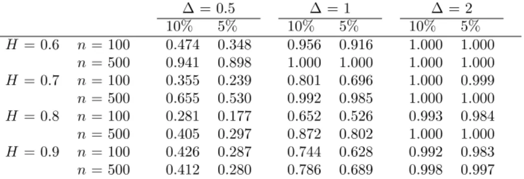
∆ = 0.5 ∆ = 1 ∆ = 2 10% 5% 10% 5% 10% 5% H = 0.6 n= 100 0.474 0.348 0.956 0.916 1.000 1.000 n= 500 0.941 0.898 1.000 1.000 1.000 1.000 H = 0.7 n= 100 0.355 0.239 0.801 0.696 1.000 0.999 n= 500 0.655 0.530 0.992 0.985 1.000 1.000 H = 0.8 n= 100 0.281 0.177 0.652 0.526 0.993 0.984 n= 500 0.405 0.297 0.872 0.802 1.000 1.000 H = 0.9 n= 100 0.426 0.287 0.744 0.628 0.992 0.983 n= 500 0.412 0.280 0.786 0.689 0.998 0.997
Table 3: Empirical power of the self-normalized Wilcoxon change-point test for fractional Gaussian noise of lengthn= 100 andn= 500 with Hurst parameterH and a level shift in the mean of height ∆ after a proportionτ= 0.5. The calculations are based on 5,000 simulation runs.
be rather slow under the hypothesis (see Dehling, Rooch and Taqqu (2013a), Table 2), whereas the size of the self-normalized Wilcoxon change-point test is still close to the corresponding level of significance. We consider fractional Gaussian noise time series with a level shift of height ∆ after a proportion τ of the data in order to analyse the behaviour of the test statistic under the alternative. We have done so for several choices of ∆ andτ and for sample sizesn= 100 and n= 500.
∆ = 0.5 ∆ = 1 ∆ = 2 10% 5% 10% 5% 10% 5% H = 0.6 n= 100 0.321 0.204 0.813 0.690 1.000 1.000 n= 500 0.795 0.678 1.000 0.999 1.000 1.000 H = 0.7 n= 100 0.222 0.125 0.570 0.401 0.989 0.968 n= 500 0.437 0.309 0.948 0.891 1.000 1.000 H = 0.8 n= 100 0.195 0.106 0.417 0.265 0.931 0.839 n= 500 0.264 0.164 0.682 0.530 0.999 0.995 H = 0.9 n= 100 0.339 0.198 0.578 0.403 0.961 0.889 n= 500 0.312 0.186 0.612 0.442 0.989 0.966
Table 4: Empirical power of the self-normalized Wilcoxon change-point test for fractional Gaussian noise of lengthn= 100 andn= 500 with Hurst parameterH and a level shift in the mean of height ∆ after a proportionτ= 0.25. The calculations are based on 5,000 simulation runs.
The simulations of the empirical power confirm that the rejection rate becomes higher when ∆ increases. Comparing the empirical power for different Hurst parameters H, we note that the test tends to have less power asH becomes large. This seems natural since when there is very strong dependence, i.e. H
is large, the variance of the series increases, so that it becomes harder to detect a level shift of a fixed height. In addition, change-points that are located in the middle of the sample are detected more often than change-points that are located close to the boundary of the testing region determined by [τ1, τ2].
Furthermore, Table 4 and Table 3 show that an increasing sample size goes along with an increase of the empirical power. This result confirms that the self-normalized Wilcoxon change-point test yields a consistent discrimination between hypothesis and alternative.
4 Proofs
In order to simplify notation, we write
J(x) = 1
m!Jm(x),
Z(λ) =Zm(λ).
Proof of Theorem 1. The essential step in the proof of Theorem 1 is to find a representation for the test statisticTn(τ1, τ2) as a functional of the Wilcoxon process
Wn(λ) = 1 ndn bnλc X i=1 n X j=bnλc+1 1{Xi≤Xj}− 1 2 , 0≤λ≤1.
For this purpose, rewrite
Gn(k) = k P i=1 n P j=k+1 1{Xi≤Xj}− 1 2 ( 1 n k P t=1 S2 t(1, k) +n1 n P t=k+1 S2 t(k+ 1, n) )12 = 1 ndn k P i=1 n P j=k+1 1{Xi≤Xj}− 1 2 1 ndn ( 1 n k P t=1 S2 t(1, k) +n1 n P t=k+1 S2 t(k+ 1, n) )12 . As we have 1 ndn k X i=1 n X j=k+1 1{Xi≤Xj}− 1 2 =|Wn(λ)|
for the numerator of Gn(k) if k = bnλc, it remains to show that the denominator of Gn(k) can be
represented as a functional of Wn. Since
Ri=n+ 1− n
X
j=1
1{Xi≤Xj}
almost surely, it follows that
St(1, k) =− t X h=1 n X j=1 1{Xh≤Xj}− 1 k k X i=1 n X j=1 1{Xi≤Xj} =− ( t X i=1 n X j=t+1 1{Xi≤Xj}− 1 2 + t X i=1 t X j=1 1{Xi≤Xj}− 1 2 − t k k X i=1 n X j=k+1 1{Xi≤Xj}− 1 2 − t k k X i=1 k X j=1 1{Xi≤Xj}− 1 2 )
almost surely. Moreover, it is well known that
l X i=1 l X j=1 1{Xi≤Xj}= l(l+ 1) 2 . (3) Hence, l X i=1 l X j=1 1{Xi≤Xj}− 1 2 =l(l+ 1) 2 − l2 2 = l 2,
so that St(1, k) =− ( t X i=1 n X j=t+1 1{Xi≤Xj}− 1 2 + t 2− t k k X i=1 n X j=k+1 1{Xi≤Xj}− 1 2 − t k k 2 ) =− ( t X i=1 n X j=t+1 1{Xi≤Xj}− 1 2 − t k k X i=1 n X j=k+1 1{Xi≤Xj}− 1 2 )
almost surely. Thus, if λ∈[τ1, τ2],
Z λ 0 bnrc X i=1 n X j=bnrc+1 1{Xi≤Xj}− 1 2 − bnrc bnλc bnλc X i=1 n X j=bnλc+1 1{Xi≤Xj}− 1 2 2 dr = bnλc X t=0 Z t+1n t n bnrc X i=1 n X j=bnrc+1 1{Xi≤Xj}− 1 2 − bnrc bnλc bnλc X i=1 n X j=bnλc+1 1{Xi≤Xj}− 1 2 2 dr − Z bnλnc+1 λ bnrc X i=1 n X j=bnrc+1 1{Xi≤Xj}− 1 2 −bnrc bnλc bnλc X i=1 n X j=bnλc+1 1{Xi≤Xj}− 1 2 2 dr, where bnrc X i=1 n X j=bnrc+1 1{Xi≤Xj}− 1 2 − bnrc bnλc bnλc X i=1 n X j=bnλc+1 1{Xi≤Xj}− 1 2 = 0
forr∈hλ,bnλnc+1. Therefore, the integral over that interval equals 0. Consequently,
Z λ 0 bnrc X i=1 n X j=bnrc+1 1{Xi≤Xj}− 1 2 − bnrc bnλc bnλc X i=1 n X j=bnλc+1 1{Xi≤Xj}− 1 2 2 dr = bnλc X t=0 Z t+1n t n bnrc X i=1 n X j=bnrc+1 1{Xi≤Xj}− 1 2 − bnrc bnλc bnλc X i=1 n X j=bnλc+1 1{Xi≤Xj}− 1 2 2 dr = 1 n k X t=0 t X i=1 n X j=t+1 1{Xi≤Xj}− 1 2 − t k k X i=1 n X j=k+1 1{Xi≤Xj}− 1 2 2 = 1 n k X t=1 St2(1, k) almost surely in casek=bnλc.
For the second term in the denominator ofGn(k) the following equations hold almost surely
St(k+ 1, n) =− ( t X h=k+1 n X j=1 1{Xh≤Xj}− 1 n−k n X i=k+1 n X j=1 1{Xi≤Xj} ) =− ( t X i=1 n X j=t+1 1{Xi≤Xj}− 1 2 + t X i=1 t X j=1 1{Xi≤Xj}− 1 2 − k X i=1 n X j=k+1 1{Xi≤Xj}− 1 2 − k X i=1 k X j=1 1{Xi≤Xj}− 1 2 − t−k n−k n X i=k+1 k X j=1 1{Xi≤Xj}− 1 2 − t−k n−k n X i=k+1 n X j=k+1 1{Xi≤Xj}− 1 2 ) .
By (3) we get n X i=k+1 n X j=k+1 1{Xi≤Xj}− 1 2 = (n−k)(n−k+ 1) 2 − (n−k)2 2 = n−k 2 . Furthermore, 1{Xi≤Xj}− 1 2 = 1−1{Xj<Xi}− 1 2 =− 1{Xj≤Xi}− 1 2
almost surely ifi6=j. This yields
St(k+ 1, n) =− ( t X i=1 n X j=t+1 1{Xi≤Xj}− 1 2 + t 2 − k X i=1 n X j=k+1 1{Xi≤Xj}− 1 2 −k 2 − t−k n−k n X i=k+1 k X j=1 1{Xi≤Xj}− 1 2 − t−k n−k n−k 2 ) =− ( t X i=1 n X j=t+1 1{Xi≤Xj}− 1 2 − n−t n−k k X i=1 n X j=k+1 1{Xi≤Xj}− 1 2 ) . We obtain forλ∈[τ1, τ2] Z 1 λ bnrc X i=1 n X j=bnrc+1 1{Xi≤Xj}− 1 2 − n− bnrc n− bnλc bnλc X i=1 n X j=bnλc+1 1{Xi≤Xj}− 1 2 2 dr = n−1 X t=bnλc+1 Z t+1n t n bnrc X i=1 n X j=bnrc+1 1{Xi≤Xj}− 1 2 −n− bnrc n− bnλc bnλc X i=1 n X j=bnλc+1 1{Xi≤Xj}− 1 2 2 dr + Z bnλnc+1 λ bnrc X i=1 n X j=bnrc+1 1{Xi≤Xj}− 1 2 − n− bnrc n− bnλc bnλc X i=1 n X j=bnλc+1 1{Xi≤Xj}− 1 2 2 dr
almost surely, where bnrc X i=1 n X j=bnrc+1 1{Xi≤Xj}− 1 2 −n− bnrc n− bnλc bnλc X i=1 n X j=bnλc+1 1{Xi≤Xj}− 1 2 = 0
ifr∈hλ,bnλnc+1. Therefore, the integral over that interval equals 0. Fork=bnλcthis implies
Z 1 λ bnrc X i=1 n X j=bnrc+1 1{Xi≤Xj}− 1 2 −n− bnrc n− bnλc bnλc X i=1 n X j=bnλc+1 1{Xi≤Xj}− 1 2 2 dr = 1 n n−1 X t=k+1 t X i=1 n X j=t+1 1{Xi≤Xj}− 1 2 − n−t n−k k X i=1 n X j=k+1 1{Xi≤Xj}− 1 2 2 = 1 n n−1 X t=k+1 St2(k+ 1, n) = 1 n n X t=k+1 St2(k+ 1, n).
Due to the previous considerations, the properly normalized denominator ofGn(k) can (almost surely)
be represented as follows 1 ndn ( 1 n k X t=1 St2(1, k) + 1 n n X t=k+1 St2(k+ 1, n) )12
= ( Z λ 0 Wn(r)− cn(r) cn(λ) Wn(λ) 2 dr+ Z 1 λ Wn(r)− 1−cn(r) 1−cn(λ) Wn(λ) 2 dr )12 ,
where cn(λ) =bnλnc forλ∈[0,1]. All in all, this yields
Tn(τ1, τ2) = sup λ∈[τ1,τ2] |Wn(λ)| Rλ 0 Wn(r)− cn(r) cn(λ)Wn(λ) 2 dr+R1 λ Wn(r)− 1−cn(r) 1−cn(λ)Wn(λ) 2 dr 12 .
The foregoing characterization of the self-normalized Wilcoxon test statistic points out that a repre-sentation of Tn(τ1, τ2) as a functional of the process
Wn(λ) = 1 ndn bnλc X i=1 n X j=bnλc+1 1{Xi≤Xj}− 1 2 , 0≤λ≤1,
also depends on the function series (cn)n∈Nin D[0,1] defined bycn(λ) = bnλnc, 0≤λ≤1. Since
sup λ∈[0,1] bnλc n −λ = sup λ∈[0,1] λ−bnλc n ≤ sup λ∈[0,1] λ−nλ−1 n = 1 n −→0,
the sequencecn,n∈N, converges with respect to the supremum norm toc∈D[0,1] defined byc(λ) =λ
forλ∈[0,1]. To simplify subsequent calculations, we treat cn andcas random variables with values in
the closure of M = f ∈D[0,1]|f(λ) = bnλc n for some n∈N, n≥ 1 τ1 . Note that hn = cn Wn D −→ c W∗ m , where Wm∗(λ) = (Z(λ)−λZ(1)) Z R J(x)dF(x), 0≤λ≤1. (4)
Obviously, the self-normalized Wilcoxon test statistic can be represented as a functional of the random vector hn. Hence, an application of the continuous mapping theorem just requires the definition of an
appropriate functionG:M×D[0,1]−→Rthat mapshn onTn(τ1, τ2) =G(hn). Forλ∈[τ1, τ2] consider
the function Gλ:M×D[0,1]−→Rthat maps an element h= (h1, h2) on
|h2(λ)| Rλ 0 h2(r)−hh1(r) 1(λ)h2(λ) 2 dr+R1 λ h2(r)−11−−hh1(r) 1(λ)h2(λ) 2 dr 12 ,
provided that the functionF :M×D[0,1]−→Rdefined by
F(h) = inf λ∈[τ1,τ2] ( Z λ 0 h2(r)− h1(r) h1(λ) h2(λ) 2 dr+ Z 1 λ h2(r)− 1−h1(r) 1−h1(λ) h2(λ) 2 dr )12
does not equal 0 inh. Given thath∈F−1({0}), we set Gλ(h) =−1.
Since Tn(τ1, τ2) = supλ∈[τ1,τ2]Gλ(hn), we intend to apply the continuous mapping theorem to the
function G : M ×D[0,1] −→ R, where G(h) = supλ∈[τ1,τ2]Gλ(h). Thus, we have to verify that the
functionGcomplies with the requirements of the continuous mapping theorem, i.e. we have to prove the following assertions:
2) We haveP(h∈DG) = 0, whereDG denotes the set of discontinuities ofG.
In order to show thatGis measurable, we consider the restrictions ofGto M ×D[0,1]
\F−1({0})
and F−1({0}), respectively. Both restrictions are continuous with respect to the uniform metric. In
particular, both restrictions are Borel measurable. Since the restricted domains are Borel measurable subsets ofM×D[0,1], the measurability of the restrictions implies the measurability ofG.
It remains to show that P(h ∈ DG) = 0. Again, consider the restriction of G to M ×D[0,1]
\
F−1({0}). Because of the continuity of the restriction, G is continuous at every h ∈ M×D[0,1]
\
F−1({0}) asF−1({0}) is a closed subset ofM ×D[0,1]. Therefore,D
G is a subset ofF−1({0}).
Conse-quently, it suffices to show thatP(h∈F−1({0})) = 0 in order to prove thatP(h∈D
G) = 0.
The random vector h= (c, Wm∗) is an element ofF−1({0}) if and only if the expression
inf λ∈[τ1,τ2] ( Z λ 0 f(r)− r λf(λ) 2 dr+ Z 1 λ f(r)− 1−r 1−λf(λ) 2 dr )12 (5) vanishes whenf =Wm∗. Note that Wm∗(r)−r λW ∗ m(λ) = Z J(x)dF(x)n(Z(r)−rZ(1))−r λ(Z(λ)−λZ(1)) o = Z J(x)dF(x)nZ(r)− r λZ(λ) o (6) and Wm∗(r)−1−r 1−λW ∗ m(λ) = Z J(x)dF(x) (Z(r)−rZ(1))−1−r 1−λ(Z(λ)−λZ(1)) = Z J(x)dF(x) Z(r)−Z(λ)−r−λ 1−λ(Z(1)−Z(λ)) . (7)
Therefore, and as Z ∈ C[0,1] almost surely (see Maejima and Tudor (2007)), the term in formula (5) vanishes if for someλ∈[τ1, τ2]
( Z λ 0 (Vm(r; 0, λ))2dr+ Z 1 λ (Vm(r;λ,1))2dr )12 = 0, where Vm(r;r1, r2) =Z(r)−Z(r1)− r−r1 r2−r1 (Z(r2)−Z(r1)).
It suffices to show that the sample paths ofWm∗ do not belong to the set of continuous functionsf that satisfy ( Z λ 0 f(r)− r λf(λ) 2 dr+ Z 1 λ f(r)−f(λ)−r−λ 1−λ(f(1)−f(λ)) 2 dr )12 = 0 (8)
for some λ ∈ [τ1, τ2]. The above equation only holds if the integrands vanish almost surely on the
corresponding intervals. In particular, a continuous function f ∈D[0,1] that meets formula (8) satisfies
f(r) = 1 λf(λ)r ifr∈[0, λ] and f(r) =f(λ) +r−λ 1−λ{f(1)−f(λ)} =f(λ)− λ 1−λ{f(1)−f(λ)}+ 1 1−λ{f(1)−f(λ)}r
ifr∈[λ,1]. Consequently, the set of continuous functions which lie inF−1({0}) corresponds to the class
of functions
A=nf ∈D[0,1]| for someλ∈[τ1, τ2] and a, b∈R
f(r) = 1 λar on [0, λ] and f(r) =a− λ 1−λ{b−a}+ 1 1−λ{b−a}ron [λ,1] o .
It follows thatP(Z∈A) = 0 because the sample paths of the Hermite processZare nowhere differentiable with probability 1 (see Mikosch (1998)), whereas an element in A is differentiable almost everywhere. This impliesP(h∈DG) = 0.
Having verified the preconditions of the continuous mapping theorem we are now able to conclude that the test statisticTn(τ1, τ2) converges in distribution to
T(m, τ1, τ2) = sup λ∈[τ1,τ2] |Wm∗(λ)| Rλ 0 Wm∗(r)−rλWm∗(λ) 2 dr+Rλ1W∗ m(r)−11−−λrWm∗(λ) 2 dr 12 .
Due to (6) and (7), the limit processT(m, τ1, τ2) equals
sup λ∈[τ1,τ2] |Z(λ)−λZ(1)| nRλ 0 (Vm(r; 0, λ)) 2 dr+Rλ1(Vm(r;λ,1)) 2 dro 1 2 .
Thus, we have established Theorem 1.
In the proof of Theorem 2 we make use of preliminary results stated in Lemma 1, Lemma 2 and Corollary 1. The line of argument that verifies Lemma 1 and Lemma 2 is a modification of the proof that establishes Theorem 3.1 in Dehling, Rooch and Taqqu (2013b).
Lemma 1. Suppose that (ξi)i≥1 is a stationary, long-range dependent Gaussian process with mean 0,
variance 1 and LRD parameter0< D < 1
m, wheremdenotes the Hermite rank of the class of functions
1{G(ξi)≤x}−F(x), x∈ R. Moreover, assume that (G(ξi))i≥1 has a continuous distribution function F
and that G:R−→Ris a measurable function. Then, if ∆∈R,
1 n2 bnλc X i=1 n X j=bnτc+1 1{G(ξi)≤G(ξj)+∆} P −→λ(1−τ) Z R F(x+ ∆)dF(x), 1 n2 bnτc X i=1 n X j=bnλc+1 1{G(ξi)≤G(ξj)+∆} P −→τ(1−λ) Z R F(x+ ∆)dF(x)
for fixed τ, uniformly inλ≤τ andλ≥τ, respectively.
Proof of Lemma 1. We give a proof for the first assertion only as the convergence of the second term follows by an analogous argumentation.
LetFk andFk+1,ndenote the empirical distribution functions of the firstkand lastn−krealizations
ofG(ξ1), . . . , G(ξn), i.e. Fk(x) = 1 k k X i=1 1{G(ξi)≤x}, Fk+1,n(x) = 1 n−k n X i=k+1 1{G(ξi)≤x}. Forλ≤τ this yields the following representation:
bnλc X i=1 n X j=bnτc+1 1{G(ξi)≤G(ξj)+∆}= (n− bnτc)bnλc 1 n− bnτc n X j=bnτc+1 Fbnλc(G(ξj) + ∆)
= (n− bnτc)bnλc
Z
R
Fbnλc(x+ ∆)dFbnτc+1,n(x)
Since n−bnnτc −→ 1 −τ, it suffices to show that bnλcR
RFbnλc(x+ ∆)dFbnτc+1,n(x) converges to
λR
RF(x+ ∆)dF(x). For this purpose, we consider the inequality
sup 0≤λ≤τ 1 nbnλc Z R Fbnλc(x+ ∆)dFbnτc+1,n(x)−λ Z R F(x+ ∆)dF(x) (9) ≤ sup 0≤λ≤τ 1 n Z R bnλcFbnλc(x+ ∆)dFbnτc+1,n(x)− bnλc n Z R F(x+ ∆)dFbnτc+1,n(x) + sup 0≤λ≤τ bnλc n Z R F(x+ ∆)dFbnτc+1,n(x)−λ Z R F(x+ ∆)dFbnτc+1,n(x) + sup 0≤λ≤τ λ Z R F(x+ ∆)dFbnτc+1,n(x)−λ Z R F(x+ ∆)dF(x)
and we will show that each of the three terms on its right-hand side converges to 0. For the third summand we get
sup 0≤λ≤τ λ Z R F(x+ ∆)dFbnτc+1,n(x)−λ Z R F(x+ ∆)dF(x) = sup 0≤λ≤τ λ 1− Z R Fbnτc+1,n(x)dF(x+ ∆)− 1− Z R F(x)dF(x+ ∆) =τ Z R Fbnτc+1,n(x)−F(x) dF(x+ ∆) ≤τsup x∈R Fbnτc+1,n(x)−F(x)
as a consequence of integration by parts. Furthermore, we have sup
x∈R
|Fn(x)−F(x)| −→0 a.s.
by an application of the Glivenko-Cantelli theorem (see Krengel and Brunel (1985)) to the stationary and ergodic process (G(ξi))i≥1. So as to deduce an analogous result forFbnτc+1,n we rewrite
Fbnτc+1,n(x) =
n
n− bnτcFn(x)− bnτc
n− bnτcFbnτc(x)
and we may therefore conclude
Fbnτc+1,n(x)−F(x) ≤ n n− bnτc |Fn(x)−F(x)|+ bnτc n− bnτc Fbnτc(x)−F(x) . Thus, sup x∈R Fbnτc+1,n(x)−F(x) −→0 a.s. (10)
which implies that the third term on the right-hand side of (9) converges to 0 almost surely. Regarding the second term on the right-hand side of (9), we obtain
sup 0≤λ≤τ bnλc n Z R F(x+ ∆)dFbnτc+1,n(x)−λ Z R F(x+ ∆)dFbnτc+1,n(x) = sup 0≤λ≤τ bnλc n −λ Z R F(x+ ∆)dFbnτc+1,n(x) .
The right-hand side of this equation converges to 0 since R RF(x+ ∆)dFbnτc+1,n(x) is bounded by 1, and as sup 0≤λ≤τ bnλc n −λ −→0.
In order to show that the first term in (9) converges to 0 as well, we consider the following inequality: sup 0≤λ≤τ 1 n Z R bnλcFbnλc(x+ ∆)dFbnτc+1,n(x)− bnλc n Z R F(x+ ∆)dFbnτc+1,n(x) (11) = sup 0≤λ≤τ 1 n Z R bnλc Fbnλc(x+ ∆)−F(x+ ∆) dFbnτc+1,n(x) ≤ sup 0≤λ≤τ dn n Z R d−n1bnλc Fbnλc(x+ ∆)−F(x+ ∆)−J(x+ ∆)Z(λ)dFbnτc+1,n(x) + sup 0≤λ≤τ dn nZ(λ) Z R J(x+ ∆)dFbnτc+1,n(x)
In what follows, we will prove that both terms on the right-hand side of (11) converge to 0. For this purpose, we make use of the empirical process non-central limit theorem of Dehling and Taqqu (1989) which states that
d−n1bnλc(Fbnλc(x)−F(x))x∈[−∞,∞],λ∈[0,1] D
−→J(x)Z(λ),
where “−→D ” denotes convergence in distribution with respect to theσ-field generated by the open balls in D([−∞,∞]×[0,1]), equipped with the supremum norm.
Due to the Dudley-Wichura version of Skorohod’s representation theorem (see Shorack and Wellner (1986), Theorem 2.3.4), we may assume without loss of generality that
sup λ,x d−n1bnλc Fbnλc(x)−F(x) −J(x)Z(λ)−→0
almost surely; see Dehling, Rooch and Taqqu (2013a). As a consequence, the first summand in (11) converges to 0 since sup 0≤λ≤τ dn n Z R d−n1bnλc Fbnλc(x+ ∆)−F(x+ ∆) −J(x+ ∆)Z(λ)dFbnτc+1,n(x) = dn n 0≤supλ≤τ,x d−n1bnλc Fbnλc(x+ ∆)−F(x+ ∆)−J(x+ ∆)Z(λ) and as dn n converges to 0 as well.
For the second summand we get the following inequality: sup 0≤λ≤τ dn nZ(λ) Z R J(x+ ∆)dFbnτc+1,n(x) ≤ dn n 0≤supλ≤τ |Z(λ)| Z R J(x+ ∆)dFbnτc+1,n(x) Note that J(x) = Z R 1{G(y)≤x}Hm(y)ϕ(y)dy = Z R Hm(y)ϕ(y)dy− Z R 1{x≤G(y)}Hm(y)ϕ(y)dy =− Z R 1{x≤G(y)}Hm(y)ϕ(y)dy,
where ϕdenotes the standard normal density function, since
Z
R
Hm(y)ϕ(y)dy= 0.
For this reason, we have
Z R J(x+ ∆)dFbnτc+1,n(x) =− Z R Z R 1{x+∆≤G(y)}Hm(y)ϕ(y)dydFbnτc+1,n(x) =− Z R Z R 1{x+∆≤G(y)}dFbnτc+1,n(x)Hm(y)ϕ(y)dy
=− Z R Fbnτc+1,n(G(y)−∆)Hm(y)ϕ(y)dy and Z R J(x+ ∆)dF(x) =− Z R Z R 1{x+∆≤G(y)}Hm(y)ϕ(y)dydF(x) =− Z R Z R 1{x+∆≤G(y)}dF(x)Hm(y)ϕ(y)dy =− Z R F(G(y)−∆)Hm(y)ϕ(y)dy.
Regarding the difference of these terms, we obtain
Z R J(x+ ∆)dFbnτc+1,n(x)− Z R J(x+ ∆)dF(x) = Z R F(G(y)−∆)−Fbnτc+1,n(G(y)−∆) Hm(y)ϕ(y)dy ≤ Z R F(G(y)−∆)−Fbnτc+1,n(G(y)−∆) |Hm(y)|ϕ(y)dy ≤sup y∈R F(G(y)−∆)−Fbnτc+1,n(G(y)−∆) Z R |Hm(y)|ϕ(y)dy, where R
R|Hm(y)|ϕ(y)dy <∞because of H¨older’s inequality and where
sup y∈R F(G(y)−∆)−Fbnτc+1,n(G(y)−∆) −→0a.s. by (10). As a result, R RJ(x+ ∆)dFbnτc+1,n(x) D −→ R
RJ(x+ ∆)dF(x), so that in the end the second
summand in (11) converges to 0 almost surely, too.
All in all, the third term on the right-hand side of (9) converges to 0 almost surely as it is dominated by the sum of two expressions which both converge to 0 with probability 1. This completes the proof of
the first assertion in Lemma 1.
Corollary 1. Suppose that(ξi)i≥1 is a stationary, long-range dependent Gaussian process with mean0,
variance 1 and LRD parameter0< D < m1, wheremdenotes the Hermite rank of the class of functions
1{G(ξi)≤x}−F(x), x∈ R. Moreover, assume that (G(ξi))i≥1 has a continuous distribution function F
and that G:R−→Ris a measurable function. Then
1 n2 bnτc X i=1 n X j=bnτc+1 1{G(ξi)≤G(ξj)+∆} P −→τ(1−τ) Z R F(x+ ∆)dF(x) for fixed τ.
Proof of Corollary 1. Consider the function G: D[0, τ]−→ R, f 7→f(τ). As G is continuous with
respect to the supremum norm onD[0, τ], Corollary 1 follows from Lemma 1 and the continuous mapping
theorem
Lemma 2. Suppose that (ξi)i≥1 is a stationary, long-range dependent Gaussian process with mean 0,
variance 1 and LRD parameter0< D < 1
m, wheremdenotes the Hermite rank of the class of functions
1{G(ξi)≤x}−F(x), x∈ R. Moreover, assume that (G(ξi))i≥1 has a continuous distribution function F
and that G:R−→Ris a measurable function. Then
1 n2 bnτc X i=1 bnλc X j=bnτc+1 1{G(ξi)≤G(ξj)+∆} P −→τ(λ−τ) Z R F(x+ ∆)dF(x)
Proof of Lemma 2. LetFk+1,t denote the empirical distribution function ofG(ξk+1), . . . , G(ξt), i.e. Fk+1,t(x) = 1 t−k t X i=k+1 1{G(ξi)≤x}. We may therefore rewrite
bnτc X i=1 bnλc X j=bnτc+1 1{G(ξi)≤G(ξj)+∆}= (bnλc − bnτc)bnτc 1 (bnλc − bnτc) bnλc X j=bnτc+1 Fbnτc(G(ξj) + ∆) = (bnλc − bnτc)bnτc Z R Fbnτc(x+ ∆)dFbnτc+1,bnλc(x). Furthermore, repeated application of the triangle inequality yields
sup τ≤λ≤1 1 n(bnλc − bnτc) Z R Fbnτc(x+ ∆)dFbnτc+1,bnλc(x)−(λ−τ) Z R F(x+ ∆)dF(x) (12) ≤ sup τ≤λ≤1 1 n(bnλc − bnτc) Z R Fbnτc(x+ ∆)−F(x+ ∆) dFbnτc+1,bnλc(x) + sup τ≤λ≤1 1 n(bnλc − bnτc) Z R F(x+ ∆)dFbnτc+1,bnλc(x)− 1 n(bnλc − bnτc) Z R F(x+ ∆)dF(x) + sup τ≤λ≤1 1 n(bnλc − bnτc) Z R F(x+ ∆)dF(x)−(λ−τ) Z R F(x+ ∆)dF(x) .
In order to prove that the stochastic process considered in Lemma 2 converges to the given limit process, it is sufficient to show that the expressions on the right-hand side of the above inequality converge to 0. We consider each of the three summands separately.
Apparently, the third term converges to 0 since sup τ≤λ≤1 1 n(bnλc − bnτc) Z R F(x+ ∆)dF(x)−(λ−τ) Z R F(x+ ∆)dF(x) = sup τ≤λ≤1 1 n(bnλc − bnτc)−(λ−τ) Z R F(x+ ∆)dF(x) and as supτ≤λ≤11n(bnλc − bnτc)−(λ−τ) −→0. We have sup τ≤λ≤1 1 n(bnλc − bnτc) Z R Fbnτc(x+ ∆)−F(x+ ∆)dFbnτc+1,bnλc(x) ≤sup x∈R Fbnτc(x+ ∆)−F(x+ ∆) sup τ≤λ≤1 1 n(bnλc − bnτc)
for the first summand. As supx∈RFbnτc(x+ ∆)−F(x+ ∆)
converges to 0 almost surely by the
Glivenko-Cantelli theorem, so does the right-hand side of the above inequality. Finally, consider the second term on the right-hand side of (12). We have
sup τ≤λ≤1 1 n(bnλc − bnτc) Z R F(x+ ∆)dFbnτc+1,bnλc(x)− 1 n(bnλc − bnτc) Z R F(x+ ∆)dF(x) = sup τ≤λ≤1 1 n(bnλc − bnτc) Z R F(x+ ∆)d Fbnτc+1,bnλc−F(x) = sup τ≤λ≤1 1 n(bnλc − bnτc) Z R Fbnτc+1,bnλc(x)−F(x) dF(x+ ∆) =dn n τ≤supλ≤1 Z R d−n1(bnλc − bnτc) Fbnτc+1,bnλc(x)−F(x) −J(x) (Z(λ)−Z(τ))dF(x+ ∆) + sup τ≤λ≤1 dn n (Z(λ)−Z(τ)) Z R J(x)dF(x+ ∆)
≤dn n τ≤λsup≤1,x∈R d−n1(bnλc − bnτc) Fbnτc+1,bnλc(x)−F(x) −J(x) (Z(λ)−Z(τ)) +dn n τ≤supλ≤1 |Z(λ)−Z(τ)| Z R J(x)dF(x+ ∆) .
It follows from integration by parts that
Z R F(x+ ∆)dFbnτc+1,bnλc(x)− Z R F(x+ ∆)dF(x) = Z R F(x)dF(x+ ∆)− Z R Fbnτc+1,bnλc(x)dF(x+ ∆). Furthermore, (bnλc − bnτc) Fbnτc+1,bnλc(x)−F(x)= bnλc X i=bnτc+1 1{G(ξi)≤x}−(bnλc − bnτc)F(x) =bnλcFbnλc(x)− bnτcFbnτc(x)− bnλcF(x) +bnτcF(x) =bnλc Fbnλc(x)−F(x)− bnτc Fbnτc(x)−F(x). As a result, sup τ≤λ≤1,x∈R d−n1(bnλc − bnτc) Fbnτc+1,bnλc(x)−F(x) −J(x) (Z(λ)−Z(τ)) = sup τ≤λ≤1,x∈R d−n1 bnλc Fbnλc(x)−F(x) − bnτc Fbnτc(x)−F(x) −J(x) (Z(λ)−Z(τ)) ≤ sup τ≤λ≤1,x∈R d− 1 n bnλc Fbnλc(x)−F(x) −J(x)Z(λ) + sup τ≤λ≤1,x∈R d−n1bnτc Fbnτc(x)−F(x) −J(x)Z(τ).
Again, we may assume without loss of generality that sup λ,x d−n1bnλc Fbnλc(x)−F(x)−J(x)Z(λ) −→0
almost surely, as pointed out in the proof of Lemma 1. Since dn
n −→ 0 by definition of dn, we may
conclude that the third summand on the right hand side of (12) converges to 0, too. This completes the
proof of Lemma 2.
Proof of Theorem 2. We have
Tn(τ1, τ2) = sup k∈[bnτ1c,bnτ2c] Gn(k) ≥Gn(k∗), where Gn(k∗) = k∗ P i=1 n P j=k∗+1 1{Xi≤Xj}− 1 2 ( 1 n k∗ P t=1 S2 t(1, k∗) +n1 n P t=k∗+1 S2 t(k∗+ 1, n) )12
and wherek∗=bnτcdenotes the location of the change-point. Thus, it suffices to show thatGn(k∗) P −→ ∞. For this purpose, we rewrite
Gn(k∗) = 1 n2 k∗ P i=1 n P j=k∗+1 1{Xi≤Xj}− 1 2 1 n2 ( 1 n k∗ P t=1 S2 t(1, k∗) +n1 n P t=k∗+1 S2 t(k∗+ 1, n) )12 .
We will prove that the numerator ofGn(k∗) converges to a positive constant, whereas the denominator
tends to 0 in order to show divergence to∞. First, we turn to the denominator, which equals
1 n2 Z τ 0 Sb2nrc(1, k∗)dr+ Z 1 τ S2bnrc(k∗+ 1, n)dr 12 .
Note that for i≤k∗
n X j=1 1{Xi≤Xj}= k∗ X j=1 1{µ+G(ξi)≤µ+G(ξj)}+ n X j=k∗+1 1{µ+G(ξi)≤µ+G(ξj)+∆} = n X j=1 1{G(ξi)≤G(ξj)}+ n X j=k∗+1 1{G(ξj)<G(ξi)≤G(ξj)+∆}. Therefore, St(1, k∗) =− t X h=1 n X j=1 1{Xh≤Xj}− 1 k∗ k∗ X i=1 n X j=1 1{Xi≤Xj} =− t X h=1 n X j=1 1{G(ξh)≤G(ξj)}− 1 k∗ k∗ X i=1 n X j=1 1{G(ξi)≤G(ξj)} − t X h=1 n X j=k∗+1 1{G(ξj)<G(ξh)≤G(ξj)+∆}− 1 k∗ k∗ X i=1 n X j=k∗+1 1{G(ξj)<G(ξi)≤G(ξj)+∆} .
We treat the expressionSt(1, k∗) as sum of the following terms
ˆ St(1, k∗) =− t X h=1 n X j=1 1{G(ξh)≤G(ξj)}− 1 k∗ k∗ X i=1 n X j=1 1{G(ξi)≤G(ξj)} , ˜ St(1, k∗) =− t X h=1 n X j=k∗+1 1{G(ξj)<G(ξh)≤G(ξj)+∆}− 1 k∗ k∗ X i=1 n X j=k∗+1 1{G(ξj)<G(ξi)≤G(ξj)+∆} .
For the first summand we get
ˆ St(1, k∗) =− t X h=1 n X j=1 1{G(ξh)≤G(ξj)}− 1 k∗ k∗ X i=1 n X j=1 1{G(ξi)≤G(ξj)} =− t X i=1 t X j=1 1{G(ξi)≤G(ξj)}− t X i=1 n X j=t+1 1{G(ξi)≤G(ξj)} + t k∗ k∗ X i=1 k∗ X j=1 1{G(ξi)≤G(ξj)}+ t k∗ k∗ X i=1 n X j=k∗+1 1{G(ξi)≤G(ξj)} =−t(t+ 1) 2 − t X i=1 n X j=t+1 1{G(ξi)≤G(ξj)}+ t k∗ k∗(k∗+ 1) 2 + t k∗ k∗ X i=1 n X j=k∗+1 1{G(ξi)≤G(ξj)} =−t 2 2 − t X i=1 n X j=t+1 1{G(ξi)≤G(ξj)}+ tk∗ 2 + t k∗ k∗ X i=1 n X j=k∗+1 1{G(ξi)≤G(ξj)}. We have 1 n2 bnλc X i=1 n X j=bnλc+1 1{G(ξi)≤G(ξj)} P −→ λ(1−λ) 2
uniformly inλbecause 1 ndn bnλc X i=1 n X j=bnλc+1 1{G(ξi)≤G(ξj)}− 1 2 D −→(Z(λ)−λZ(1)) Z R J(x)dF(x)
uniformly inλby Theorem 1.1 in Dehling, Rooch and Taqqu (2013a) and as dn
n −→0. We may conclude
from this and Corollary 1 that n12Sˆbnλc(1,bk∗c)
P
−→0 uniformly inλ≤τ. Because of
1{G(ξj)<G(ξi)≤G(ξj)+∆}= 1{G(ξi)≤G(ξj)+∆}−1{G(ξi)≤G(ξj)}, the second summand can be written as
˜ St(1, k∗) =− t X h=1 n X j=k∗+1 1{G(ξj)<G(ξh)≤G(ξj)+∆}− 1 k∗ k∗ X i=1 n X j=k∗+1 1{G(ξj)<G(ξi)≤G(ξj)+∆} =− t X i=1 n X j=k∗+1 1{G(ξi)≤G(ξj)+∆}+ t k∗ k∗ X i=1 n X j=k∗+1 1{G(ξi)≤G(ξj)+∆} + t X i=1 n X j=k∗+1 1{G(ξi)≤G(ξj)}− t k∗ k∗ X i=1 n X j=k∗+1 1{G(ξi)≤G(ξj)}.
Due to Lemma 1 and Corollary 1, n12S˜bnλc(1, k∗) converges in probability to 0, as well. All in all, the previous considerations yield
Z τ 0 1 n2Sbnrc(1, k ∗) 2 dr−→P 0 as G:D[0, τ]−→R,f 7→Rτ 0 (f(s)) 2
ds, is continuous with respect to the supremum norm onD[0, τ]. In analogy to the previous argumentation it can be shown that
Z 1 τ 1 n2Sbnrc(k ∗+ 1, n) 2 dr−→P 0.
For this purpose, note that, ifi > k∗,
n X j=1 1{Xi≤Xj}= k∗ X j=1 1{µ+G(ξi)+∆≤µ+G(ξj)}+ n X j=k∗+1 1{µ+G(ξi)+∆≤µ+G(ξj)+∆} = n X j=1 1{G(ξi)≤G(ξj)}− k∗ X j=1 1{G(ξi)≤G(ξj)<G(ξi)+∆}. Therefore, St(k∗+ 1, n) =− t X h=k∗+1 n X j=1 1{Xh≤Xj}− 1 n−k∗ n X i=k∗+1 n X j=1 1{Xi≤Xj} =− t X h=k∗+1 n X j=1 1{G(ξh)≤G(ξj)}− 1 n−k∗ n X i=k∗+1 n X j=1 1{G(ξi)≤G(ξj)} + t X h=k∗+1 k∗ X j=1 1{G(ξh)≤G(ξj)<G(ξh)+∆}− 1 n−k∗ n X i=k∗+1 k∗ X j=1 1{G(ξi)≤G(ξj)<G(ξi)+∆} .
Hence, we considerSt(k∗+ 1, n) as sum of the expressions below
ˆ St(k∗+ 1, n) =− t X h=k∗+1 n X j=1 1{G(ξh)≤G(ξj)}− 1 n−k∗ n X i=k∗+1 n X j=1 1{G(ξi)≤G(ξj)} ,
˜ St(k∗+ 1, n) = t X h=k∗+1 k∗ X j=1 1{G(ξh)≤G(ξj)<G(ξh)+∆}− 1 n−k∗ n X i=k∗+1 k∗ X j=1 1{G(ξi)≤G(ξj)<G(ξi)+∆} .
The following representation arises from rather simple transformations
ˆ St(k∗+ 1, n) =− t X h=k∗+1 n X j=1 1{G(ξh)≤G(ξj)}− 1 n−k∗ n X i=k∗+1 n X j=1 1{G(ξi)≤G(ξj)} =− t X i=1 n X j=t+1 1{G(ξi)≤G(ξj)}− t X i=1 t X j=1 1{G(ξi)≤G(ξj)} + k∗ X i=1 n X j=k∗+1 1{G(ξi)≤G(ξj)}+ k∗ X i=1 k∗ X j=1 1{G(ξi)≤G(ξj)} + t−k ∗ n−k∗ n X i=k∗+1 k∗ X j=1 1{G(ξi)≤G(ξj)}+ t−k∗ n−k∗ n X i=k∗+1 n X j=k∗+1 1{G(ξi)≤G(ξj)} =− t X i=1 n X j=t+1 1{G(ξi)≤G(ξj)}− t(t+ 1) 2 + k∗ X i=1 n X j=k∗+1 1{G(ξi)≤G(ξj)}+ k∗(k∗+ 1) 2 + t−k ∗ n−k∗ n X i=k∗+1 k∗ X j=1 1−1{G(ξj)≤G(ξi)} + t−k ∗ n−k∗ (n−k∗)(n−k∗+ 1) 2 =− t X i=1 n X j=t+1 1{G(ξi)≤G(ξj)}− t(t+ 1) 2 + k∗ X i=1 n X j=k∗+1 1{G(ξi)≤G(ξj)}+ k∗(k∗+ 1) 2 + (t−k∗)k∗− t−k ∗ n−k∗ k∗ X j=1 n X i=k∗+1 1{G(ξj)≤G(ξi)}+ (t−k∗)(n−k∗+ 1) 2 .
Based on Lemma 1 and Corollary 1, the argumentation that also established n12Sˆbnλc(1, k∗)
P −→0 yields 1 n2Sˆbnλc(k∗+ 1, n) P −→0 uniformly inλ≥τ. Likewise, it can be shown that n12S˜bnλc(k∗+ 1, n)
P
−→0. First of all, we note that 1{G(ξi)≤G(ξj)<G(ξi)+∆}= 1{G(ξj)≤G(ξi)+∆}−1{G(ξj)≤G(ξi)} almost surely ifi6=j. Thereby,
˜ St(k∗+ 1, n) = t X h=k∗+1 k∗ X j=1 1{G(ξh)≤G(ξj)<G(ξh)+∆}− 1 n−k∗ n X i=k∗+1 k∗ X j=1 1{G(ξi)≤G(ξj)<G(ξi)+∆} = k∗ X j=1 t X i=k∗+1 1{G(ξj)≤G(ξi)+∆}− t−k∗ n−k∗ k∗ X j=1 n X i=k∗+1 1{G(ξj)≤G(ξi)+∆} − k∗ X j=1 t X i=k∗+1 1{G(ξj)≤G(ξi)}+ t−k∗ n−k∗ k∗ X j=1 n X i=k∗+1 1{G(ξj)≤G(ξi)}. As a result, we have 1 n2S˜bnλc(k∗+ 1, n) P
−→0 by Lemma 2 and Corollary 1. As both terms, 1
n2Sˆbnλc(k∗+ 1, n) as well as n12S˜bnλc(k∗+ 1, n), converge in probability to 0 uniformly in λ≥τ, it follows that Z 1 τ 1 n2Sbnrc(k ∗+ 1, n) 2 dr−→P 0.
On the basis of the previous considerations we may conclude that the denominator ofGn(k∗) converges
In order to prove the consistency of the self-normalized Wilcoxon change-point test, it therefore remains to show that the numerator ofGn(k∗), given by
1 n2 k∗ X i=1 n X j=k∗+1 1{Xi≤Xj}− 1 2 ,
converges to a non-negative constant. We have 1 n2 k∗ X i=1 n X j=k∗+1 1{Xi≤Xj}− 1 2 = 1 n2 k∗ X i=1 n X j=k∗+1 1{G(ξi)≤G(ξj)+∆}− 1 n2 k∗(n−k∗) 2 . Therefore, 1 n2 k∗ X i=1 n X j=k∗+1 1{Xi≤Xj}− 1 2 P −→τ(1−τ) Z R (F(x+ ∆)−F(x))dF(x) (13)
by Corollary 1 and since n12
k∗(n−k∗) 2 −→
τ(1−τ)
2 . As the limit in (13) does not vanish, Gn(k
∗) diverges
to ∞and we thus have proved Theorem 2.
Proof of Theorem 3. Note that because of the corresponding sample path properties of the stochastic processZ, the sample paths of
Wm,τ∗ (λ) = (Z(λ)−λZ(1)) Z R J(x)dF(x) +cδτ(λ) Z R f2(x)dx, 0≤λ≤1,
are almost surely continuous and nowhere differentiable.
The same argument as in the proof of Theorem 1 shows thatTn(τ1, τ2) converges in distribution to
sup λ∈[τ1,τ2] Wm,τ∗ (λ) Rλ 0 W ∗ m,τ(r)− r λW ∗ m,τ(λ) 2 dr+R1 λ W∗ m,τ(r)− 1−r 1−λW ∗ m,τ(λ) 2 dr 12 .
The numerator of the limit process equals
Z R J(x)dF(x) (Z(λ)−λZ(1)) +cδτ(λ) Z R f2(x)dx .
Moreover, for the quantities in the denominator it holds that
Wm,τ∗ (r)− r λW ∗ m,τ(λ) = (Z(r)−rZ(1)) Z R J(x)dF(x) +cδτ(r) Z R f2(x)dx −r λ (Z(λ)−λZ(1)) Z R J(x)dF(x) +cδτ(λ) Z R f2(x)dx = Z R J(x)dF(x)Z(λ)− r λZ(λ) +c Z R f2(x)dxδτ(r)− r λδτ(λ) and Wm,τ∗ (r)− 1−r 1−λW ∗ m,τ(λ) = (Z(r)−rZ(1)) Z R J(x)dF(x) +cδτ(r) Z R f2(x)dx − 1−r 1−λ (Z(λ)−λZ(1)) Z R J(x)dF(x) +cδτ(λ) Z R f2(x)dx = Z R J(x)dF(x) Z(r)−rZ(1)− 1−r 1−λ(Z(λ)−λZ(1)) +c Z R f2(x)dx δτ(r)− 1−r 1−λδτ(λ) .
References
Andrews, D. W. K. (1993) Tests for Parameter Instability and Structural Change with Unknown Change Point.Econometrica 61, 821–856.
Dehling, H. G., Rooch, A., and Taqqu, M. S. (2013a) Non-Parametric Change-Point Tests for Long-Range Dependent Data.Scandinavian Journal of Statistics 40, 153 – 173.
Dehling, H. G., Rooch, A., and Taqqu, M. S. (2013b) Power of Change-Point Tests for Long-Range Dependent Data. arXiv:1303.4917.
Dehling, H. G. and Taqqu, M. S. (1989) The Empirical Process of some Long-Range Dependent Sequences with an Application to U-Statistics. The Annals of Statistics17, 1767–1783.
Krengel, U. and Brunel, A. (1985)Ergodic theorems. Walter de Gruyter Berlin, New York.
Lobato, I. N. (2001) Testing That a Dependent Process Is Uncorrelated.Journal of the American Statis-tical Association 96, 1066–1076.
Maejima, M. and Tudor, C. A. (2007) Wiener integrals with respect to the Hermite process and a Non-Central Limit Theorem.Stochastic Analysis and Applications 25, 1043–1056.
Mikosch, T. (1998) Elementary Stochastic Calculus With Finance in View. World Scientific Publishing Co. Pte. Ltd.
Shao, X. (2011) A simple test of changes in mean in the possible presence of long-range dependence.
Journal of Time Series Analysis 32(6), 598–606.
Shao, X. and Zhang, X. (2010) Testing for Change Points in Time Series. Journal of The American Statistical Association 105, 1228–1240.
Shorack, G. R. and Wellner, J. A. (1986)Empirical Processes with Applications to Statistics. John Wiley & Sons, New York.
Taqqu, M. S. (1979) Convergence of Integrated Processes of Arbitrary Hermite Rank. Zeitschrift f¨ur Wahrscheinlichkeitstheorie und verwandte Gebiete 50, 53–83.
![Table 1: Simulated critical values for the distribution of T (1, τ 1 , τ 2 ) when [τ 1 , τ 2 ] = [0.15, 0.85]](https://thumb-us.123doks.com/thumbv2/123dok_us/9459803.2820496/8.892.154.741.136.262/table-simulated-critical-values-distribution-t-τ-τ.webp)