Boise State University
ScholarWorks
Mathematics Faculty Publications and Presentations
Department of Mathematics
2-15-2017
Stable Computations with Flat Radial Basis
Functions Using Vector-Valued Rational
Approximations
Grady B. Wright
Boise State UniversityBengt Fornberg
University of ColoradoThis is an author-produced, peer-reviewed version of this article. © 2017, Elsevier. Licensed under the Creative Commons
Attribution-Publication Information
Wright, Grady B. and Fornberg, Bengt. (2017). "Stable Computations with Flat Radial Basis Functions Using Vector-Valued Rational Approximations".Journal of Computational Physics, 331, 137-156.http://dx.doi.org/10.1016/j.jcp.2016.11.030
Stable computations with flat radial basis functions using vector-valued
rational approximations
Grady B. Wrighta,∗, Bengt Fornbergb
aDepartment of Mathematics, Boise State University, Boise, ID 83725-1555, USA bDepartment of Applied Mathematics, University of Colorado, 526 UCB, Boulder, CO 80309, USA
Abstract
One commonly finds in applications of smooth radial basis functions (RBFs) that scaling the kernels so they are ‘flat’ leads to smaller discretization errors. However, the direct numerical approach for computing with flat RBFs (RBF-Direct) is severely ill-conditioned. We present an algorithm for bypassing this ill-conditioning that is based on a new method for rational approximation (RA) of vector-valued analytic functions with the property that all components of the vector share the same singularities. This new algorithm (RBF-RA) is more accurate, robust, and easier to implement than the Contour-Pad´e method, which is similarly based on vector-valued rational approximation. In contrast to the stable RBF-QR and RBF-GA algorithms, which are based on finding a better conditioned base in the same RBF-space, the new algorithm can be used with any type of smooth radial kernel, and it is also applicable to a wider range of tasks (including calculating Hermite type implicit RBF-FD stencils). We present a series of numerical experiments demonstrating the effectiveness of this new method for computing RBF interpolants in the flat regime. We also demonstrate the flexibility of the method by using it to compute implicit RBF-FD formulas in the flat regime and then using these for solving Poisson’s equation in a 3-D spherical shell.
Keywords: RBF, shape parameter, ill-conditioning, Contour-Pad´e, RBF-QR, RBF-GA, rational approximation, common denominator, RBF-FD, RBF-HFD
1. Introduction
Meshfree methods based on smooth radial basis functions (RBFs) are finding increasing use in scientific computing as they combine high order accuracy with enormous geometric flexibility in applications such as interpolation and for numerically solving PDEs. In these applications, one finds that the best accuracy is often achieved when their shape parameterεis small, meaning that they are relatively flat [1, 2].
The so called Uncertainty Principle, formulated in 1995 [3], has contributed to a widespread misconception that flat radial kernels unavoidably lead to numerical ill-conditioning. This ‘principle’ mistakenly assumes that RBF interpolants need to be computed by solving the standard RBF linear system (often denoted RBF-Direct). However, it has now been known for over a decade [4–7] that the ill-conditioning issue is specific to this RBF-Direct approach, and that it can be avoided using alternative methods. Three distinctly different numerical algorithms have been presented thus far in the literature for avoiding this ill-conditioning
and thus open up the complete range ofεthat can be considered. These are the Contour-Pad´e (RBF-CP)
method [8], the RBF-QR method [9–11], and the RBF-GA method [12]. The present paper develops a new stable algorithm that is in the same category as RBF-CP.
For fixed numbers of interpolation nodes and evaluations points, an RBF interpolant can be viewed as
a vector-valued function of ε [8]. The RBF-CP method exploits the analytic nature of this vector-valued
function in the complex ε-plane to obtain a vector-valued rational approximation that can be used as a
∗Corresponding Author
proxy for computing stably in theε→0 limit. One key property that is utilized in this method is that all the components of the vector-valued function share the same singularities (which are limited to poles). The RBF-CP method obtains a vector-valued rational approximation with this property from contour integration
in the complexε-plane and Pad´e approximation. However, this method is somewhat computationally costly
and can be numerically sensitive to the determination of the poles in the rational approximations. In this paper, we follow a similar approach of generating vector-valued rational approximants, but use a newly developed method for computing these. The advantages of this new method, which we refer to as RBF-RA, over RBF-CP include:
• Significantly higher accuracy for the same computational cost.
• Shorter, simpler code involving fewer parameters, and less use of complex floating point arithmetic.
• More robust algorithm for computing the poles of the rational approximation.
As with the RBF-CP method, the new RBF-RA method is limited to a relatively low number of inter-polation nodes (just under a hundred in 2-D, a few hundred in 3-D), but is otherwise more flexible than RBF-QR and RBF-GA in that it immediately applies to any type of smooth RBFs (see Table 1 for exam-ples), to any dimension, and to more generalized interpolation techniques, such as appending polynomials to the basis, Hermite interpolation, and customized matrix-valued kernel interpolation. Additionally, it can be immediately applied to computing RBF generated finite difference formulas (RBF-FD) and Hermite (or compact or implicit) RBF-FD formulas (termed RBF-HFD), which are based on standard and Hermite RBF interpolants, respectively [13]. RBF-FD formulas have seen tremendous applications to solving various PDEs [13–22] since being introduced around 2002 [23, 24]. It is for computing RBF-FD and RBF-HFD formulas that we see the main benefits of the RBF-RA method, as these formulas are typically based on node sizes well within its limitations. Additionally, in the case of RBF-HFD formulas, the RBF-QR and RBF-GA methods cannot be readily used.
Another two areas where RBF-RA is applicable is in the RBF partition of unity (RBF-PU) method [25– 28] and domain decomposition [29, 30], as these also involve relatively small node sets. While the RBF-QR and RBF-GA methods are also applicable for these problems, they are limited to the Gaussian (GA) kernel, whereas the RBF-RA method is not. In the flat limit, different kernels sometimes give results of different accuracies. It is therefore beneficial to have stable algorithms that work for all analytic RBFs. Figure 8 in [8] shows an example where the flat limits of multiquadric (MQ) and inverse quadratic (IQ) interpolants are about two orders of magnitude more accurate than for GA interpolants.
The remainder of the paper is organized as follows. We review the issues with RBF interpolation using flat kernels in Section 2. We then discuss the new vector-valued rational approximation method that forms the foundation for the RBF-RA method for stable computations in Section 3. Section 4 describes the
analytic properties of RBF interpolants in the complex ε-plane and how the new rational approximation
method is applicable to computing these interpolants and also to computing RBF-HFD weights. We present several numerical studies in Section 5. The first of these focuses on interpolation and illustrates the accuracy and robustness of the RBF-RA method over the RBF-CP method and also compares these methods to results using multiprecision arithmetic. The latter part of Section 5 focuses on the application of the RBF-RA method to generating RBF-HFD formulas for the Laplacian and contains results from applying these formulas to solving Poisson’s equation in a 3-D spherical shell. We make some concluding remarks about
the method in Section 6. Finally, a briefMatlabcode is given in Appendix A and some suggestions on one
main free parameters of the algorithms is given in Appendix B.
2. The nature of RBF ill-conditioning in the flat regime
For notational simplicity, we will first focus on RBF interpolants of the form s(x, ε) =
N
X
i=1
Name Abbreviation Definition
Gaussian GA φε(r) =e−(εr)
2
Inverse quadratic IQ φε(r) = 1/(1 + (εr)2)
Inverse multiquadric IMQ φε(r) = 1/
p
1 + (εr)2
Multiquadric MQ φε(r) =
p
1 + (εr)2
Table 1: Examples of analytic radial kernels featuring a shape-parameterεthat the RBF-RA procedure is immediately applicable to. The first three kernels are positive-definite and the last is conditionally negative definite.
0 10 20 30 40 50 60 70 80 90 100 0 2 4 6 8 10 12 14 16 18 20 22 24 26 28 30 N pd ( N ) d= 1 d= 2 d= 3
Figure 1: The functionspd(N) in the condition number estimate cond(A(ε)) =O(ε−pd(N)) from [33] ford= 1,2,3. The nodes
are assumed to be scattered ind-D dimensions and the values ofpd(N) are independent of the RBFs listed in Table 1).
where{ˆxi}Ni=1⊂Rd are the interpolation nodes (or centers),x∈Rd is some evaluation point,k · kdenotes
the two-norm, andφεis an analytic radial kernel that is positive (negative) definite or conditionally positive
(negative) definite (see Table 1 for common examples). However, the RBF-RA method applies equally well to many other cases. For example, if additional polynomial terms are included in (1) [31], if (1) is used to find the weights in RBF-FD formulas [14], or if more generalized RBF interpolants, such as divergence-free and curl-free interpolants [32], are desired.
The function s(x, ε) interpolates the scattered data {ˆxi, gi}Ni=1 if the coefficients λi are chosen as the
solution of the linear system
A(ε)λ(ε) =g. (2)
The matrixA(ε) has the entries
(A(ε))i,j=φε(||xˆi−ˆxj||), (3)
and the column vectorsλ(ε) andgcontain theλiand thegivalues, respectively. We have explicitly indicated
that the terms in (2) depend on the choice ofεand we use underlines to indicate column vectors that do not depend onε(otherwise they are bolded and explicitly marked). In the case of a fixed set ofNnodes scattered irregularly inddimensions, and when using any of the radial kernels listed in Table 1, the condition number of theA(ε)-matrix grows rapidly when the kernels are made increasingly flat (i.e.ε→0). As described first in [33], cond(A(ε)) = O(ε−pd(N)), where the functions p
d(N) are illustrated in Figure 1. The number of
entries in the successive flat sections of the curves follow the pattern shown in Table 2. Each row below the
top one contains the partial sums of the previous row. As an example, with N = 100 nodes (at the right
edge of Figure 1), cond(A(ε)) becomes in 1-DO(ε−198),in 2-DO(ε−26) and in 3-DO(ε−14).
As a result of the large condition numbers for small ε, the λi-values obtained by (2) become extremely
Dimension Sequence
1-D 1 1 1 1 1 1 . . .
2-D 1 2 3 4 5 6 . . .
3-D 1 3 6 10 15 21 . . .
. . .
Table 2: The number of entries in the successive flat sections of the curves in Figure 1. If turned 45◦ clockwise, this table coincides with Pascal’s triangle.
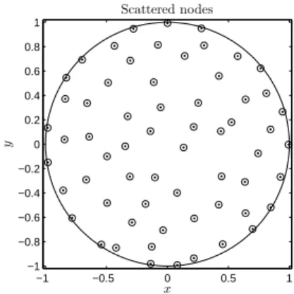
−1 −0.5 0 0.5 1 −1 −0.8 −0.6 −0.4 −0.2 0 0.2 0.4 0.6 0.8 1 x y Scattered nodes
Figure 2: Example ofN= 62 scattered nodes{ˆxj}Nj=1over the unit circle.
a vast amount of numerical cancellation will then arise when theO(1)-sized quantitys(x, ε) is computed in (1). This immediate numerical implementation of (2) followed by (1) is known as the RBF-Direct approach. It consists of two successive ill-conditioned numerical steps for obtaining a well-behaved quantity. Like the RBF-CP, RBF-QR, and RBF-GA algorithms, the new RBF-RA method computes exactly the same quantity s(x, ε) by following steps that all remain numerically stable even in theε→0 limit. The condition numbers of the linear systems that arise within all these algorithms remain numerically reasonable even whenε→0. This often highly accurate parameter regime therefore becomes fully available for numerical work.
One strategy that has been attempted for coping with the ill conditioning of RBF-Direct is to increase εwith N. If one keeps α=ε/N1/d constant ind-D, cond(A(ε)) stays roughly the same whenN increases.
However, this approach causes stagnation (saturation) errors [31, 34–36], which severely damage the
con-vergence properties of the RBF interpolant (and, for GA-type RBFs, causes concon-vergence to fail altogether). While convergence can be recovered by appending polynomial terms, it is reduced from spectral to algebraic.
3. Vector-valued rational approximation
The goal in this section is to keep the discussion of the vector-valued rational approximation method rather general since, as demonstrated in [37], it can be effective also for non-RBF-type applications. Let
f(ε) :C→ CM (withM > 1) denote a vector-valued function with componentsfj(ε),j = 1, . . . , M, that
are analytic at all points within a region Ω around the origin of the complex ε-plane except at possibly a finite number of isolated singular points (poles). Furthermore, suppose thatf has the following properties:
(i) AllM-components off share the same singular points.
(ii) Direct numerical evaluation off is only possible for|ε| ≥εR>0, where|ε|=εR is within Ω.
εR
Re(ε) Im(ε)
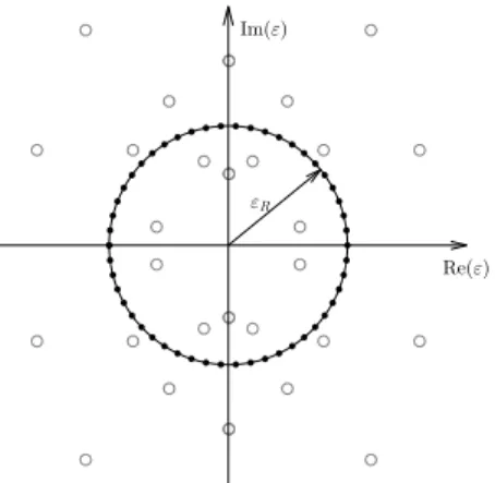
Figure 3: Schematic of the analytic nature of the vector-valued functionsf(ε) applicable to our vector-valued rational approxi-mation method. The small open disks show the location of the poles common to all components off(taken here to be symmetric about the axes). Solid black disks mark the locations wheref can be evaluated in a numerically stable manner. The goal is to use these samples to construct a vector-valued rational approximation of the form (4) that can be used to accurately compute
f for|ε|< εR.
We are interested in developing a vector-valued rational approximation to f that exploits these properties
and can be used to approximatef for allε < εR; see Figure 3 for a representative scenario. In Section 4, we
return to RBFs and discuss how these approximations are especially applicable to the stable computation
of RBF interpolation and RBF-FD/HFD weights, both of which satisfy the properties (i)–(iii), for smallε.
An additional property satisfied by these RBF applications is: (iv) The function f is even, i.e. f(−ε) =f(ε).
To simplify the discussion below, we will assume this property as well. However, the present method is easily adaptable to the scenarios where this is not the case, and indeed, also to the case that property (iii) does not hold.
We seek to find a vector-valued rational approximationr(ε) tof(ε) with components taking the form
rj(ε) =
a0,j+a1,jε2+a2,jε4+. . .+am,jε2m
1 +b1ε2+b2ε4+. . .+bnε2n
, j= 1, . . . , M. (4)
It is important to note here that only the numerator coefficients depend onj while the denominator coeffi-cients are independent ofjto exploit property (i) above. Additionally, we normalize the constant coefficient to one to match assumption (iii) and assume the numerators and denominator are even to match the as-sumption (iv). To determine these coefficients, we first evaluate f(ε) around a circle of radius ε=εR (see
Figure 3), wheref can be numerically evaluated in a stable manner. Due to assumption (iv), this evaluation only needs to be done at K points ε1, . . . , εK along the circle in the upper half-plane. We then enforce
that rj(ε) agrees with fj(ε) for all K evaluation points to determine all the unknown coefficients of r(ε).
The enforcement of these conditions can, for each j, be written as the following coupled linear system of
equations: 1 ε2 1 · · · ε 2m 1 1 ε2 2 · · · ε 2m 2 .. . ... . .. ... 1 ε2 K · · · ε2Km | {z } E a0,j .. . am,j | {z } aj + −diag(fj) ε2 1 · · · ε 2n 1 ε2 2 · · · ε 2n 2 .. . . .. ... ε2 K · · · ε2Kn | {z } Fj b1 .. . bn | {z } b = f(ε1) f(ε2) .. . f(εK) | {z } fj . (5)
=
0
0
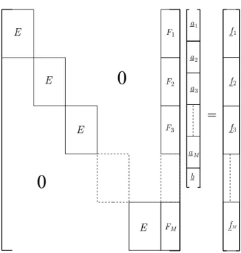
E F1 F2 F3 FM a1 a2 a3 aM b f1 f2 f3 fM E E EFigure 4: Structure of overdetermined linear system (5) for calculating the coefficients in the rational approximations (4).
coefficients corresponding to the different numerators ofr(ε) andn unknown coefficients corresponding to the one common denominator of r(ε). Since each subsystem in (5) is of sizeK-by-K, the complete system is of sizeKM-by-((m+ 1)M +n). We select parameters such thatm+ 1 +n/M < K so that the system is overdetermined.
A schematic of the efficient algorithm we use to solve this coupled system is displayed in Figure 5. Below are some details on the five steps of this algorithm:
Step 1: If an evaluation of f at some εk happens to have been at or near a pole, then there may be an
exceptionally large row in each Fj matrix and corresponding row of fj. For square linear systems,
multiplying a row by a constant will have no bearing on the system solution. However, for least squares problems, it will influence the relative importance associated with the equation. For eachεk, we thus
normalize each of the associated rows (inE,Fj, andfj) by dividing them bykf(εk)k∞to reduce their
inflated importance in the system. After this normalization, we compute a QR factorization of the
(modified)E matrix.
Step 2: We left multiply the system by a block-diagonal matrix with blocks Q∗ on the diagonal. This leaves
the same upper triangularRon the main diagonal blocks, withQ∗F
j in last column of block matrices
andQ∗f
j in the right hand side blocks.
Step 3: Starting from the top block equation, we re-order the rows so that the equations from the previous
step corresponding to the zero rows of R appear at the bottom of the linear system. This gives an
almost upper triangular system, with a full matrix block of sizeM(K−(m+ 1))-by-nin the last block
column, which we denote by ˙F, and the corresponding rows of the right hand side, which we denote
by ˙f.
Step 4: We compute the least squares solution to theM(K−(m+ 1))-by-noverdetermined system ˙F b= ˙f for the coefficients of the common denominator of the vector-valued rational approximation.
Step 1: Normalize large rows among all block
equations and compute aQRfactorization ofE.
Step 2: Multiply each block equation byQ∗.
=
0
0
QR F1 F2 F3 FM a1 a2 a3 aM b f1 f2 f3 fM QR QR QR=
0
0
R Q*F1 Q*F2 Q*F3 Q*FM R R R a1 a2 a3 aM b Q*F1 Q*f1 Q*f2 Q*f 3 Q*fMStep 3: Re-order the rows so no zero-rows lie in the blocks on the diagonal.
Step 4: Solve the decoupled, overdetermined system forb using least squares.
=
0
0
R R R R a1 a2 a3 b ⌅ ⇧ aM=
⇥
bStep 5: Solve the remainingM systems from Step 3 foraj using bfrom Step 4.
=
-R
a
jb
Figure 5: Algorithm and schematic diagram for solving the system in Figure 4. Note that in the actual implementation, one does not actually need to construct the whole linear system and only one copy ofQandRis kept.
coefficientsaj,j= 1, . . . , M. These systems are decoupled and consist of the same (m+ 1)-by-(m+ 1)
upper triangular block matrixR.
A Matlabimplementation of the entire vector-valued rational approximation method described above is
given in Appendix A, but with one modification that is applicable to RBFs. We assume that f(ε) =f(ε), which additionally impliesfis real whenεis real. This latter condition can be enforced onrby requiring that the coefficients in the numerators and single denominator are all real. Using this assumption and restriction on the coefficients of r, it then suffices to do the evaluations only along the circle of radiusεR in the first
quadrant and then split the resultingK/2 rows of the linear system (5) into their real and imaginary parts to obtainKrows that are now all real. This allows the algorithm in Figure 5 to work entirely in real arithmetic. The following are the dominant computational costs in computing the vector-valued rational approxima-tion:
1. computingfj(εk),j= 1, . . . , M, andk= 1, . . . , K,(ork= 1, . . . , K/2,in the case that the coefficients
are enforced to be real);
2. computing theQRfactorization ofE, which requiresO(K(m+ 1)2) operations;
3. computingQ∗F
j,j= 1, . . . , M, which requiresO(M Kmn) operations;
4. solving the overdetermined system forb, which requiresO(M(K−(m+ 1))n2) operations; and
5. solving the M upper triangular systems foraj, j= 1, . . . , M, which requiresO(M(m2+mn))
opera-tions.
We note that all of the steps of the algorithm are highly parallelizable, except for solving the overdetermined linear system for b. Additionally, we note that in cases where M is so large that it dominates the cost, it may be possible to just use a subset of the evaluation points to determineb, and then use these values to determine all of the numerator coefficients.
In addition to choosing the radius of the contour εR for evaluatingf, one also has to choose m,n, and
K in vector-valued rational approximation method. We discuss these choices as they pertain specifically to
RBF applications in the next section.
Remark 1. While we described the vector-valued rational approximation algorithm in terms of evaluation on a circular contour, this is not necessary. It is possible to use more general evaluation contours, or even evaluation locations that are scattered within some band surrounding the origin wheref can be evaluated in a stable manner.
4. RBF-RA method
In this section, we describe how the vector-valued rational approximation method can be applied to both computing RBF interpolants and to computing RBF-FD/HFD weights. We refer to the application of the vector-valued rational approximation method as the RBF-RA method. We focus first on RBF interpolation since the insights gleaned here can be applied to the RBF-FD/HFD setting (as well as many others).
4.1. Stable computations of RBF Interpolants
Before the RBF-CP method was introduced, ε was in the literature always viewed as a real valued
quantity. However, all the entries of the A(ε)-matrix, as given by (3), are analytic functions of ε and, in
the case of the GA kernel, they are entire functions of ε. Thus, apart from any singularities associated
with the kernelφthat is used to construct the interpolant, the entries ofA(ε)−1can have no other types of
singularities than isolated poles.
To illustrate the behavior of cond(A(ε)) in the complex plane, consider the N = 62 nodes {xˆi}Ni=1
scattered over the unit circle in Figure 2 and the GA kernel. For this example, pd(N) in Figure 1 is given
(a) (b)
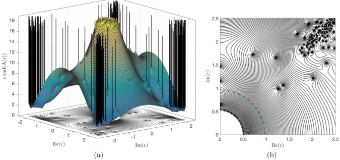
Figure 6: (a) Surface plot of log10cond(A(ε)) for the GA RBF and theN = 62 nodes displayed in Figure 2 together with a contour plot with 51 equally spaced contours from 1 to 17. (b) Contour plot of the surface in (a) over the first quadrant of the complexε-plane, now with 101 equally spaced contours from 1 to 17. The dashed line marks a typical path along which the RBF-RA algorithm performs its RBF-Direct evaluations.
holds also that||A(ε)−1||
2=O(ε−20). Figure 6 (a) shows a surface plot of log10(cond(A(ε))) in the complex
ε-plane. The first thing we note in this figure is that cond(A(ε)) is symmetric with respect to both the real and the imaginary axes since the interpolant (1) satisfies the symmetry relationship
s(x, ε) =s(x,−ε) =s(x, ε) =s(x,−ε). (6)
We also recognize the fast growth rate of cond(A(ε)) not only forε→0 along the real axis, but also when
ε →0 from any direction in the complex plane. Finally, we note sharp spikes corresponding to the poles
ofA(ε)−1. To illustrate the behavior of cond(A(ε)) further, we display a contour plot of log
10(cond(A(ε)))
in Figure 6 (b), but now only in the first quadrant, which is all that is necessary because of the symmetry conditions (6). The number of poles is seen to increase very rapidly with increasing distance from the origin,
but there are only a few present near the origin. The dashed line in Figure 6 (b) with radius 0.96 marks
where, in this case cond(A(ε))≈1012, which is an acceptable level for computings(x, ε) using RBF-Direct.
Now suppose that we are given M >1 points{xj}Mj=1 to evaluate the interpolants(x, ε) at, with εleft
as a variable. We can write this as the following vector-valued function ofε: s(x1, ε) s(x2, ε) .. . s(xM, ε) | {z } s(ε) = φε(kx1−ˆx1k) · · · φε(kx1−xˆNk) φε(kx2−ˆx1k) · · · φε(kx2−xˆNk) .. . . .. ... φε(kxM −xˆ1k) · · · φε(kxM −ˆxNk) | {z } Φ(ε) A(ε)−1 g1 .. . gN | {z } g . (7)
The entries of Φ(ε) are analytic functions of ε within some disk of radius εR centered at the origin and
A(ε)−1 can have at most poles in this disk. Thus, s(ε) in (7) is analytic inside this disk apart from the
poles of A(ε)−1. Furthermore, since each entry of s(ε) is computed from A(ε)−1, they all share the same
poles (note the similarity between Figure 6 (b) and Figure 3). Finally, we know that typically, and always in the case that the GA kernel is used, that ε = 0 must be a removable singularity of s(ε) [5, 7]. These observations together with the symmetry relationship (6), show that s(ε) satisfies all but possibly one of
the properties for the vector-valued functions discussed in the previous section that the new vector-valued rational approximation is applicable to.
The property that may not be satisfied by s(ε) is (ii). The issue is that the region of ill-conditioning of A(ε), which tends to be disk-shaped, may spread out so far in the complexε-plane that it is not possible
to find a radiusεR for the evaluation contour where RBF-Direct can be used to solve (7) or that does not
enclose the singular points associated with the kernels (branch points in the case of the MQ kernel and poles in the case of the IQ kernel). The GA kernel has no singular points. However, since it grows likeO(exp(|ε|2))
when π/4 <Arg(ε)< 3π/4, this leads to a different type of ill-conditioning in A(ε) in these regions (see
Figure 6) and prevents a radius that is too large from being used. ForN.100 in 2-D andN .300 in 3-D,
the region of ill-conditioning surroundingε= 0 is typically small enough (in double precision arithmetic) for a safe choice ofεR. As mentioned in the introduction, these limitations onN are not problematic in many
RBF applications. We discuss some strategies for choosingεRin Appendix B.
After choosing the radiusεRof the evaluation contour to use in the vector-valued rational approximation
method for (7), one must choose values form,n, andK. The optimal choice of these parameters depends on many factors, including the locations of the singular points fromA(ε)−1, which are not knowna priori. We
have found that for a givenK, choosingm=K−1−nandn=bK/4cgives consistently good results across the problems we have tried. With these choices, one can work out that the cost of the RBF-RA method
is O(KN(N2+M) +M K3). As demonstrated by the numerical results in Section 5, the approximations
converge rapidly withK, so that not too large a value ofKis required to obtain an acceptable approximation. With these parameters selected, we can construct a vector-valued rational approximationr(ε) fors(ε) in (7) that can be used as a proxy for computing the RBF interpolant stably for all values ofε inside the disk of radiusεR, includingε= 0.
4.2. Stable computations of RBF-FD and RBF-HFD formulas
RBF-FD and RBF-HFD formulas generalize standard, polynomial-based FD and compact or Hermite FD (HFD) formulas, respectively, to scattered nodes. We discuss here only briefly how to generate these formulas and how they can be computed using the vector-valued rational approximation scheme from Section 3. More thorough discussions of the RBF-FD methods can be found in [14], and more details on RBF-HFD methods can be found in [13].
Let Dbe a differential operator (e.g. the Laplacian) and ˆX ={xˆi}Ni=1 denote a set of (scattered) node
locations inRd. Supposeg:Rd→Ris some (sufficiently smooth) function sampled on ˆX and that we wish to approximateDg(x) atx=ˆx1 using a linear combination of samples ofg at the nodes in ˆX, i.e.
Dg(x) x=xˆ 1≈ N X i=1 wig(ˆxi). (8)
The RBF-FD method determines the weights wi in this approximation by requiring that (8) be exact
wheneverg(x) =φε(kx−ˆxik),i= 1, . . . , N, whereφεis, for example, one of the radial kernels from Table
1.1 These conditions can be written as the following linear system of equations:
A(ε) w1(ε) w2(ε) .. . wN(ε) | {z } w(ε) = Dxφε(kx−ˆx1k) x=xˆ 1 Dxφε(kx−ˆx2k) x=xˆ 1 .. . Dxφε(kx−ˆxNk)x=ˆx 1 | {z } Dxφε , (9)
1The RBF-FD (and HFD) method is general enough to allow for radial kernels that are not analytic functions ofε, or that do not depend on a shape parameter at all [31]. We assume the kernels are analytic in the presentation as the RBF-RA algorithm is applicable only in this case.
whereA(ε) is the standard RBF interpolation matrix with entries given in (3) andDxmeansDapplied with respect tox(this latter notation aids the discussion of the RBF-HFD method below). We have here explicitly marked the dependence of the weightswionε. Using the same arguments as in the previous section, we see
that the vector of weightw(ε) can be viewed as a vector-valued function ofεwith similar analytic properties
as an RBF interpolant based onφε. We can thus similarly apply the vector-valued rational approximation
algorithm for computingw(ε) in a stable manner as ε→0.
The additional constraint that (8) is exact whengis a constant is often imposed in the RBF-FD method,
which is equivalent to requiringPN
i=1wi=D1. This leads to an equality constrained quadratic programing
problem that can be solved using Lagrange multipliers leading to the following slightly modified version of the system in (9) for determiningw(ε):
A(ε) e eT 0 w(ε) λ(ε) = Dxφε D1 , (10)
where eis the vector of sizeN containing all ones, andλ(ε) is the Lagrange multiplier. The vector-valued rational approximation algorithm is equally applicable to approximatingw(ε) in this equation.
The HFD method is similar to the FD method, except that we seek to find an approximation ofDg(x) at
x=ˆx1that involves a linear combination ofg at the nodes in ˆX and a linear combination ofDgat another
set of nodes ˆY ={yˆj}Lj=1, i.e.
Dg(x) x=ˆx 1≈ N X i=1 wig(ˆxi) + L X j=1 ˙ wjDg(x) x=ˆy j. (11)
Here ˆx1 ∈/ Yˆ, or else the approximation is trivial, also ˆY is typically chosen to be some subset of ˆX (not
includingˆx1), but this is not necessary. The RBF-HFD method from [13] determines the weights by requiring
that (11) is exact forg(x) =φε(kx−ˆxik), i= 1, . . . , N, in addition tog(x) =Dyφε(kx−yk)
y=ˆy
j, where DymeansDapplied to the variabley. This givesN+Lconditions for determining the weights in (11). We can write these conditions as the following linear system for the vector of weights:
A(ε) B(ε) B(ε)T C(ε) | {z } ˜ A(ε) w(ε) ˙ w(ε) | {z } ˜ w(ε) = Dxφε DxDyφε , (12) where ˜w(ε) = w1(ε) · · · wN(ε) w˙1(ε) · · · w˙L(ε) T
,A(ε) is the standard interpolation matrix for the nodes in ˆX (see (3)), (B(ε))ij =Dyφ(kxi−yk) y=ˆy j, i= 1, . . . , N, j= 1, . . . , L, (C(ε))ij =Dx Dyφ(kx−yk) y=ˆy j x=ˆx i, i= 1, . . . , L, j= 1, . . . , L,and (DxDyφε)i=Dx Dyφ(kx−yk)y=ˆy i x=ˆx 1, i= 1, . . . , L.
The system (12) is symmetric and, under very mild restrictions on the operator D, is non-singular for all
the kernelsφεin Table 1; see [38] for more details.
Similar to the RBF-FD method, the vector of weights ˜w(ε) in (12) is an analytic vector-valued function ofεwith each entry sharing the same singular points, due now to ˜A(ε)−1, in a region surrounding the origin.
We can thus similarly apply the vector-valued rational approximation algorithm for computing ˜w(ε) in a
stable manner asε→0.
We note that in the RBF-HFD method it is also common to enforce that (11) is exact for constants. This constraint can be imposed in a likewise manner as the RBF-FD case in (10). We thus skip the details and refer the reader to [13] for the explicit construction.
0 0.2 0.4 0.6 0.8 1 ε 10-6 10-4 10-2 100
Relative max norm error
0 0.1 0.2 0.3 0.4 ε 10-6 10-4 10-2 100
Relative max norm error
0 0.1 0.2 0.3 0.4 ε 10-6 10-4 10-2 100
Relative max norm error
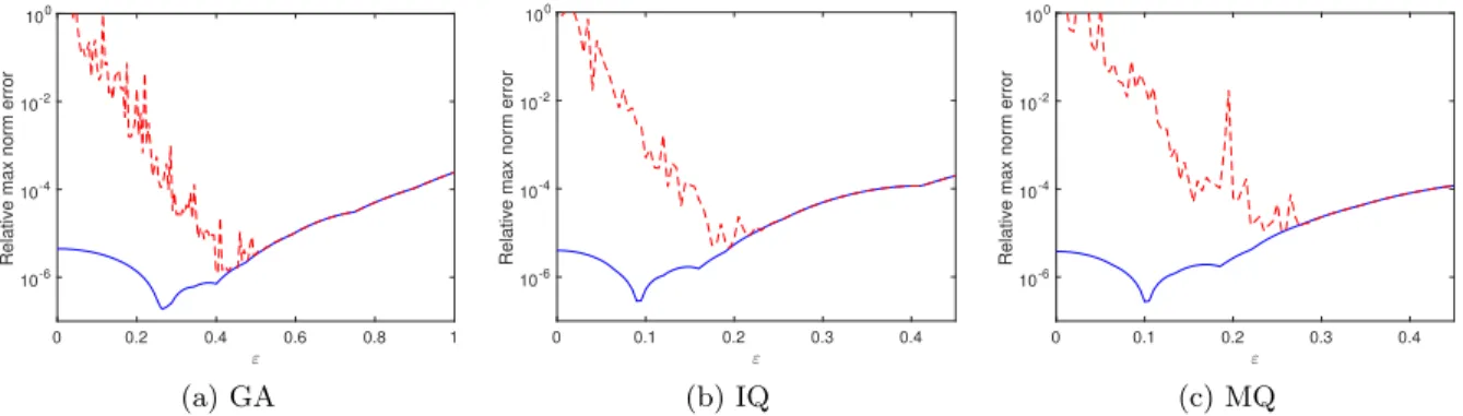
(a) GA (b) IQ (c) MQ
Figure 7: Comparison of the relative errors (computed interpolant−target function (13)) vs.εusing RBF-Direct (dashed lines) and RBF-RA (solid lines). Note the different scale on the horizontal axis in (a).
Remark 2. In using the vector-valued rational approximation algorithm for RBF applications, we have found that it is beneficial to spatially re-scale the node sets by the radius of the evaluation contour in the complex ε-plane, which allows all evaluations and subsequent computations of the algorithm to be done on the unit circle. This is the approach we follow in the examples given in Appendix A.
5. Numerical results
In this section, we first present results of the RBF-RA algorithm as applied to RBF interpolation and follow this up with some results on computing RBF-HFD formulas and their application to a ‘large-scale’ problem. The primary studies of the accuracy and robustness of the algorithm in comparison to the RBF-CP method and multiprecision arithmetic are given for RBF interpolation as the observations made here also carry over to the RBF-HFD setting.
5.1. RBF Interpolation results
Unless otherwise noted, all numerical results in this subsection are for the N = 62 nodes over the unit
disk shown in Figure 2 and for the target function g(x) =g(x, y) = (1−(x2+y2)) sinπ 2(y−0.07) −1 2cos π 2(x+ 0.1) . (13)
We useM = 41 evaluation pointsX ={xj}Mj=1 scattered over the unit disk in the RBF-RA algorithm and
also use these points to measure errors in the interpolant at various values ofε.
5.1.1. Errors between interpolant and target function
In the first numerical experiment, we compare the relative error in the RBF interpolant of the target function (13) using RBF-Direct and RBF-RA over a range of differentε. Specifically, we compute the relative error as
max
1≤j≤M|s(xj, ε)−g(xj)|/1≤maxj≤M|g(xj)|, (14)
for s computed with the two different techniques. The results are shown in Figure 7(a)-(c), for the GA,
IQ, and MQ radial kernels, respectively. We see that RBF-Direct works well for all these kernels until ill-conditioning of the interpolation matrices sets in, while RBF-RA allows the interpolants to be computed in
a stable manner right down toε= 0. The observed pattern of a dip in the RBF-RA error plots is common
and is explained in [6, 33]; it is a feature of the RBF interpolant and does not have to do with ill-conditioning of the RBF-RA method.
5.1.2. Accuracy vs. εandK
In all the remaining subsections of 5.1 except the last one, we focus on the difference between the computed interpolant and the exact interpolant. Specifically, we compute
max
1≤j≤M|s(xj, ε)−sexact(xj, ε)|/1≤maxj≤M|sexact(xj, ε)|, (15)
wheresis the interpolant obtained from either RBF-RA, RBF-CP, or RBF-Direct, andsexactis the ‘exact’
interpolant, computed using multiprecision arithmetic with 200 digits. Additionally, for brevity, we limit the presented results to the GA kernel as similar results were observed for other radial kernels.
0 0.2 0.4 0.6 0.8 1 ε 10-12 10-11 10-10 10-9 10-8 10-7 10-6 10-5
Relative max norm error
RBF-Direct RBF-CP RBF-RA 0 0.2 0.4 0.6 0.8 1 ε 10-12 10-11 10-10 10-9 10-8 10-7 10-6 10-5
Relative max norm error
RBF-Direct RBF-CP RBF-RA (a)K/2 = 22 (b)K/2 = 32 10 20 30 40 50 60 K/2 10-10 10-9 10-8 10-7 10-6 10-5 10-4 10-3 10-2
Relative two-norm error
RBF-CP
RBF-RA
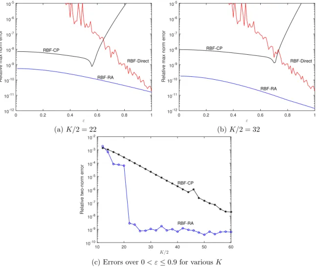
(c) Errors over 0< ε≤0.9 for variousK
Figure 8: Comparison of the errors (computed interpolant−exact interpolant) as the number of evaluations pointsKon the contour varies. Figures (a) and (b) show the relative max-norm error forε∈[0,1] forK/2 = 22 andK/2 = 32 (we useK/2 since this is this is the actual number of evaluations of the interpolant that are required). Figure (c) shows the relative two norm of the error taken only over 0≤ε≤0.9 as a function ofK/2.
In the first round of experiments, we compare the accuracy of the RBF-RA and RBF-CP algorithms as
a function of ε and K (the number of ε points on the contour used in both algorithms). We present the
results in terms ofK/2 since this is the actual total number of evaluations of the interpolants that have to be made (see comment towards the end of Section 3), which is the dominating cost of the algorithm. Figure 8 (a) shows the relative errors in the interpolants computed using the RBF-RA and RBF-CP methods for
0< ε≤1 and for K/2 = 22 andK/2 = 32, respectively. It is immediately obvious from these results that
asεgrows. Additionally, increasingK has only a minor effect on the accuracy of the RBF-RA method, but
has a more pronounced effect on the RBF-CP method, with an increased range ofεfor which it is accurate.
We explore the connection between accuracy and K further by plotting in Figure 8 (c) the relative errors
in the interpolant for many different K. Here the errors are computed for eachK, by first computing the
max-norm error (15) and then computing the two-norm of these errors over 0< ε≤0.9. We see that the
RBF-RA method converges rapidly withK, while the RBF-CP method converges much slower (but still at
a geometric rate). The reason the error stops decreasing in the RBF-RA method around 10−9 is that this
is about the relative accuracy that can be achieved using RBF-Direct to compute the interpolants on the contour in the complexε-plane.
5.1.3. RBF-RA vs. Multiprecision RBF-Direct
An all too common way to deal with the ill-conditioning associated with flat RBFs is to use multiprecision
floating point arithmetic with RBF-Direct. While this does allow one to consider a larger range of ε in
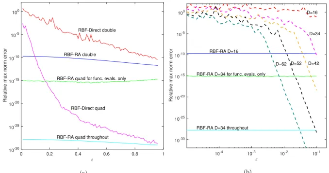
applications, it comes at a higher computational cost as the computations have to be done using special software packages instead of directly in hardware. Typically, quad precision (approximately 34 decimal digits) is used since floating point operations on these numbers can combine two double precision numbers, which can improve the cost. Figure 9 (a) compares the errors in the interpolants computed using RBF-RA and RBF-Direct with both double and quad precision arithmetic, with the latter being computed using
the Advanpix multiprecisionMatlabtoolbox [39]. We see from the figure that the range of εthat can be
considered with RBF-Direct and quad precision increases, but that the method is still not able to consider the full range. There is nothing to prevent quad precision from also being used with RBF-RA and in Figure 9 (a) we have included two results with quad precision. The first uses quad precision only to evaluate the interpolant (which is the step that has the potential to be ill-conditioned), with all subsequent computations of the RA method done in double precision. The second uses quad precision throughout the entire RBF-RA algorithm. We see from the results that the errors in the interpolant for both cases are now much lower than the double precision case. In Figure 9 (b) we further explore the use of multiprecision arithmetic with the RBF-Direct algorithm (again using Advanpix) by looking at the error in the interpolant as the number of digits used is increased. Now, we consider 10−5 < ε≤10−1 to clearly illustrate that the ill-conditioning
of RBF-Direct cannot be completely overcome with this technique, but that it can be completely overcome with RBF-RA.
5.1.4. Contours passing close to poles
To demonstrate the robustness of the new RBF-RA algorithm we consider a case where the evaluation contour runs very close to a pole in the complexε-plane. For theN = 62 node example we are considering in these numerical experiments, there is a pole atε≈1.4617904771448i. We choose for both the RBF-RA and RBF-CP algorithms a circular evaluation contour centered at the origin of radiusεR= 1.4618. This contour
is superimposed on a contour plot of the condition number in Figure 10 (a) (see the dashed curve). Figure 10 (b) shows the max-norm errors (again together with RBF-Direct for comparison) in the interpolants (15) computed with both algorithms using this contour. We see that the RBF-CP algorithm gives entirely useless results for this contour, while the RBF-RA algorithm performs as good (if not slightly better) than the case where the contour does not run close to any poles.
5.1.5. Vector-valued rational approximation vs. rational interpolation
A seemingly simpler approach to obtain vector-valued rational approximations to the interpolant s(ε)
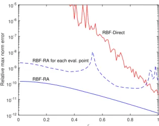
in (7) is to use rational interpolation (or approximation) of each of the M entries of s(ε) separately [40], instead of the RBF-RA procedure that couples the entries together. However, we have found that this does not produce as accurate results and can lead to issues with the approximants. Figure 11 illustrates this by
comparing the errors that result from approximatingsusing the standard RBF-RA procedure to that of using
RBF-RA separately for each of theM entries ofs(ε) (which amounts to computing a rational interpolant of each entry). We first see from this figure that the RBF-RA procedure is at least an order of magnitude more accurate than the rational interpolation approach. Second, we see a few values ofεwhere the error spikes in
0 0.2 0.4 0.6 0.8 1 ε 10-30 10-25 10-20 10-15 10-10 10-5 100
Relative max norm error
RBF-Direct double
RBF-RA double
RBF-RA quad for func. evals. only
RBF-Direct quad
RBF-RA quad throughout
(a) 10-4 10-3 10-2 10-1 ε 10-30 10-25 10-20 10-15 10-10 10-5 100
Relative max norm error
D=16 D=34 D=42 D=52 D=62 RBF-RA D=16
RBF-RA D=34 for func. evals. only
RBF-RA D=34 throughout
(b)
Figure 9: (a) Comparison of the errors (computed interpolant−exact interpolant) using double precision and quad precision arithmetic. The top RBF-RA quad curve corresponds to using quad precision only when evaluating the interpolant, whereas the bottom quad curve corresponds to using quad precision for all the computations in the RBF-RA method. (b) Similar to (a) but for multiple precision arithmetic using D digits (here D=16 is double precision and D=34 is quad precision). Here RBF-Direct results are in the dashed lines; note also the logarithmic scale inε.
0 0.2 0.4 0.6 0.8 1 ε 10-12 10-10 10-8 10-6 10-4 10-2 100 102 104
Relative max norm error
RBF-Direct RBF-CP
RBF-RA
(a) (b)
Figure 10: (a) Contour plot of log10(cond(A(ε))) (similar to Figure 6 (b)) with an evaluation contour (dashed line) running very close to a pole on the imaginary axis. (b) Comparison of the errors (computed interpolant−exact interpolant) associated with the RBF-RA and RBF-CP algorithms using the evaluation contour in part (a). Here we usedK/2 = 32 evaluation points on the contour; doubling this number does not appear to improve the RBF-CP results at all.
0 0.2 0.4 0.6 0.8 1 ε 10-12 10-11 10-10 10-9 10-8 10-7 10-6 10-5
Relative max norm error
RBF-Direct
RBF-RA for each eval. point
RBF-RA
Figure 11: Comparison of the errors (computed interpolant−exact interpolant) when using RBF-RA with all the evaluation points (solid line marked RBF-RA), when applying RBF-RA separately to each evaluation point (dashed line), and when using RBF-Direct. In the second case, a rational approximant is computed separately for each entry of the vector-valued function. In both RBF-RA cases, we setK/2 = 40.
the rational interpolation method. These spikes correspond to spurious poles, or “Froissart doublets” [41],
appearing near or on the real ε-axis. Froissart doublets are especially common in rational approximation
methods where the input contains noise [42], which occurs in our application at roughly the unit roundoff of the machine times the condition number of the RBF interpolation matrix on the evaluation contour of the RBF-RA algorithm. The least squares nature of determining a common denominator in the RBF-RA method appears to significantly reduce the presence of these spurious poles. In fact, we have not observed the presence of Froissart doublets in any of our experiments with RBF-RA.
5.1.6. Timing example for a 3-D problem
Finally, we compare the computational cost of the RBF-RA method to that of the RBF-Direct method. For this comparison, we use Halton node sets over the unit cube inR3of increasing sizeN (generated with theMatlabfunctionhaltonset). For the evaluation points, we also use Halton node sets with the same
cardinality as the nodes (i.e. M =N), but shift them so they don’t agree with the nodes; havingM =N
is a common scenario in generating RBF-FD/HFD formulas. The target functiong is not important in this
experiment, as we are only concerned with timings. Figure 12 (a) shows the measured wall clock times of two methods for evaluating the interpolant at ε = 10−2. Included in this figure are the wall clock times
also for computing the interpolants using multiprecision arithmetic, with D = 100 digits for RBF-Direct
and with D= 34 (quad precision) for RBF-RA. For theN >100 andε= 0.01, it is necessary to switch to multiprecision arithmetic with RBF-Direct to get a meaningful result, whereas RBF-RA in double precision has no issues with ill-conditioning. WhileD= 100 is larger than is necessary for RBF-Direct withε= 10−2,
it is reasonable for smallerε (see Figure 9 (b)), also the timings do not go down very much by decreasing
D. The quad precision results are included for comparison purposes with RBF-Direct in multiprecision
mode; they are not necessary to obtain an accurate result for these values ofN. For the double precision
computations, we see that the cost of RBF-RA is about 100 times that of RBF-Direct. However, for small
ε, the comparison should really be made between RBF-Direct using multiprecision arithmetic, in which case
RBF-RA is about an order of magnitude more efficient. Based on the timing results in [12, Section 6.3], the computational cost of the RBF-RA method is about a factor of two or three larger than the RBF-QR method and about a factor of ten larger than the RBF-GA method, which (at about 10 times the cost of RBF-Direct) is the fastest of the stable algorithms (for GA RBFs).
One added benefit of the RBF-RA method is that evaluating the interpolant at multiple values ofε(which is required for some shape parameter selection algorithms) comes at virtually no additional computational cost. The same is not true for the RBF-Direct method. We demonstrate this feature in Figure 12 (b), where
101 102 103 N 10-4 10-3 10-2 10-1 100 101 102 Runtime (s) RBF-Direct double RBF-RA double RBF-Direct 100 digits RBF-RA quad RBF-RA quad RBF-Direct 100 digits RBF-RA double RBF-Direct double
(a) One value ofε.
101 102 103 N 10-4 10-3 10-2 10-1 100 101 102 Runtime (s) RBF-Direct double RBF-RA double RBF-Direct 100 digits RBF-RA quad RBF-RA quad RBF-Direct 100 digits RBF-RA double RBF-Direct double (b) Ten values ofε.
Figure 12: Measured wall clock time (in seconds) as a function of the number of 3-D Halton nodesN for the RBF-RA (with K/2 = 32) and RBF-Direct methods. (a) A comparison of the methods for computing the interpolant atM =N evaluation points and for one value ofε(set toε= 10−2). (b) Same as (a), but for computing the interpolant at ten values ofε(set to
εj= 10−j,j= 0, . . . ,9). The dashed lines were computed using multiprecision arithmetic, withD= 100 digits for RBF-Direct
andD= 34 (quad precision) for RBF-RA. All timings were done usingMatlab2016a on a 2014 MacBook Pro with 16 GB of RAM and an 3GHz Intel Core i7 processor without explicit parallelization. The multiprecision computations were done using the Advanpix multiprecisionMatlabtoolbox [39].
the wall clock times of the algorithms are displayed for evaluating the interpolants atεj= 10−j,j= 0, . . . ,9.
The dominant cost of the RBF-RA method comes from evaluating the interpolant on the contour, which can be done in parallel. The timings presented here have made no explicit use of parallelization for these evaluations, so further improvements to the of efficiency the method over RBF-Direct are still possible.
5.2. RBF-HFD results
In this section we consider the application of the RBF-RA method to computing RBF-HFD weights for the 3-D Laplacian and use these to solve Poisson’s equation in a spherical shell. Specifically, we are interested solving ∆u=g, in Ω =n(x, y, z)∈R3 0.55≤ p x2+y2+z2≤1o, (16)
subject to Dirichlet boundary conditions on the inner and outer surfaces of the shell. Here we take the exact solution to be u(λ, θ, r) = sin 20π 9 r−11 20 Y 0 6(λ, θ) + 14 11Y 5 6(λ, θ) , where (λ, θ, r) are spherical coordinates andYm
` denote real-valued spherical harmonics of degree`and order
m. This uis used to generateg in (16) to set up the problem. We use 500,000 global nodes to discretize the shell2; see the left image of Figure 13 for an illustration of the nodes. We denote the nodes interior to
the shell by Ξint ={ξ
k}Pk=1 and the nodes on the boundary by Ξ
bnd={ξ k}
P+Q
k=P+1. For our test problem,
P = 453,405 andQ= 46,595.
The procedure for generating the RBF-HFD formulas is as follows: Fork= 1, . . . , P repeat the following
2These nodes were generated by Prof. Douglas Hardin at Vanderbilt University using a modified version of the method discussed in[43].
1. Select theN−1 nearest neighbors ofξkfrom Ξint∪Ξbnd(using ak-d tree for efficiency), withN << P.
These nodes plusξk form the set ˆX ={ˆxi}Ni=1 in (11), with the convention thatˆx1=ξk.
2. From the set ˆX, select theL < N nearest-neighbors to ˆx1. These nodes form the set ˆY ={yˆj}Lj=1 in
(11).
3. Use ˆX, ˆY, and D = ∆ in (12), then apply the vector-valued rational approximation algorithm to
compute the weights for given values of ε. Note that standard Cartesian coordinates can be used in
applyingDin (12) [21].
In the numerical experiments, we setN= 45 andL= 20 and use the IQ radial kernel. We also setK/2 = 64
and choosen=K/4.
We first demonstrate the accuracy of the RBF-RA procedure for computing the RBF-HFD weights in theε→0 limit by comparing the computed weights for one of the stencils to the ‘exact’ value of the weights
computed using multiprecision arithmetic withD = 200 digits. The results are displayed in Figure 14 (a),
together with the error in the weights computed with RBF-Direct in double precision arithmetic. We can see from the figure that the RBF-RA method can compute the weights in a stable manner for the full range ofε, with no loss in accuracy from the computation using RBF-Direct in the numerically ‘safe’ region.
Next, we use the RBF-HFD weights to numerically solve the Poisson equation (16) for various values of εin the interval [0,8]. Lettinguandg denote samples at the nodes Ξint of the unknown solution and right
hand side of (16), respectively, the discretized version of (16) can be written as
Du= ˙Dg.
In this equation, D and ˙D are two sparse P-by-P matrices with the kth row ofD containing the explicit
weightswi in (11) and thekth row of ˙Dcontaining the implicit weights ˙wj in (11), for the kth node of Ξint.
To solve this system, we used BiCGSTAB with a zero-fill ILU-preconditioner and a tolerance on the relative residual of 10−10. Figure 14 (b) shows the relative two-norm of the errors in the approximate solutions as
a function of ε. Marked on this plot is the region where RBF-Direct becomes unstable, and RBF-RA is
used. We see that a reduction of the error by nearly two orders of magnitude is possible for εvalues that
are untouchable with RBF-Direct in double precision arithmetic. We note that for all values ofε, the solver
required an average of 27.5 iterations and took 13.95 seconds of wall clock time usingMatlab2014b on a
Linux workstation with 96 GB of RAM and dual 3.1GHz 8-core Intel Xeon processors.
6. Concluding remarks
The present numerical tests demonstrate that the RBF-RA algorithm can be used effectively for stably
computing RBF interpolants and RBF-FD/HFD formulas in theε→0 limit. The method is more accurate
and computationally efficient than the Contour-Pad´e method, and more flexible than the QR and RBF-GA algorithms, in that operations such as differentiation can readily be applied directly to the RBFs instead of to the more complex bases that arise in these other two methods. Its main disadvantages compared to these methods are (i) that it is not quite as efficient, and (ii) that it is more limited in the node sizes it can handle. However, with the main target application of the algorithm being to compute RBF-FD and RBF-HFD formulas, these disadvantages are not serious concerns. The RBF-RA algorithm is also applicable to more general rational function approximation problems that involve vector-valued analytic functions with components that have the same singular points.
A known issue with the RBF-CP, RBF-GA, and RBF-QR method is that the accuracy degrades if the nodes lie on a portion of a lower dimensional algebraic curve or surface (e.g. a cap on the unit sphere inR3). This issue also extends to the RBF-RA method and will be a future topic of research.
−−−
−−−
−−−
−−−
→
Figure 13: Illustration of the global and local node set used in the RBF-HFD method for solving Poisson’s equation in a spherical shell with radius 0.55≤r≤1, which mimics the aspect radius of the Earth’s mantle. The left figure shows the shell split open, with part of the 5·105 global node set marked by small solid spheres. A small subset of the nodes is shown to the right, with the HFD stencil?s ‘center’ node marked in red.
0 1 2 3 4 5 6 7 8 ε 10-12 10-10 10-8 10-6 10-4 10-2 100 102
Relative max norm error
RBF-Direct RBF-RA 0 1 2 3 4 5 6 7 8 ε 10-7 10-6 10-5 10-4
Relative two norm error
RBF-Direct RBF-RA
(a) RBF-HFD weights (b) Solution to Poisson’s equation
Figure 14: (a) Comparison of the errors in the computation of the RBF-HFD weights for one of the stencils from the node set shown in Figure 13. The errors are measured against a multiprecision computation of the weights using 200 digits. (b) Relative two-norm of the error in solving Poisson’s equation (16) using RBF-HFD formulas as a function ofε. The dashed line marks the values ofεwhere RBF-Direct can be safely used to compute the RBF-HFD weights, while the solid line marks the values where RBF-RA is required to get an accurate result. The results in both plots were obtained usingN= 45 andL= 20.
Acknowledgments
The authors thank Nick Trefethen for many fruitful discussions regarding rational approximations when they were first putting the ideas of this paper together. The work of Grady Wright was supported by National Science Foundation grants DMS-1160379 and ACI-1440638.
Appendix A. Matlab Code and examples
This appendix contains first the script for two examples, followed by the functions rbfhfd, vvra, and
polyval2. The functionvvra (standing for vector-valued rational approximation) implements the general algorithm described in Section 3. The first example shows how to use thevvrafunction for RBF interpolation. The output of this example is a plot showing the maximum difference between the interpolant and the target function (13) as function of epsilon. It also displays the minimum of these maximum differences and the corresponding value ofε. These numbers are 2.82·10−7 and 0.31, respectively. The second example shows
how to use thevvrafunction for computing RBF-HFD weights. The code uses the standard 19 node compact
stencil for the 3-D Laplacian [44] and shows that the RBF-HFD weights in theε→0 limit are the same (up
to rounding errors) as the standard polynomials based weights. The output of this example is the relative two norm difference between and flat limit RBF-HFD weights and the standard weights. This number is 4.38·10−13.
%% Example 1: Interpolation problem using GA kernel
phi = @(e,r) exp(-(e*r).^2); % Gaussian
f = @(x,y) (1-(x.^2+y.^2)).*(sin(pi/2*(y-0.07))-0.5*cos(pi/2*(x+0.1))); N = 60; hp = haltonset(2); y = 2*net(hp,N)-1; % Nodes/centers
M = 2*N; x = 3/2*net(scramble(hp,’rr2’),M)-3/4; % Eval points
epsilon = linspace(0,1,101);
% Compute distances nodes/centers and eval points/centers
D = @(x,y)hypot(bsxfun(@minus,x(:,1),y(:,1)’),bsxfun(@minus,x(:,2),y(:,2)’)); ryy = D(y,y); rxy = D(x,y);
% Determine the radius
rad = fminbnd(@(e)norm(inv(phi(e,ryy)),inf)*norm(phi(1i*e,ryy),inf),0.1,20); ryy = ryy*rad; % Re-scale the distances by the radius of the evaluation
rxy = rxy*rad; % contour so that a unit radius can be used. % Compute the interpolant
rbfinterp=@(ep) phi(ep,rxy)*(phi(ep,ryy)\f(y(:,1),y(:,2))); s = vvra(rbfinterp,epsilon/rad,1,64,64/4);
% Compute the difference between s and f and plot the results
error = max(abs(bsxfun(@minus,s,f(x(:,1),x(:,2))))); semilogy(epsilon,error,’x-’)
[minerr,pos] = min(error);
fprintf(’Minimum error: %1.2e, Epsion: %1.2f\n’,minerr,epsilon(pos));
%% Example 2: RBF-HFD weights for the 3-D Laplacian using IQ kernel % Example for the standard 19 node stencil (6 implicit nodes) on lattice % Explicit nodes xhat = [[0,0,0];[-1,0,0];[1,0,0];[0,-1,0];[0,1,0];[0,0,-1];[0,0,1];... [0,-1,-1];[0,-1,1];[0,1,-1];[0,1,1];[-1,0,-1];[-1,0,1];... [1,0,-1];[1,0,1];[-1,-1,0];[-1,1,0];[1,-1,0];[1,1,0]]; N = size(xhat,1); % Implicit nodes
yhat = [[-1,0,0];[1,0,0];[0,-1,0];[0,1,0];[0,0,-1];[0,0,1]];
plot3(xhat(:,1),xhat(:,2),xhat(:,3),’o’,yhat(:,1),yhat(:,2),yhat(:,3),’.’)
% The IQ kernel and it’s 3-D Laplacian and 3-D bi-harmonic
phi = @(e,r) 1./(1 + (e*r).^2);
dphi = @(e,r) 2*e^2*(-3 + (e*r).^2)./(1 + (e*r).^2).^3;
d2phi = @(e,r) 24*e^4*(5 + (e*r).^2.*(-10 + (e*r).^2))./(1 + (e*r).^2).^5;
% Compute the radius
rad = fzero(@(e)log10(cond(rbfhfd(e,xhat,yhat,phi,dphi,d2phi,1)))-6,[0.05,1]); r = sqrt(D(xhat,xhat).^2 + bsxfun(@minus,xhat(:,3),xhat(:,3)’).^2);
rad = min(rad,0.95/max(r(:)));
% Re-scale the stencil nodes so that a unit evaluation radius can be used.
xhat = rad*xhat; yhat = rad*yhat;
% Compute the weights at various epsilon
epsilon = linspace(0,rad,11);
w = vvra(@rbfhfd,epsilon/rad,1,64,64/4,xhat,yhat,phi,dphi,d2phi);
% Undo the effects of re-scaling from the weights
w(1:size(xhat,1),:) = w(1:size(xhat,1),:)*rad^2;
% Compare the flat limit weights (epsilon=0) to the standard weights
ws = [-8,2/3*ones(1,6),ones(1,12)/3,-ones(1,6)/6]’; % standard weights
fprintf(’Relative two norm difference: %1.2e\n’,norm(w(:,1)-ws)/norm(ws));
function w = rbfhfd(ep,x,xh,phi,dphi,d2phi,flag)
%RBFHFD Computes the RBF-HFD weights for the 3-D Laplacian. %
% w = rbfhfd(Epsilon,X,Xh,Phi,DPhi,D2Phi) computes the RBF-HFD weights % at the given value of Epsilon and at the explicit stencil nodes X and % implicit (Hermite) stencil nodes Xh. Phi is a function handle for % computing the kernel phi(ep,r) used for generating the weights (e.g. % the Gaussian or inverse quadratic). Dphi and D2phi are function % handles for computing the 3-D Laplacian and bi-harmonic of Phi, % respectively.
%
% A = rbfhfd(Epsilon,X,Xh,Phi,DPhi,D2Phi,flag) returns the matrix for % computing the weights if the flag is non-zero, otherwise it returns % just the weights as described above.
if nargin == 6
flag = 0; % Return on the weights end
N = size(x,1); x = [x;xh];
ov = ones(1,size(x,1));
% Compute the pairwise distances
r = sqrt((x(:,1)*ov-(x(:,1)*ov).’).^2 + (x(:,2)*ov-(x(:,2)*ov).’).^2 + ...
(x(:,3)*ov-(x(:,3)*ov).’).^2);
temp = dphi(ep,r(1:N,N+1:end)); % Construct the weight matrix
A = [[phi(ep,r(1:N,1:N)) temp];[temp.’ d2phi(ep,r(N+1:end,N+1:end))]];
% Determine what needs to be returned. if flag == 0
w = A\[dphi(ep,r(1:N,1));d2phi(ep,r(N+1:end,1))];
else
end
end % end rbfhfd
function [R,b] = vvra(myfun,epsilon,rad,K,n,varargin)
%VVRA Vector-valued rational approximation (VVRA) valid near the % origin to a vector-valued analytic function.
%
% [R,b] = vvra(myfun,Epsilon,Rad,K,n) generates a vector-valued rational % approximation to the vector-valued analytic function represented by % myfun and evaluates it at the values in Epsilon. The inputs are % described as follows:
%
% myfun is a function handle that, given a value of epsilon returns a % column vector corresponding to each component of the function % evaluated at epsilon.
%
% Epsilon is an array of values such that |Epsilon|<=Rad where the % rational approximation is to be evaluated.
%
% Rad is a scalar representing the radius of the circle centered at % the origin where it is numerically safe to evaluate myfun.
%
% K is the number of points to evaluate myfun at on the contour for % constructing the rational approximation. This number should be even. %
% 2n is the degree of the common denominator to use in the % approximation.
%
% The columns in the output R represent the approximation to the % components of myfun at each value in the array Epsilon. The optional % output b contains the coefficients of the common denominator of the % vector-valued rational approximation.
%
% [R,b] = vvra(myfun,Epsilon,Rad,K,n,T1,T2,...) is the same as above, but % passes the optional arguments T1, T2, etc. to myfun, i.e.,
% feval(myfun,epsilon,T1,T2,...).
K = K+mod(K,2); % Force K to be even
ang = pi/2*linspace(0,1,K+1)’; ang = ang(2:2:K);
ei = rad*exp(1i*ang); % The evaluation points (all in first quadrant)
m = K-n; % Fix the degree of the numerator based on K and n
W = feval(myfun,ei(1),varargin{:}); M = numel(W);
fv = zeros(K/2,1,M); fv(1,1,:) = W;
for k = 2:K/2 % Loop over the evaluation points for F
W = feval(myfun,ei(k),varargin{:}); fv(k,1,:) = W;
end
fmax = max(abs(fv),[],3); % Find largest magnitude component for each k
e = ei.^2; % Calculate the E matrix
f = E(:,1:n+1); % Create the F-matrices and RHS
F = f(:,:,ones(1,M)).*fv(:,ones(1,n+1),:); g = F(:,1,:);
F = -F(:,2:n+1,:);
ER = [real(E);imag(E)]; % Separate E and F and the RHS g into real parts on
FR = [real(F);imag(F)]; % top, and then the imag parts below
gr = [real(g);imag(g)];
[Q,R] = qr(ER); QT = Q’; % Factorize ER into Q*R
R = R(1:m,:); % Remove bottom block of zeros from R for k = 1:M % Update all FR matrices
FR(:,:,k) = QT*FR(:,:,k); gr(:,1,k) = QT*gr(:,1,k);
end
FT = FR(1:m,:,:); % Separate F-blocks and g-blocks to the systems for
FB = FR(m+1:K,:,:); % determining the numerator and denominator coeffs.
gt = gr(1:m,:,:); gb = gr(m+1:K,:,:);
% Reshape these to be 2-D matrices
FT = permute(FT,[1,3,2]); FT = reshape(FT,M*m,n); FB = permute(FB,[1,3,2]); FB = reshape(FB,M*(K-m),n); gt = permute(gt,[1,3,2]); gt = reshape(gt,M*m,1); gb = permute(gb,[1,3,2]); gb = reshape(gb,M*(K-m),1);
b = FB\gb; % Obtain the coefficients of the denominator
v = gt-FT*b; V = reshape(v,m,M);
a = (R\V); % Obtain the coefficients of the numerators % Evaluate the rational approximations
R = zeros(M,length(epsilon)); b = [1;b]; denomval = polyval2(b,epsilon); for ii = 1:M R(ii,:) = (polyval2(a(:,ii),epsilon)./denomval); end
end % End vvra
function y = polyval2(p,x)
%POLYVAL2 Evaluates the even polynomial
% Y = P(1) + P(2)*X^2 + ... + P(N)*X^(2(N-1)) + P(N+1)*X^2N % If X is a matrix or vector, the polynomial is evaluated at all % points in X (this is unlike the polyval function of matlab)
y = zeros(size(x)); x = x.^2;
for j=length(p):-1:1 y = x.*y + p(j);
end
end % End polyval2
Appendix B. Choosing the radiusεR of the evaluation contour
We propose two different strategies for choosing the radius εR depending on the type of kernel being
used in the application. As discussed in Section 4.1, entire positive definite kernels, like GA, grow without
of the contour. The strategy we propose for entire kernels is to choose εR based on an estimate of where
the ill-conditioning from the interpolation problem is overtaken by ill-conditioning from the growth of the
kernel on the imaginary ε-axis. Such an estimate is difficult to make from the condition number of the
interpolation or RBF-FD/HFD weight matrix A(ε) because of singularities that can occur in A(ε)−1 for
imaginaryε (cf. Figure 6). Instead, we have found that a good measure for the ill-conditioning that is not effected by singularities whenε=iβ (β ∈R) is
e
σ∞(A(β)) =kA(iβ)k∞kA(β)−1k∞.
The first factor on the right of this expression captures the growth from the kernel, while the second factor captures the ill-conditioning from the interpolation problem (since this is just the standard interpolation matrix for real shape parameters). To find where the transition between the types of ill-conditioning occurs,
we thus set εR equal to an approximate minimum of logeσ∞(A(β)). This is the approach used in the
interpolation example in the first appendix.
As discussed in Section 4.1, kernels that have singular points, such as IQ, IMQ, and MQ, will lead to a multitude of singular points in the RBF vector-valued rational function, as each entry of A(ε) will have two singular points. The evaluation contour that is used should altogether avoid these singular points. The closest singular points that comes directly from the kernels is located on the positive and negative imaginary axis at the inverse of the largest distance between the nodes. The radiusεRthus needs to be chosen smaller
than this value. In our applications we have used εR= 0.95 max 1≤i,j,≤Nkˆxi−ˆxjk −1 , (B.1)
where {ˆxi}Ni=1 are the interpolation (or RBF-FD stencil) nodes. For smaller problems, we have found that
this sometimes results in a radius that is larger than necessary to achieve accurate results. In these case we often find it is better to use a smaller radius, which in turn allows the number of evaluation pointsKto be
smaller without diminishing the accuracy. To address this issue, we chooseεR to be the minimum between
(B.1) and the approximate real value of εwhere the condition number ofA(ε) is equal to 106. This is the
approach used in the RBF-HFD example in the first appendix.
References
[1] B. Fornberg, C. Piret, On choosing a radial basis function and a shape parameter when solving a convective PDE on a sphere, J. Comput. Phys. 227 (2008) 2758–2780.
[2] E. Larsson, B. Fornberg, A numerical study of some radial basis function based solution methods for elliptic PDEs, Comput. Math. Appl. 46 (2003) 891–902.
[3] R. Schaback, Error estimates and condition numbers for radial basis function interpolants, Adv. Comput. Math. 3 (1995) 251–264.
[4] T. A. Driscoll, B. Fornberg, Interpolation in the limit of increasingly flat radial basis functions, Comput. Math. Appl. 43 (3) (2002) 413–422.
[5] B. Fornberg, G. Wright, E. Larsson, Some observations regarding interpolants in the limit of flat radial basis functions, Comput. Math. Appl. 47 (2004) 37–55.
[6] E. Larsson, B. Fornberg, Theoretical and computational aspects of multivariate interpolation with increasingly flat radial basis functions, Comput. Math. Appl. 49 (2005) 103–130.
[7] R. Schaback, Multivariate interpolation by polynomials and radial basis functions, Constr. Approx. 21 (2005) 293–317.
![Figure 1: The functions p d (N ) in the condition number estimate cond(A(ε)) = O(ε −p d (N ) ) from [33] for d = 1, 2, 3](https://thumb-us.123doks.com/thumbv2/123dok_us/9234322.2808160/4.918.215.703.274.540/figure-functions-n-condition-number-estimate-cond-ε.webp)