04 August 2020
POLITECNICO DI TORINO
Repository ISTITUZIONALE
Mining and modeling web trajectories from passive traces / Vassio, Luca; Mellia, Marco; Figueiredo, Flavio; Couto da Silva, Ana Paula; Almeida, Jussara M.. - ELETTRONICO. - (2017), pp. 4016-4021. ((Intervento presentato al convegno 2017 IEEE International Conference on Big Data (BIGDATA) tenutosi a Boston (USA) nel 11-14 Dicembre 201.
Original
Mining and modeling web trajectories from passive traces
ieee Publisher: Published DOI:10.1109/BigData.2017.8258416 Terms of use: openAccess Publisher copyright
copyright 20xx IEEE. Personal use of this material is permitted. Permission from IEEE must be obtained for all other uses, in any current or future media, including reprinting/republishing this material for advertising or promotional purposes, creating .
(Article begins on next page)
This article is made available under terms and conditions as specified in the corresponding bibliographic description in the repository
Availability:
This version is available at: 11583/2697991 since: 2018-01-25T11:38:15Z
Mining and Modeling Web Trajectories
from Passive Traces
Luca Vassio, and Marco Mellia Politecnico di Torino
Torino, Italy
{luca.vassio, marco.mellia}@polito.it
Flavio Figueiredo, Ana Paula Couto da Silva, and Jussara M. Almeida Universidade Federal de Minas Gerais
Belo Horizonte, Brazil
{flaviovdf, ana.coutosilva, jussara}@dcc.ufmg.br
Abstract—In modern web, users contact lots of services, iden-tified by the domain name of the server. The temporal sequence and transitions of visited domains form a trajectory of the user on the web. In this work, we analyze 4 weeks of such trajectories, extracted from logs collected in our university network, and mine them via big data and machine learning methodologies to extract the interests of users. Our goal is to create a model of such trajectories and find similarities so to observe peculiarity of users’ browsing. Thanks to the model, we propose a methodology to automatically group together the trajectories of single users and/or communities into highly descriptive environments which in turn allow the analyst to identify the topic of interest. We propose an automatic way to highlight differences in terms of popularity and content of environments. Lastly, we analyze the transition among environments, showing how people in smaller communities, e.g., in the same department, have a much more homogeneous behaviour than people at large, e.g., in the university.
I. INTRODUCTION
Understanding how people move within websites has been always a important problem [1] for a variety of purposes like recommending content [2], comparing rankings in the web [3], or increasing privacy and security [4]. Users’ browsing activ-ities can be described by means of the paths that they follow when navigating through websites. The evolution of the web, obviously, changes how users interact with it.
Even with nowadays widespread encryption at the applica-tion layer, a passive observer of the network can still obtain valuable information about the trajectory a user follows in the web. For instance, the domains, or more precisely the Fully Qualified Domain Names (FQDN), of the websites contacted during browsing are still not encrypted and easily accessible from passive probes. Indeed, domains are exchanged in clear text, i.e., when resolving a domain via DNS queries [5].
In this work we refer to the sequence of domains visited by a user as the user trajectory. Both user’s circumstances and preferences affect such trajectories. Here, we consider only the domains intentionally visited. Finding those in the stream of all contacted domains requires ingenuity: we propose a machine learning methodology to solve this problem.
Armed with the sequences of visited domains, i.e., user’s trajectories, we analyze them using TribeFlow [6], [7], a This research has been partially founded by SmartData@PoliTO center (https://smartdata.polito.it/).
methodology we proposed to model each user as a random surfer over latent environments. User trajectories are the outcome of a combination of latent user preferences and the latent environment that users are exposed to in their browsing. We build this model and analyze its results using a large dataset containing traffic summaries of ≈2 500 anonymized users in our university campus in Torino during 4 weeks in 2017. A big data approach must be considered for retrieving, processing and managing such amount of data.
Thanks to the model, we show how to automatically group together the interests and browsing patterns of single users and/or communities into so-called environments. We propose an automatic way to highlight differences in terms of pop-ularity and content. Lastly, we analyze the transition among environments, showing how the single department has a much more homogeneous behaviour than the whole university.
Our analysis shows that it is possible to:
• model accurately the users trajectories, by simply con-sidering domains names, without the need of the whole packet traces;
• extract environments with similar or likely connected websites;
• highlight differences in terms of popularity and content of environment;
• extract the interests of communities of people.
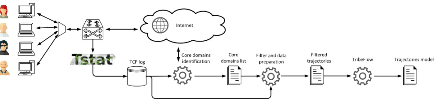
The workflow of our system is the one sketched in Figure 1. Users are connected to the Internet and we monitor the network at a point of presence where we collect and log information about each TCP connection (Section II). From this log, we extract all the domains, for each user. Next we design a methodology (Section III-A) that, thanks to some active measurements, get the subset of domains related to services intentionally visited by users. We (i) focus on those domains, and (ii) reconstruct meaningful trajectories over time (Section III-B). At this point, we learn the possibly best fitting TribeFlow model on such data (Section IV) and we analyze results (Section V).
To foster new studies and permit results reproducibil-ity, we contribute our dataset and model to the commu-nity. Anonymized trajectories of domains and their models are available to the public at http://bigdata.polito.it/content/ domains-web-users, while TribeFlow code is available at https://github.com/flaviovdf/tribeflow.
TCP log
Internet
Core domains list
Filtered
trajectories TribeFlow Trajectories model Users Terminals
Core domains identification
Filter and data preparation
Fig. 1. Workflow of the followed process.
II. DATASET
Our analysis relies on a dataset collected in our university campus. In the dataset, users’ terminals (usually PCs) are directly connected to the Internet via campus network (wired Ethernet) and uniquely identified by a statically assigned IP address, that is associated with one and only one user.
We rely on Tstat [8] to collect data. Tstat monitors each TCP connection, exposing information about more than 100 metrics, from IP addresses and port numbers, to fields coming from a DPI module. Here, we are interested in retrieving the domain name of the server being contacted. Tstat implements three techniques to get it. For HTTP flows, theHostheader is extracted from HTTP request. In case of TLS, the DPI module provides the Server Name Indication (SNI) field in Client Hello message. SNI is a TLS extension by which the client indicates the domain of the server that is trying to contact. At last, Tstat reports the domain name clients resolved via DNS queries prior to flows [5]. We combine these three sources to label each flow with the server name, giving higher priority to Host and SNI fields where more than one is present.
Our data contains traffic of approximately 2 500 terminals, collected at our university Campus in Torino during 4 weeks between January and February 2017. The dataset includes 691 millions flows and 404 k unique domains, corresponding to more than 136 k unique second level domains. No holidays or festivities occurred during this period. In total we monitored 113 TB of traffic, logging 229 GB of data.
Here, for each TCP connection we just consider: (i) the anonymized client IP address as terminal identifier, (ii) its department inside the Campus, (iii) the starting time and (iv) the end time of the connection, and (v) the server domain name.
A. Ethical and privacy risk mitigations
Both the data collection process and the collected data have been discussed, reviewed and approved by the ethical board of our University. We took all possible actions to protect leakages of private information from users. In particular, we anonymized the IP addresses of terminals using a technique based on irreversible hash function and only retained the data that is strictly needed for our study. We further anonymized
the server name in the datasets that we contribute to the community.
III. TRAJECTORIES EXTRACTION A. Identification of Core domains
When visiting a web-page, the browser application first downloads the main HTML document and then fetches all the objects of the page (images, scripts, advertisements, etc.). These are often hosted on external servers (e.g., CDNs) having different domains. We call Core domain a domain originally contacted to download the main HTML document of a page. Core domains are important since they are in-tentionally visited by users, likewww.facebook.com and en.wikipedia.org. We call Support domains those do-mains automatically contacted by visiting a Core domain, or by background applications, likestatic.10.fbcdn.net and dl-client.dropbox.com. Support domains do not contain useful information about user intention.
In the literature, previous works tackled the problem of identifying intentionally visited Core domains, also calleduser actions. Authors of [9] exploit the referer field in HTTP requests to reconstruct web-page structures from HTTP traces, while machine learning techniques are used by authors of [10] using the HTTP header. However, an important fraction of traffic is becoming encrypted, making the above approaches ineffective. Few efforts have been put in identifying user actions from encrypted traffic [11], [12]. These works aim at identifying user actions from flow level measurements examining traffic at runtime. Here, we aim at building a list of domains that typically contain user actions since they host actual web services.
We build on our previous work [13]. Given a domain, we visit the home-page it hosts. Based on the response, we classify it as a Core or Support domain. This is a classification problem, that we solve with a machine learning approach using a decision tree classifier. We consider an extensive list of features guided by domain knowledge, and let the classifier choose the ones that better allow it to separate Core and Support domains. Features include the length and the content type of the main HTML document (if present); the number of objects of the page and domains contacted by the browser to
fetch all objects; HTTP response code (e.g., 2xx, 3xx and 4xx); and whether the browser has been redirected to an external domain. We use active crawling, and visit the home page of each domain by means of Selenium automatic browser to extract page features.1
We build a labeled dataset that we use for training and test-ing, considering a list of 500 Core and 500 Support domains. More in detail, we picked the list of domains found in the Campus trace, sorted by number of visits. Then, we manually visited each home page corresponding to the domain name. We manually label such domain as a Core or a Support domain by looking at the rendered web page. We stop the labeling process when we reach 500 items for each class. We obtain a balanced labeled dataset that we make publicly available.2 For the decision tree, we opt for the J48 implementation of the C4.5 algorithm offered by Weka.3
Interestingly, the final decision tree results in a simple, efficient, and descriptive model which reads as: a) the main HTML document size must be bigger than 3357B and b) the browser must not be redirected to an external domain. Intuitively, support domains typically lack of real home page. When directly contacted, the server reply with short error messages. In some cases, Support domains redirect visitors to the service home page (e.g., fbcdn.net redirects on www.facebook.com). Despite its simplicity, overall accu-racy is higher than 96% when tested against 1 000 labeled domains, using 10–fold cross validations.
B. User trajectories reconstruction and characterization First, we characterize the trajectories in our dataset. These results will support the credibility of trajectories and therefore the model assumptions, as we will describe in Section IV.
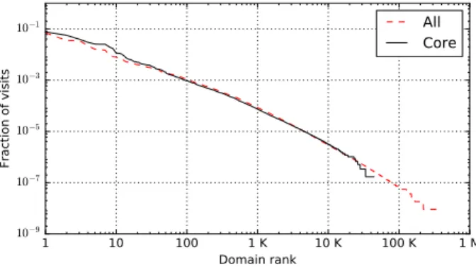
Applying the classifier to our dataset, we get that among the 404K domains, only 44K results Core. Figure 2 depicts two curves of domain popularity, where we rank each domain according to the fraction of visits directed towards it, for both all and Core domains. Notice the loglog scale. The pattern is similar for both the curves, even if the number of domain is quite different: a small portion of domains are popular and get the great majority of visits, with a long queue of domain getting few visits. Among the top 1 000 most popular domains (all), only 61 are Core domains. For Core domains, the popular domains are basically the ones with most page-views, according to Alexa4, i.e., Google, Facebook, Youtube, etc. These bring little information on the specific interests of a user. On the contrary, we expect the less popular domains to give specific information about user interests.
It is also interesting to analyse the connection length and inter-arrival time distributions. Both measures are important given that we want to reconstruct meaningful trajectories based on relative arrival time of the visit. Figure 3(a) reports the empirical Cumulative Distribution Function (CDF) of the
1http://www.seleniumhq.org/ 2http://bigdata.polito.it/content/domains-web-users 3http://www.cs.waikato.ac.nz/ml/weka/ 4https://www.alexa.com/topsites/countries/IT 1 10 100 1 K 10 K 100 K 1 M Domain rank 10−1 10−3 10−5 10−7 10−9 Fraction of visits
All
Core
Fig. 2. Popularity of domains, considering all of them or just Core ones.
connection duration. Core connections are in general longer. 80% of the connections last less than 3 minutes. The inter-arrival between two consecutive connections is shown in Figure 3(a). It is in general shorter than the duration of a connection. This means that is not uncommon to have multiple contemporary connections. This could imply that there are contemporary connections towards multiple sites and therefore could be complex to estimate the sequence of visits of the user. Moreover we see that many connections have a very small inter-arrival time (≤0.01s). This is due to the fact that browsers open multiple connections when visiting a web page. These connections could be towards many servers (Support domains), or even multiple connections towards the same domain.5 We analyze this aspect by showing the number of overlapping connections. Figure 3(b) shows the probability of number of overlapping connections. X axis is limited to 6 for ease of visualization. Analyzing all the domains, multiple contemporary connections are usual, and even tens of them are not rare. Even when limiting to Core domains, the probability of having no contemporary connections is only26%.
When building the user trajectory, multiple contemporary connections towards the same domain would artificially create sequences of visit to the same domain. To filter this artifact, we group together such overlapping trajectories towards the same Core domain. Specifically, we group visits to the same domain happening in the same time window of duration equal to the duration of the first connection. We then recompute the number of concurrent connections, showed by the curve labeled Core - filtered in Figure 3(b). Almost no connection is now contemporary to others (less than9%).
IV. MODELING USER TRAJECTORIES WITHTRIBEFLOW We want to model user habits focusing on how they move in the web from domain to domain. To achieve this goal, we rely on our recently proposed model called TribeFlow [6]. Here we provide a brief and simplified description of the methodology and invite to refer to [6] for all details.
Let us represent the trajectory of each user u ∈ U as a sequence of requests to domains. U is the set of users in the
0.01 s 0.1 s 1 s 10 s 1 min 5 min 1 h Time 0.0 0.2 0.4 0.6 0.8 1.0
CDF visits
Duration - All
Duration - Core
Intertime - All
Intertime - Core
(a) Duration and inter-arrival of connections
0 1 2 3 4 5 6 # contemporary visits 0.0 0.2 0.4 0.6 0.8 1.0 Frequency of visits
All
Core
Core - filtered
(b) Number of contemporary visits Fig. 3. Characterization of connections.
whole trace V. Similarly, d ∈ D represents a domain. We generalize the dataset V from a single edge network as a set of visits v ∈ V, with each visit being represented as a triple:
v= (u, t, d).trepresents a timestamp of the visit.
It is expected that real user behavior will be (i) non-stationary, and (ii) time heterogeneous [14]. In other words, user behavior change and evolve over time, and is different for each user. TribeFlow was designed to cope with the complex challenges of learning personalized predictive models of non-stationary, time heterogeneous, and transient (Markovian) user trajectories.
Let a trajectory from a users be comprised of the visits ordered by time. That is, the trajectory for user uis:Vu=<
(u, t0, d0),(u, t1, d1),· · ·,(u, tn, dn) >. TribeFlow objective is to capture the overall set of trajectories as a set of k transitions matrices of size|D|by|D|. Each matrix represents a stationary and time homogeneous first order Markov chain and characterize a latent environment z. Therefore, each environment is associated with the first order Markov chain P(di+1 | di, z). The domain di is associated with time ti, whereas di+1 is the next immediate visit at time ti+1. This chain captures the probability of going todi+1 given that the last visit was to domaindi, within environmentz. The number of environmentskcan be automatically inferred from the data with different methods [7].
For each user u, let us define a probability of interest, or strength, that this user has in environmentz,P(z|u). That is,
when a user is browsing the web, she selects a random environ-ment associated to her interests or needs (e.g., search engines, social networks, or e-commerce websites). This choice is done according toP(z|u). After selecting an environment, the user selects a domain based onP(di+1|di, z).
Based on the definitions above, the whole dataset of trajecto-ries are captured as random walks over random environments. Each environment captures a latent factor that leads to a user visiting a domain.
Given that for each user the overall behavior is captured as mixture (based on P(z | u)) of stationary and time homogeneous matrices (P(di+1|di, z)), the overall behavior captures a non-stationary, time heterogeneous, and transient system. Finally, TribeFlow can non-parametrically incorporate the inter-arrival time to model P(τ |z), with τ =ti+1−ti. The overall probability of a user transitioning between two domains within an environment is defined as:
P(di+1|di, u, z, τ, α, β, λ)
=P(di+1|z, β)P(di|z, β)P(τ|z, λ)P(z|u)
1−P(di|di, z, β)
α, β, andλare hyper parameters which are fixed to sensible defaults [6]. The goal of the model is to learn the matrices Θ (with k rows and |U | columns) and Φ (with |D| rows and k columns) that correspond to probabilities P(z | u)
and P(d | z), respectively6. After the model is trained, the probability P(di+1 | di, z) is simply defined as: P(di+1 | di, z) = P(di+1 | z)P(di | z) The probability matrix for each environment, as well as the strength of each user in an environment is learned through Gibbs Sampling (see [6] for details).
Learning the model on our dataset:using TribeFlow, we are able to summarize our large dataset of trajectories in a succinct and interpretable manner. For training the model, the only parameter we have to tune is the number of environments k. More environments allows to better approximate the trace, but increase the complexity of the models. We therefore use a weighted version of the error, obtaining a best number of environmentk= 30.
We train different models, each with 30 environments, by using: 1) the whole Campus trace, 2) the single Architecture department trace and 3) the Electronic department trace.
V. RESULTS
In this section, we analyze the model we created in Sec-tion IV and we show how it can be useful for studying the behaviour of the users.
A. Environments as clusters of common domains
Once we build the 30 environments, we manually inspect and analyse the most relevant domains inside them. We expect each domain dto be present in all the environments z, with a probability P(d|z). We can therefore sort the domains d
(a) Electronic dept. with many computer-science related domains
(b) Electronic dept. environment with many e-commerce domains
(c) Architecture dept. environment with many travel related domains
(d) Architecture dept. environment with many fashion related domains Fig. 4. Examples of top-10 domains in different environments of Electronic and Architecture departments, showed as word-clouds.
20000 40000 60000 80000 100000 Popularity 100 150 200 250 300 350 400 450 KL divergence 0 1 2 3 4 5 6 7 8 9 10 11 12 13 14 15 16 17 18 19 20 21 22 2324 25 26 27 28 29
(a) Campus dataset
250 500 750 1000 1250 Popularity 160 180 200 220 240 260 280 300 KL divergence 0 1 2 3 4 5 6 7 8 9 10 11 12 13 14 15 16 17 18 19 20 21 22 23 24 25 26 27 28 29
(b) Electronic department dataset
200 400 600 800 1000 1200 Popularity 100 125 150 175 200 225 250 275 KL divergence 0 1 2 3 4 5 6 7 8 910 1112 13 14 15 16 17 18 1920 21 22 23 24 25 26 27 28 29
(c) Architecture department dataset Fig. 5. Diversity and popularity of the environments for different datasets.
accordingly to the probability distribution Φz(d) = P(d|z) inside each environment, and then visually inspect the most probable domains. By construction, we expect to have domains that are usually sequential in time within the same environ-ment. Results show that most of the environments contains the most popular and generic domains, e.g., search engines and social networks. However, we clearly see some specific domains to dominate in some environments, i.e., the model let domains with the same topic to emerge in some specific environment only. For instance, we observe news, weather forecast, engineering forums and science journals related web-site to dominate different environments. This reflects the user habits of browsing asequenceof domains with the same topic. To illustrate this, consider the models extracted from users within the Electronic and Architecture departments. Figure 4 illustrates the word-clouds of the top 10 domains of specific environments7. Observe how expressive are the word-cloud in describing the topic of each environment.
B. Analysis of diversity and popularity of environments To quantify how the 30 environments are different among each other, we use as metric the Kullback-Leibler (KL) diver-gence [15]. KL diverdiver-genceDKL(Φz1kΦz2)measures how one
probability distributionΦz1 diverges from a second, expected
probability distribution Φz2. It is defined as:
7We removed common domains, i.e., Google, Facebook, and Youtube
because they are among the most popular in all the environments.
DKL(Φz1kΦz2) = X d∈D Φz1(d) log Φz1(d) Φz2(d)
In our case, the expectation is taken using the probabilities of each domain d ∈ D. Φz1 and Φz2 are the domain
probabilities for environments z1 andz2 (Φz1(d) =P(d|z1)
and Φz2(d) = P(d|z2)). Therefore, environments z quite
different from all the others will have a large value of DKL(z) = PziDKL(ΦzkΦzi), that we call KL divergence
for environment z.
We further compute the mean expected number of visits for each environment, namely thepopularityof the environments z, computed asV(d)·P(d|z), whereV(d)is the number of visits towards domaindin the original dataset.
We plotDKL(z)versusV(d)·P(d|z)for eachz. Figure 5 shows results for: (a) the whole Campus, (b) Electronic, and (c) Architecture departments. Each environment is labeled with a different number for ease of visualization. We see in all cases a clear trend: the most popular environments are also the one that are less diverse from each other. These environments are generic, and thus less interesting to inspect. On the other hand, environments with large KL divergence usually have a low number of expected visits. These environments are the most peculiar ones. For example, consider environment 2 in Campus traces. Analyzing its most popular domains, it appears related to users/devices that often go to visit sony.com and sony.it, possibly because they hosts home-pages automatically visited by software installed on those users’ devices. Other
To environment From environment 102 101 100 (a) Campus To environment From environment 102 101 100 (b) Electronic To environment From environment 102 101 100 (c) Architecture Fig. 6. Transition probability heat-maps among the environments.
examples of peculiar environments include domains related to torrents and movie streaming portals, and to popular bank ac-counts. This method of analysis offers the analyst an automatic way to highlight interesting environments.
C. Transitions in communities
In the previous subsections we showed how interests are different in communities of people. We now show how com-munities switch among environments. In Figure 6 we show the heat-maps of the transition probability matrix P(z1|z2) from environmentz1to another environmentz2, in logarithmic scale. This matrix can be easily computed from the model parameters. By construction, elements of a row has to sum to 1, while the sum on the element of a column represents the probability of landing to that particular environment. We sort the columns by such (reversed) sum of probabilities. We see how for Campus datasets, transitions are usually towards a single popular environment that contains generic websites (on the foremost left in Figure 6(a)). On the other hand, transitions on Architecture and Electronic departments are spread towards many topics, some of which are specific of each department. Among all the possible 870 transitions, only 86 for the Campus are above the random probability, while this number increases to 129 for Electronic and 146 for Architecture department. This means that inside the departments people are much more homogeneous and tends to visit more evenly the peculiar environments. Even if very different between each others, these environments are in general more common within the same community of people.
VI. CONCLUSIONS AND FUTURE WORK
In this work, we described how to create from passive traces meaningful trajectories of users on the web, and then how to represent them in a succinct and interpretable manner. We showed that our model allows to automatically and easily in-spect the interests of users and communities, and to highlights transitions and diversity is such clusters of domains. We plan to extend our work in order to: (i) study temporal evolution of trajectories and environments, (ii) apply our methodology to much bigger datasets coming from ISPs, and (iii) propose personalized recommendation systems for users browsing.
REFERENCES
[1] N. Kammenhuber, J. Luxenburger, A. Feldmann, and G. Weikum, “Web search clickstreams,” inProceedings of the 6th ACM SIGCOMM Conference on Internet Measurement.
[2] I. Mele, “Web usage mining for enhancing search-result delivery and helping users to find interesting web content,” in Proceedings of the Sixth ACM International Conference on Web Search and Data Mining. [3] T. Joachims, “Optimizing search engines using clickthrough data,” in Proceedings of the Eighth ACM SIGKDD International Conference on Knowledge Discovery and Data Mining, July 23-26, 2002, Edmonton, Alberta, Canada, 2002, pp. 133–142.
[4] G. Wang, T. Konolige, C. Wilson, X. Wang, H. Zheng, and B. Y. Zhao, “You are how you click: Clickstream analysis for sybil detection,” in Proceedings of the 22Nd USENIX Conference on Security.
[5] I. N. Bermudez, M. Mellia, M. M. Munafo, R. Keralapura, and A. Nucci, “Dns to the rescue: Discerning content and services in a tangled web,” inProceedings of the 2012 Internet Measurement Conference. [6] F. Figueiredo, B. Ribeiro, J. M. Almeida, and C. Faloutsos, “Tribeflow:
Mining and predicting user trajectories,” in Proceedings of the 25th International Conference on World Wide Web.
[7] F. Figueiredo, B. Ribeiro, J. M. Almeida, N. Andrade, and C. Faloutsos, “Mining online music listening trajectories,” inInternational Society for Music Information Retrieval Conference, 2016.
[8] M. Trevisan, A. Finamore, M. Mellia, M. Munafo, and D. Rossi, “Traffic analysis with off-the-shelf hardware: Challenges and lessons learned,” IEEE Communications Magazine, vol. 55, no. 3, pp. 163–169, 2017. [9] G. Xie, M. Iliofotou, T. Karagiannis, M. Faloutsos, and Y. Jin, “Resurf:
Reconstructing web-surfing activity from network traffic,” inIFIP Net-working Conference, 2013, Brooklyn, New York, USA, 22-24 May, 2013, 2013, pp. 1–9.
[10] L. Vassio, I. Drago, and M. Mellia, “Detecting user actions from HTTP traces: Toward an automatic approach,” in2016 International Wireless Communications and Mobile Computing Conference (IWCMC), Paphos, Cyprus, September 5-9, 2016, 2016, pp. 50–55.
[11] M. Conti, L. V. Mancini, R. Spolaor, and N. V. Verde, “Analyzing android encrypted network traffic to identify user actions,”IEEE Trans-actions on Information Forensics and Security, vol. 11, no. 1, pp. 114– 125, 2016.
[12] B. Saltaformaggio, H. Choi, K. Johnson, Y. Kwon, Q. Zhang, X. Zhang, D. Xu, and J. Qian, “Eavesdropping on fine-grained user activities within smartphone apps over encrypted network traffic,” inProceedings of the WOOT16. ACM, 2016, pp. 59–78.
[13] L. Vassio, D. Giordano, M. Trevisan, M. Mellia, and A. P. C. da Silva, “Users’ fingerprinting techniques from tcp traffic,” inProceedings of the Workshop on Big Data Analytics and Machine Learning for Data Communication Networks.
[14] M. Aly, S. Pandey, V. Josifovski, and K. Punera, “Towards a robust modeling of temporal interest change patterns for behavioral targeting,” in Proceedings of the 22Nd International Conference on World Wide Web, ser. WWW ’13. New York, NY, USA: ACM, 2013, pp. 71–82. [15] S. Kullback and R. A. Leibler, “On information and sufficiency,”Ann. Math. Statist., vol. 22, no. 1, pp. 79–86, 1951.