Bivariate Gaussian random fields : models, simulation, and inference

(1)

Bivariate Gaussian random fields:

models, simulation, and inference

Inauguraldissertation zur Erlangung des akademischen Grades eines

Doktors der Naturwissenschaften der Universit¨

at Mannheim

vorgelegt von

Olga Moreva

aus Moskau, Russland

(2)

Dekan: Dr. Bernd L¨ubcke, Universit¨at Mannheim

Referent: Prof. Dr. Martin Schlather, Universit¨at Mannheim

Korreferent: Prof. Dr. Tilmann Gneiting, Karlsruher Institut für Technologie Tag der mündlichen Prüfung: 22. Juni 2018

(3)

Abstract

Spatial data with several components, such as observations of air temperature and pressure in a certain geographical region or the content of two metals in a geological deposit, require models which can capture the spatial dependence structure of individual components and the relationship between them. In a wealth of applications, multivariate Gaussian random fields are sensible models for multivariate spatial data and their second order structure specifies the marginal correlations and the cross-correlations between the components. In this thesis we focus on covariance models and simulation techniques for bivariate fields.

In Chapter 2 we summarize some definitions and facts from univariate and multivariate Geostatistics which are essential for the subsequent chapters.

Chapter 3 introduces two novel bivariate parametric covariance models, the powered ex-ponential (or stable) covariance model and the generalized Cauchy covariance model. Both models allow for flexible smoothness, variance, scale, and cross-correlation parameters. The smoothness parameter is in (0,1]. Additionally, the bivariate generalized Cauchy model allows for distinct long range parameters. The results are based on general sufficient conditions for the positive definiteness of 2×2-matrix valued functions. These conditions are easy to check, since they require only computing the derivatives of a bivariate covariance function and calculating an infimum of a function of one variable. We also show that the univariate spherical model can be generalized to the bivariate case with spherical marginal and cross-covariance functions only in a trivial way.

Circulant embedding is a powerful algorithm for fast simulation of stationary Gaussian ran-dom fields on a rectangular grid in Rn, which works perfectly for compactly supported

co-variance functions. Cut-off circulant embedding techniques have been developed for univariate random fields for dimensions up to R3 and rely on the modification of a covariance function

outside the simulation window, such that the modified covariance function is compactly sup-ported. In Chapter 4 we propose extensions of the cut-off approach for bivariate Gaussian random fields. In particular, we provide a method for simulating bivariate fields with a bi-variate powered exponential covariance model and the full bibi-variate Mat´ern covariance model for certain sets of parameters. On the way we extend the cut-off circulant embedding method even for univariate models.

In Chapter 5 we illustrate the use of the bivariate powered exponential model for a data example.

(4)

(5)

Zusammenfassung

Räumliche Daten mit mehreren Komponenten, wie Beobachtungen von Lufttemperatur und Atmosphärendruck in einer bestimmten geographischen Region oder der Gehalt von zwei Met-allen in einer geologischen Lagerstätte, erfordern Modelle, die die räumliche Abh¨ angigkeitsstruk-tur einzelner Komponenten und die Beziehungen zwischen ihnen erfassen. In einer Vielzahl von Anwendungen sind multivariate Gauß’sche Zufallsfelder sinnvolle Modelle für multivariate räumliche Daten und ihre Struktur zweiter Ordnung spezifiziert die marginalen Korrelationen und die Kreuzkorrelationen zwischen den Komponenten. Diese Arbeit konzentriert sich auf Kovarianzmodelle und Simulationstechniken für bivariate Felder.

Kapitel 2 fasst einige Definitionen und Fakten der univariaten und der multivariaten Geo-statistik zusammen, die grundlegend f¨ur die folgenden Kapitel sind.

Kapitel 3 stellt zwei neuartige bivariate parametrische Kovarianzmodelle vor, das potenzex-ponentielle (oder stabile) Kovarianzmodell und das verallgemeinerte Cauchy-Kovarianzmodell. Beide Modelle ermöglichen flexible Glättungs-, Varianz-, Skalierungs- und Kreuzkorrelationspa-rameter. Der Glättungsparameter ist in (0,1]. Zusätzlich erlaubt das bivariate verallgemeinerte Cauchy-Modell verschiedene Langzeitparameter. Die Ergebnisse basieren auf hinreichenden Bedingungen für die positiv Definitheit von 2×2-Matrix-wertigen Funktionen. Diese Bedin-gungen sind einfach zu überprüfen, da nur die Ableitungen einer bivariaten Kovarianzfunktion berechnet werden müssen, und das Infimum einer Funktion von einer Variablen zu bestimmen ist. Zudem wird gezeigt, dass das univariate sphärische Modell nur auf triviale Weise auf den bivariaten Fall mit sphärischen marginalen und Kreuzkovarianzfunktionen verallgemeinert werden kann.

Circulant Embedding ist ein leistungsfähiger Algorithmus zur schnellen Simulation von sta-tionären Gauß’schen Zufallsfeldern auf einem rechteckigen Gitter inRn, der perfekt für

Kovar-ianzfunktionen mit kompaktem Träger funktioniert. Cut-off circulant Embedding Techniken wurden für univariate Zufallsfelder für Dimensionen bis zu R3 entwickelt und basieren auf

der Modifikation einer Kovarianzfunktion außerhalb des Simulationsfensters, sodass die mod-ifizierte Kovarianzfunktion einen kompakten Träger hat. In Kapitel 4 werden Erweiterungen des Cut-off-Ansatzes für bivariate Gauß’sche Zufallsfelder vorgeschlagt. Insbesondere wird eine Methode zur Simulation von bivariaten Feldern mit einem bivariaten exponentiellen Kovarianz-modell und dem vollständigen bivariaten Matérn-Kovarianzmodell für bestimmte Parameter-sätze bereitgestellt. Dabei wird die Cut-off circulant Embedding-Methode auch für univariate Modelle erweitert.

Kapitel 5 illustriert die Verwendung des bivariaten potenzexponentiellen Modells anhand eines Datenbeispiels.

(6)

(7)

Acknowledgements

I am indebted to my advisor Prof. Dr. Martin Schlather, whose solid support and guidance made my thesis work possible. I owe a lot of gratitude to him for always being there for me and I really appreciate his willingness to meet me at short notice even in busy times. His ability to explain difficult things clearly helped me many times to establish the direction of my research. I would like to thank Prof. Dr. Tilmann Gneiting for being a great second dissertation advisor. I am especially grateful for his valuable and extremely prompt feedback on my papers. Workshops in HITS organized by Prof. Dr. Tilmann Gneiting broadened my mathematical horizon and provided inspiration for my research. I also thank Prof. Dr. Sebastian Engelke for orginizing my stay at École Polytechnique Fédérale de Lausanne in the end of 2016.

I am grateful to all my colleagues for many interesting discussions during seminars and workshops at the RTG 1953. My special thank goes to Elias Stehle, Alexander Kalinin and Artem Makarov for their help during my first months in Mannheim. I would like to express my sincere gratitude to Dr. Kirstin Strokorb, Dr. Eva L¨ubcke and Stefan Schnabel for their extensive support. Many thanks to Lena Reichmann for cheerful conversations and pleasant lunch times. I am immensely grateful to Dr. Martin Dirrler for the attentive proofreading of my thesis, his useful comments, and the constant encouragement.

Financial support by the Deutsche Forschungsgemeinschaft (DFG) through the Research Training Group RTG 1953 ’Statistical Modeling of Complex Systems and Processes’ and by Mannheim University through the dissertation completion grant is also gratefully acknowl-edged.

Finally, I have no words to express my gratitude to my family and my boyfriend Nikolaj for their continuous support, unconditional love and unshakable faith in me.

(8)

(9)

1 Introduction

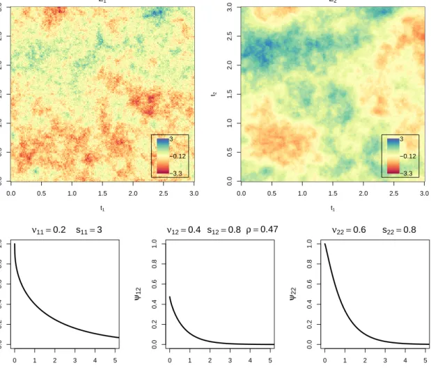
Multivariate data measured in space arise in a variety of disciplines including soil science (Lark and Papritz, 2003), ecology (Pelletier et al., 2009), mining (Zawadzki et al., 2013), geology (Mery et al., 2017) and meteorology (Hewer et al., 2017). Air temperature and pressure in a certain geographical region or the content of two metals in a geological deposit are the examples of spatial processes with two components. Spatial dependence within and between the components is exploited in particular when the component of interest is not exhaustively sampled, whereas the measurement of other components can be easily carried out, e.g. in soil sciences (Goovaerts (1999) and Atkinson et al. (1992)). An appropriate multivariate spatial covariance model gives more sensible results for spatial interpolation than univariate models, see for example Cressie and Zammit-Mangion (2016). In environmental and climate sciences it is important to model spatial meteorological data jointly in order to reflect spatial dependence within and between components adequately (see the discussions in Feldmann et al. (2015), Berrocal et al. (2007), and Gel et al. (2004)); otherwise the obtained results might be unsound. Multivariate Gaussian random fields, characterized by their mean and covariance functions, are the basis for modeling spatial data in these areas. Classical textbooks on univariate and multivariate geostatistics include Cressie (1993), Chil`es and Delfiner (1999), Lantuejoul (2001), Wackernagel (2003), and Goovaerts and Goovaerts (1997). For simplicity, in the theoretical part of the thesis we consider zero mean random fields. Then a covariance function describes the properties of the corresponding Gaussian random field. Consider, for example, a realization of a Gaussian random field with two components shown in two upper plots in Figure 1.1. This field has the bivariate Mat´ern covariance model (Gneiting et al., 2010), which is plotted under the realizations. The functions ψ11 and ψ22, called marginal covariances, describe the

properties of the first and the second field respectively. The behavior of the covariance function at the origin largely reflects the smoothness of the corresponding field (Gneiting, 2002). In the bivariate Mat´ern model the smoothness of each field is controlled by the corresponding parameterνii>0, i= 1,2. In Figure 1.1, ν22> ν11 and therefore the realization on the right

hand side is smoother than the one on the left hand sight. The scale parametersii>0,i= 1,2, controls the decay of the marginal correlation with the distance. For example, the correlation of any two observations of the first field for the larger distance is higher than the correlation of any two observations of the second field, therefore the upper left plot is more colorful than the upper right one. The middle picture in the lower panel of Figure 1.1 is the graph of the cross-covariance functionψ12, which describes the covariance structure between the two components.

The scale parameter s12 controls the correlation decay between the components. Thus, the

correlation between the observation of the first field and the observation of the second field is maximum at zero distance and it decreases as the distance increases. While the maximum of a marginal covariance function is always at the origin, the maximum of the cross-covariance function (assuming positive correlation between a given variable pair) may be shifted away from the origin, which is typical when one component affects another component with some delay (Wackernagel (2003), Hansen (2018)). However, we focus on covariance functions which

(12)

4 Chapter 1. Introduction 0 1 2 3 4 5 0.0 0.2 0.4 0.6 0.8 1.0 r ψ11 ν11=0.2 s11=3 0 1 2 3 4 5 0.0 0.2 0.4 0.6 0.8 1.0 r ψ12 ν12=0.4 s12=0.8 ρ =0.47 0 1 2 3 4 5 0.0 0.2 0.4 0.6 0.8 1.0 r ψ22 ν22=0.6 s22=0.8 0.0 0.5 1.0 1.5 2.0 2.5 3.0 0.0 0.5 1.0 1.5 2.0 2.5 3.0 Z1 t1 t2 3 −0.12 −3.3 0.0 0.5 1.0 1.5 2.0 2.5 3.0 0.0 0.5 1.0 1.5 2.0 2.5 3.0 Z2 t1 t2 3 −0.12 −3.3

Figure 1.1: A realization of a bivariate Gaussian random field (upper two plots) with the bivariate Mat´ern covariance model (lower three plots). The stationary and isotropic covariance function depends on the distance r between the locations. The lower left and the right plots show the marginal covariance functionsψ11 andψ22, respectively.

depend only on the distance between observations, i.e. they are invariant with respect to the location of observations and the direction of the separation vector.

A covariance function must guarantee that the variance of an arbitrary linear combination of observations of any involved components, taken at arbitrary spatial locations is nonnegative. In this thesis we concentrate on constructing matrix-valued functions that satisfy this require-ment, on simulation techniques which are suitable for these functions and on inference with them. In Chapter 2 we summarize some definitions and facts from univariate and multivariate Geostatistics which are crucial for the subsequent chapters.

A comprehensive overview of recent covariance functions for multivariate geostatistics is found in Genton and Kleiber (2015) and Schlather et al. (2015). Among these models is the linear model of coregionalization (LMC), see Goulard and Voltz (1992) and Wackernagel (2003). Although it is widely used by practitioners, it lacks flexibility, since all direct and cross variograms share the same set of basic structures. This means, in particularly, that the

(13)

5

smoothness of any component is equal to the smoothness of the roughest latent process, and, thus, the standard approach LMC does not admit individually distinct smoothness properties, unless structural zeros are imposed on the latent process coefficients (Gneiting et al. (2010) and Goovaerts and Goovaerts (1997)). Models with compact support are introduced in Du and Ma (2013), Porcu et al. (2013), Daley et al. (2015) and Schlather et al. (2017). Kleiber (2017) studies the properties of multivariate random fields in the frequency domain. Cressie and Zammit-Mangion (2016) develop a conditional approach for constructing multivariate models. Genton and Kleiber (2015) pose the question how to characterize a parameter set of the valid multivariate powered exponential (or stable) model. In Chapter 3 we give a partial answer to this question, providing sufficient conditions for the positive definiteness of a bivariate model. In a similar way we can also formulate sufficient conditions for the positive definiteness of the bivariate generalized Cauchy model. These models are flexible, intuitive and easily interpretable: in both models three parameters characterize the smoothness of the covariances of process components and the cross-covariance. Further three parameters model the long-range behaviour in the bivariate Cauchy model. The smoothness parameters of marginal covariances in both models are restricted to values in (0,1]. The results are based on general sufficient conditions for the positive definiteness of a 2×2-matrix valued functions. These conditions require only computing the derivatives of a bivariate covariance function of order two and three inRand inR3, respectively, and calculating an infimum of a function of one variable. We also

show that the univariate spherical model can be generalized to the bivariate case with spherical marginal and cross-covariance functions only in a trivial way. We collect some new bivariate models, whose construction follows directly from Schoenberg’s theorem.

Development of many multivariate covariance models led to the increasing interest in sim-ulation algorithms. Cholesky decomposition is not suitable for samples with a larger number of locations, not least because the computing time of the algorithm is cubic in the number of variables. For functions possessing spectral densities with closed formulae, the spectral turn-ing bands algorithm can be used (Arroyo and Emery (2017) and Emery et al. (2016)). The multivariate turning bands method is implemented in the R packageRandomFields(Schlather et al., 2017). Both turning bands methods are faster than the Cholesky decomposition and can be performed for any configuration of the target locations, but they produce realizations that are only approximately Gaussian. Under certain conditions on a covariance function the multi-variate version of the circulant embedding algorithm, presented in Chan and Wood (1999) and explained in detail in Helgason et al. (2011), produces Gaussian realizations. However, simi-larly to the univariate case, for many multivariate covariance models that do not have compact support exact simulation is not possible. Cut-off circulant embedding techniques have been developed for univariate random fields for dimensions up to R3 and rely on the modification

of a covariance function outside the simulation window, such that the modified covariance function is compactly supported. In Chapter 4 we propose extensions of the cut-off approach for univariate and bivariate Gaussian random fields. In particular, we provide a method for simulating bivariate fields with a bivariate powered exponential covariance model and the full bivariate Mat´ern covariance model for certain sets of parameters on a grid.

In Chapter 5 we illustrate the use of the bivariate exponential model for a data example on the content of copper and zinc in the top soil of a 14 km2 region in Swiss Jura. We compare the performance of bivariate powered exponential model to the traditional linear model of coregionalization and the bivariate Mat´ern model.

(14)

(15)

2 Preliminaries

We briefly summarize some basic definitions and facts about covariance functions and var-iograms of univariate and multivariate Gaussian random fields, which are necessary in the subsequent parts.

There is sometimes a confusion between the notions multidimensional and multivariate in the literature. Hereinafter we call a random field Z univariate if it has only one component, and multivariate if it has m ≥ 1 components, i.e. Z(x) = (Z1(x), . . . , Zm(x)), x ∈ Rn. In

Chapters 3 and 4 we will be concerned withbivariatefields, i.e.m= 2. The term multidimen-sional refers to the index set ofZ, i.e. to the dimension ofx. For example, a one dimensional univariate field is just a temporal stochastic process, a two dimensional univariate field is a ’classical’ random field and a three dimensional bivariate fieldZ(x) = (Z1(x), Z2(x)) has two

components withx∈_R3_.

The finite dimensional distributions of a multivariate Gaussian random fieldZ(x) are multi-variate normal and thus the distribution of the field is uniquely characterized by its mean and covariance function. For simplicity, we assume in the theoretical part of the thesis that the random field is centered, i.e.EZ(x) = 0 for allx∈Rn. We denote the covariance function by

C(x, y) = Cov(Z(x), Z(y)), x, y∈Rn. Clearly, a covariance function C of a multivariate field

is a matrix-valued function, whose diagonal elementsCii(x, y), i= 1, . . . , m, are the marginal covariance functions and the off-diagonal elementsCij(x, y) are the cross-covariance functions of the components of the process 1≤i6=j ≤m. The content of the next two sections is based mostly on Wackernagel (2003), Chil`es and Delfiner (1999) and Yaglom (1987).

2.1 Multivariate covariance functions

A covariance functionC is calledstationary if for any x, h∈Rn andi, j = 1, . . . , mit holds:

Cij(x+h, x) =Cij(h,0) =:Cij(h).

A stationary multivariate covariance function is not necessarily an even or odd function. In general, we have

Cij(−h)6=Cij(h), but

Cij(h) =Cji(−h).

Cisstationary and isotropicif additionallyC(h1) =C(h2) wheneverkh1k=kh2k, i.e. marginal

covariance functions and cross-covariance functions depend only on the distance between the variables locations. Hereinafter we write C(r) instead of C(h) with r =khk, whenever C is stationary and isotropic.

We denote by Φn the set of continuous functionsϕ: [0,∞)7→Rsuch that the map (x, y)7→

ϕ(||x−y||) is positive definite on Rn. Analogously, Φmn denotes the class of mappings ϕ = [ϕij(·)]m_i,j₌₁ : [0,∞)7→Rm×m with eachϕij being continuous, such that

C(x, y) = [ϕij(||x−y||)]m_i,j₌₁, x, y∈Rn,

(16)

8 Chapter 2. Preliminaries

is anm×m matrix-valued covariance function onRn.

We recall that a covariance function must be positive definite, i.e. it guarantees that the variance of an arbitrary linear combination of observations of any involved componentsZi(x),

i= 1, . . . , m, taken at arbitrary spatial locations is nonnegative. That is, C is symmetric and for any p∈_N, a1, . . . , ap ∈Rm,and x1, . . . , xp ∈Rn it must hold

p X

i=1

aT_i C(xi−xj)aj ≥0.

Reversely, for each positive definite function C there exists a Gaussian random field with C

being its covariance function. Thus, the terms covariance function and positive definite function are interchangeable.

Example 2.1 (Linear model of coregionalization, Goulard and Voltz (1992); Wackernagel (2003))

The basic statement of the linear model of coregionalization (LMC) is that each variable Zi,

i = 1, . . . , m, of a multivariate field Z is a linear combination of p independent univariate stationary random fields with unit variance {Yk, k= 1, . . . , p}.

Zi(x) = p X

k=1

aikYk(x), x∈Rn.

The resulting multivariate covariance is

Cij(h) = p X

k=1

aikajkρk(h), h∈Rn,

where ρk(h) is a correlation function of Yk and A = [aik]m,pi,k=1 is a m×p full rank matrix.

Although this model is widely used among practitioners, it lacks flexibility and its limitations are discussed in Gneiting et al. (2010)

Example 2.2 (Convolution)

Suppose that c1, . . . , cm are real-valued functions on Rn which are both integrable and

square-integrable. The matrix-valued function defined by equation

Cij(h) = (ci∗cj)(h), h∈Rn, i, j = 1, . . . , m,

where the asterisk∗denotes the convolution operator, is a matrix-valued covariance function on

Rn (Theorem 2 in Gneiting et al. (2010)). These models are introduced in Ver Hoef and Barry

(1998) and Gaspari and Cohn (1999); the multivariate parsimonious Mat´ern covariance model (Gneiting et al., 2010) serves as an example of this construction. Kleiber (2017) discusses the properties and limitations of this class of models.

For a better understanding of the properties of a covariance function it is often useful to examine its Fourier transform. A stationary covariance functionC has the following spectral representation

C(h) = Z

Rn

(17)

2.1. Multivariate covariance functions 9

where the increments ∆F(x) = F(x+ ∆x) −F(x) of the matrix-valued function F(x) are positive semidefinite matrices for all x ∈ Rn and ∆x ≥ 0 (componentweise). The diagonal

elements Fii(x), i = 1, . . . , m, are real, non-decreasing and bounded; the off-diagonal terms

Fij(x), i6=j, i, j= 1, . . . , m,are in general complex-valued and of finite variation. Conversely, any matrix of continuous functionsC(h) is a matrix-valued covariance function, if the matrices of increments ∆F(x) are positive semi-definite for any x ∈ _Rn _{and ∆}_x _≥ _{0. This result} is a multidimensional generalization of Cramer’s theorem (Cramer, 1940), which is itself a multivariate generalization of Bochner’s theorem (Bochner, 1955) and can be found in Gikhman and Skorokhod (2004), Yaglom (1987), and Wackernagel (2003).

When the Cij are additionally absolutely integrable, there exists a spectral density matrix such that

C(h) = Z

Rn

eihh,xif(x)dx for all h∈_Rn

andf(x) is a positive semi-definite matrix for all x∈_Rn_{, see Yaglom (1987).}

IfC is stationary and isotropic, the Fourier transform in (2.1) can be replaced by a Hankel transform, that is,

C(r) = 2(n−2)/2Γn 2

Z ∞

0

(ru)−(n−2)/2J₍_n−2)/2(ru)dG(u), r ≥0, (2.2)

whereGij are the functions of bounded variation having the property that the matrix ∆G(u) =

G(u+ ∆u)−G(u) is positive semidefinite for allu,∆u >0 (Yaglom, 1987). Analogous Hankel transform for the spectral density reads

C(r) = (2π)n/2

Z ∞

0

(ru)−(n−2)/2J(n−2)/2(ru)un−1f(u)du, r≥0,

where [f(u)]m_i,j₌₁ is a positive semi-definite matrix for all u ≥0. This result is a nultivariate generalization of Schoenberg’s theorem (Schoenberg, 1938). The inversion formula for the spectral densityf, which exists if R∞

0 r n−1_|_C₍_r₎_|_{dr <}_∞_{, is} f(u) = (2π)−n/2 Z ∞ 0 (ur)−(n−2)/2J(n−2)/2(ur)rn−1C(r)dr,

see for example Stein (1999). In the subsequent Chapters 3, 4 and 5 we restrict our attention to stationary and isotropic bivariate covariance models, whose components stem from the same family, i.e. to models of the form

C(r) = σ₁2ψ11(r) ρσ1σ2ψ12(r) ρσ1σ2ψ12(r) σ22ψ22(r) , (2.3)

where σi > 0 is the variance of the field Zi, ψij(·) = ψ(·|θij, sij) is a continuous univariate stationary and isotropic correlation function, which depends on a scale (or range) parameter

sij >0, i, j = 1,2,and another optional parameterθij = (θij1, ..., θkij) withk∈N(e.g. smooth-ness, long range behaviour). Necessarily,|ρ| ≤ 1. Note that isotropy implies ψ12(r) =ψ21(r).

Furthermore, we choose σ1 = σ2 = 1, since the general case follows immediately from the

following fact: C(r) = σ1 0 0 σ2 × ψ11(r) ρψ12(r) ρψ12(r) ψ22(r) × σ1 0 0 σ2 .

(18)

10 Chapter 2. Preliminaries

For instance, the multivariate Mat´ern model (Gneiting et al., 2010; Apanasovich et al., 2012) is a representative of this class with

ψ(r|ν, s) = 2

1−ν Γ(ν)(sr)

ν_K ν(sr),

wheres >0 is a scale parameter,ν >0 is a smoothness parameter andKν is a modified Bessel function of the second kind. The bivariate powered exponential model (Moreva and Schlather, 2017) also belongs to the class (2.3) with

ψ(r|α, s) =e−(sr)α,

wheres >0 is a scale parameter and α∈(0,2] is a smoothness parameter.

The class given by (2.3) can be seen as a generalization of the class of separable models introduced by Mardia and Goodall (1993), where a multivariate covariance factorizes into a product of a covariance matrixR and a univariate correlation functionψ(·), i.e.

Cij(r) =Rijψ(r), r≥0, i, j= 1, . . . , m.

That is, a separable model assumes that all components share the same spatial correlation structure and differ only in their variances. In particular, the scale parameter is the same for both marginal and cross-covariances. The class (2.3) is more flexible allowing each field to have distinct smoothness, scale, and variance parameters and admitting flexible cross-correlation between the fields. Given a univariate correlation function ψ, our goal in Chapter 3 is to find the parameter sets for which the functionC in (2.3) is a valid covariance function. Clearly, if the components are uncorrelated, i.e.ρ = 0, thenC is always a bivariate covariance function. Thus, we are interested in the cases when|ρ|>0.

2.2 Variograms

In Section 4.3 we focus on intrinsically stationary univariate random fields. Intrinsic station-arity is a weaker assumption than stationstation-arity. A random fieldZ withE(Z(x)−Z(y))2 <∞,

x, y∈Rn is called intrinsically stationary ifE(Z(x+h)−Z(x)) andE(Z(x+h)−Z(x))2 do

not depend onx for all h∈_Rn_{. Then we define the}_variogram

γ(h) = 1

2E(Z(x+h)−Z(x))

2_.

We recall that a function γ :Rn 7→ R is negative definite, if for any p ∈ N, x1, . . . , xp ∈Rn,

anda1, . . . , ap ∈R, such thatPpi=1ai = 0, the following inequality holds

p X i=1 p X j=1 aiγ(xi−xj)aj ≤0.

Theorem 2.3 (Gneiting et al. (2001))

If γ is a real symmetric function in Rn satisfyingγ(0) = 0, the following properties are

equiv-alent.

(19)

2.2. Variograms 11

(ii) The function γ is negative definite.

(iii) For alla >0,exp(−aγ(·)) is a covariance function.

The equivalence of (i) and (ii) mimics the characterization of covariances as positive definite functions. Theorem 2.3 extends known result (see the references in Gneiting et al. (2001)) by removing the additional assumption of continuity ofγ.

A stationary random field is always intrinsically stationary, but the converse is not true: the Wiener process is a counterexample. A stationary field has a bounded variogram γ which is linked with the covariance functionC by the relation

γ(h) =C0−C(h), h∈Rn, (2.4)

whereC0 =C(0).If the variogramγ(h) of an intrinsically stationary random field is bounded,

there exists a constant C0 > 0 such that C(h) = C0 −γ(h) is a covariance function. The

minimal value of C0 is of great interest because higher variances can always be achieved by

adding a spatially constant, independent Gaussian random variable to a random field. Gneiting et al. (2001) give the minimal value of C0 for bounded variograms. If γ is unbounded, then

(2.4) can hold locally, i.e. for|h| ≤r and somer >0.The existence and minimum value of C0

in (2.4) is discussed in Gneiting et al. (2001).

Finally, the rate with which a variogram γ(h) of a centered field can increase to infinity is constrained by lim khk→∞ γ(h) khk2 = 0, h∈R n_.

(20)

(21)

3 Bivariate covariance models

We discuss a sufficient condition and a necessary condition for the positive definiteness of models from the class (2.3). We consider some examples of this class and introduce novel bivariate models, built on Schoenberg’s theorem and on the sufficient condition. This chapter is partially based on Moreva and Schlather (2017).

3.1 Models obtained by spectral approach

We collect some new examples of the class (2.3). The proof of positive definiteness (or the contrary) of these models is based on Schoenberg’s theorem. Hereinafter we denote by fij the spectral density of a correlation function ψij, i, j = 1,2. By Schoenberg’s theorem, a matrix-valued functionC in (2.3) is positive definite if and only if

f11(r)f22(r)−ρ2f122 (r)≥0 (3.1)

for allr >0.

Surprisingly, not all univariate models can be generalized to the multivariate case in a non-trivial way. For example, the univariate spherical model,ψ(r|s) = 1−₂3sr+1₂(sr)3

+, r≥0,

s > 0, is widely used in geostatistics, but its bivariate generalization, defined by (2.3) is not a covariance function unless the components are independent or the model is separable. To prove this fact, we first need the following auxiliary results.

Lemma 3.1

Let (uk)k∈N be a sequence such that uk−ak ↑ b for some a > b > 0 as k tends to infinity.

Then for any s <1, there exists a k0 ∈N such that uk0/s6=uk for all k∈N.

Proof. We prove the lemma by contradiction. Suppose that there exists an s < 1 such that for all k ∈ _N there is lk ∈ N with uk/s = ulk. First note that there exists N ∈ N such that

for every k≥ N the corresponding uk lies inside the interval (b+a(k−1), b+ak) and there exists a decreasing sequenceεk↓0, εk∈(0, a),such that

uk=b+ak−εk.

For anys <1, there is n∈_Nand 0≤c <1 such thata/s=an−ac. Consider the following cases.

(i) c= 0. There existnb ∈N andcb ∈[0,1) such thatb/s=b+a(nb−cb). Then we have

ulk = uk s = b+ak−εk s =b+a(nb−cb) +ank− εk s =b+a(nb+nk)− acb+ εk s .

We chooseklarge enough so that 0< acb+ ε_sk < a. Since

b+a(nb+n−1)< ulk < b+a(nb+n),

we get lk = nb+n and εnb+n = acb+εk/s. But then it follows that εlk > εk, which

cannot be true, since (εk)k∈_N is a decreasing sequence.

(22)

14 Chapter 3. Bivariate covariance models

(ii) c >0. By our assumption, for uk+1 there exists lk+1 > k+ 1, such that uk_s+1 = ulk+1.

We obtain uk+1 s = uk+a−(εk+1−εk) s = uk s + a s − εk+1−εk s =ulk +an−ac− εk+1−εk s =b+alk−εlk+an−ac− εk+1−εk s =b+a(lk+n)− ac+εlk+ εk+1−εk s

Choose k large enough, so that 0 < ac+εlk +

εk+1−εk

s < a. Then lk+1 = lk+n and

εlk+n=ac+εlk+

εk+1−εk

s . Note thatεlk+n→acwhenk→ ∞, which is a contradiction,

sincec >0.

Lemma 3.2

LetC be anm-variate continuous covariance function. Then the set of roots offij is a superset of the roots offii and the roots of fjj for anyi, j= 1, . . . , m.

Proof. The lemma follows directly from Schoenberg’s theorem.

Theorem 3.3

Let C be stationary and isotropic covariance function from class(2.3) with ψij(r) =ψ(r/sij),

r ≥ 0, sij >0, i, j = 1,2, and let f be the spectral density of ψ. Suppose that there exists a positive strictly increasing sequence (uk)k∈N such that the following properties hold:

(i) for any s <1, there is a k0 ∈Nwith uk0/s6=uk for all k∈N,

(ii) the elements of the sequence (uk)k∈N constitute all positive roots of f.

Then either ρ= 0 or s11=s12=s22.

Proof. Without loss of generality we assume s11 ≤ s22. First note that the positive roots of

fij form the sequence (sijuk)k∈N and we denote by Aij the set of positive roots of fij, i.e. Aij ={sijuk, k ∈N}, i, j= 1,2. We consider three cases:

• s12> s11, thens11u1∈/ A12and by Lemma 3.2, the functionCcannot be positive definite.

• s12 < s11, then by condition (i) there exists k0 such that _ss₁₂11uk0 6=uk for all k∈N and

therefores11uk0 ∈/A12. By condition (ii)s11uk0 ∈A11. Then by Lemma 3.2, the function C cannot be positive definite.

• s12=s11< s22. This case is treated analogously to the previous one.

The generalization of Theorem 3.3 to a multivariate covariance function C follows immedi-ately from the properties of positive definite matrices.

(23)

3.1. Models obtained by spectral approach 15

Corollary 3.4

Let C be stationary and isotropic multivariate covariance function C with Cii(r) = ψ(r/sii), Cij(r) =ρijψ(r/sij), sij >0,|ρij| ≤1, i, j = 1, . . . , m, i6=j,and letf be the spectral density of

ψ. Suppose that there exists a positive strictly increasing sequence(uk)k∈_N such the conditions

(i) and (ii) of Theorem 3.3 hold. Then for alli, j= 1, . . . , meitherρij = 0or sij =sfor some

s >0.

Theorem 3.5

The bivariate spherical model

" 1−3 2s11r+ 1 2(s11r) 3 + ρ 1− 3 2s12r+ 1 2(s12r) 3 + ρ 1−3 2s12r+ 1 2(s12r) 3 + 1− 3 2s22r+ 1 2(s22r) 3 + # ,

with r ≥ 0, sij > 0, |ρ| ≤ 1, i, j = 1,2, belongs to the class Φ23 if and only if ρ = 0 or

s11=s12=s22.

Proof. The spectral density of the univariate spherical correlation functions is

f(u) = 3s

π2_u6(ucos(u/2s)−2ssin(u/2s)) 2

Clearly,f is pseudo periodic and takes infinitely many zeros onu >0. We denote byuk,k∈N,

the roots of the function ˜f(u) =u−tan(u) onu >0. Then the roots of the spectral densityfij are 2sijuk, k ∈N, i, j = 1,2. Noting that uk ↑ π₂ +πk as k → ∞, we apply Lemma 3.1 and Theorem 3.3 and prove the theorem.

Remark 3.6

It is possible to construct a bivariate covariance model with the spherical marginal covariance functions using the convolution approach, see Example 2.2 and Du and Ma (2013). In Example 2.2 inR3 we take

c1(x) =1{kxk≤a/2}, c2(x) =1{kxk≤b/2},

where x ∈R3, a, b >0. We assume without loss of generality that a > b. Then the marginal

covariance functionsC11, C22 are

C11(r) = Z R3 1{kx−yk≤a/2}1{kyk≤a/2}dy= πa3 6 1−3 2 r a+ 1 2 r a 3 + C22(r) = Z R3 1{kx−yk≤b/2}1{kyk≤b/2}dy= πb3 6 1−3 2 r b + 1 2 r b 3 + ,

and the cross-covariance function is

C12(r) =C21(r) = Z R3 1{kx−yk≤a/2}1{kyk≤b/2}dy =      πb3 6 , r ≤ a−b 2 π 12r a+b 2 −r 2 r2−3 4(a−b) 2₊_r₍_a₊_b₎ , a−₂b ≤ r ≤ a+b 2 , 0, r ≥ a+b 2 . where r=kxk.

(24)

Theorem 3.7 (Bessel I model) The bivariate Bessel I model

2n−22Γ n 2 " Jn−2 2 (s11r)(s11r) −n−₂2 _ρJ n−2 2 (s12r)(s12r) −n−₂2 ρJn−2 2 (s12r)(s12r) −n−₂2 _J n−2 2 (s22r)(s22r) −n−₂2 # , (3.2)

where sij >0, i, j = 1,2,belongs to the class Φn2 if and only if ρ= 0 or s11=s12=s22.

Proof. Similarly to Theorem 3.5, if ρ = 0 or s11 = s12 = s22 the function defined by (3.2)

belongs to Φ2_n. In remains to show that for other parameter values (3.2) is not in Φ2_n. The functionψ(r) = 2n−22Γ(n

2)(sr)

−n−2 2 Jn−2

2 (sr), r

≥0,s >0,has the spectral representation (2.2) with spectral distrubution function

Gs(u) = (

0, u≤s,

1, u > s

By Schoenberg’s theorem the function (3.2) is positive definite if and only if the matrix ∆G(u) = Gs11(u+ ∆u) ρGs12(u+ ∆u) ρGs12(u+ ∆u) Gs22(u+ ∆u) − Gs11(u) ρGs12(u) ρGs12(u) Gs22(u)

is positive definite for any u ≥ 0 and ∆u ≥ 0. First, consider the case s11 =s22. This case

splits into two subcases.

• s11=s22,s12> s11. Chooseuandu+ ∆usuch thats11< u < s12< u+ ∆uand observe

that the matrix

∆G(u) = 1 ρ ρ 1 − 1 0 0 1 = 0 ρ ρ 0

is not positive definite.

• s11=s22,s12< s11. Chooseuandu+ ∆usuch thatu < s12< u+ ∆u < s11 and observe

that the matrix

∆G(u) =

0 ρ

ρ 0

Ifs116=s22, we assume without loss of generality thats11< s22. Then the following cases are

possible.

• s11 ≤s12< s22. Choose u and u+ ∆u such that u < s11≤s12 < u+ ∆u < s22. Then

we get ∆G(u) = 1 ρ ρ 0

(25)

• s11 < s22≤s12. Choose u and u+ ∆u such that s11 < u < s22 ≤s12 < u+ ∆u. Then

we obtain that the matrix

∆G(u) = 1 ρ ρ 1 − 1 0 0 0 = 0 ρ ρ 1

• s12< s11< s22. Chooseu and u+ ∆u such thatu < s12< u+ ∆u < s11< s22.

∆G(u) =

0 ρ

ρ 0

is not positive definite

Remark 3.8 (Cardinal sine model)

A special case of the Bessel model with n= 3 is a cardinal sine. Theorem 3.7 asserts that the following model "_sin(_s 11r) s11r ρ sin(s12r) s12r ρsin(s12r) s12r sin(s12r) s12r # ,

where sij >0, i, j = 1,2,belongs to the class Φ32 if and only if ρ= 0 or if s11=s12=s22.

From Schoenberg’s theorem it follows the Bessel I model cannot be generalized to fields with a number of components higher than two, unless the components are independent or the model is separable.

If we replace n−₂2 by νij > n−₂2, i, j = 1,2, in the Bessel I model (3.2) then the resulting model is valid for some parameter set, which is described by the following theorem.

Theorem 3.9 (Bessel II model) The bivariate Bessel II model

ϕ(r) = " 2ν11_Γ(_ν 11+ 1) Jν11(s11r) (s11r)ν11 ρ2 ν12_Γ(_ν 12+ 1) Jν12(s12r) (s12r)ν12 ρ2ν12_Γ(_ν 12+ 1) Jν₁₂(s12r) (s12r)ν12 2 ν22_Γ(_ν 22+ 1) Jν₂₂(s22r) (s22r)ν22 # , (3.3)

where νij >(n−2)/2, sij >0, i, j= 1,2, and Jν is a Bessel function of the first kind, belongs to the classΦ2_n if and only ifs12≤min{s11, s22} and its cross-correlation parameterρ satisfies

the following inequality.

ρ2≤ Γ(ν11+ 1)Γ(ν22+ 1) Γ(ν12+ 1)2 Γ(ν12− n−₂2)2 Γ(ν11−n−₂2)Γ(ν22−n−₂2) s4ν12 12 s2ν11 11 s 2ν22 22 22ν12−ν11−ν22_× _(3.4) inf 0<u<s2 12 (s2₁₁−u)ν11−n/2₍_s2 22−u)ν22−n/2 (s2₁₂−u)2ν12−n .

In particular, this can be written as one of the following cases:

(26)

(ii) ifν12=n/2, ν11≥n/2, ν22≥n/2, the bivariate Bessel II model is inΦ2n if and only if

ρ2 ≤ 1 Γ(n₂ + 1)2 Γ(ν11+ 1)Γ(ν22+ 1) Γ(ν11+ 1−n₂)Γ(ν22+ 1−n₂) s2₁₂n s2ν11 11 s 2ν22 22 2n−ν11−ν22_× (s2₁₁−s2₁₂)ν11−n/2₍_s2 22−s212)ν22−n/2,

(iii) ifν12=n/2, (n−2)/2< ν11≤n/2, (n−2)/2< ν22≤n/2, the bivariate Bessel II model

is inΦ2_n if and only if ρ2 ≤ 1 Γ(n₂ + 1)2 Γ(ν11+ 1)Γ(ν22+ 1) Γ(ν11+ 1−n₂)Γ(ν22+ 1−n₂) s2₁₂n sn 11sn22 2n−ν11−ν22_,

(iv) if ν12=n/2, and ν11, ν22 are not as in (ii)-(iii), the infimum in (3.4) is attained either

atu= 0 or u=s2₁₂ or at

u= (n/2−ν11)s222 + (n/2−ν22)s211

/(n−ν11+ν22),

(v) if ν11, ν22 > (n−2)/2 and ν12 > n/2 the infimum is attained either if u = 0, or if

u∈(0, s12) is a solution of the quadratic equation,

(ν11+ν22−2ν12)u2 + (n−ν11−ν22)s212u+ (2ν12− n 2)(s 2 22+s211)u−(ν22s211+ν11s222)u (3.5) + (ν11− n 2)s 2 22s212+ (ν22− n 2)s 2 11s212+ (n−2ν12)s211s222= 0.

Proof. The spectral density of the Bessel covariance function ψ(r) = 2νΓ(ν+ 1)(sr)−νJν(sr),

r≥0, s >0, ν >(n−1)/2,inRn is f(u) =    u−n−22 πn2 Γ(ν+1) s2ν₂ν_Γ(_ν₊₁₋n 2) s2−u2ν− n 2 _, _u_≤_s, 0, u > s,

see for example Chapter 22.2 in Yaglom (1987). Clearly, by Schoenberg’s theorem the function (3.3) cannot be positive definite ifs12>min{s11, s22}. Assume now that s12≤min{s11, s22}.

Then the function (3.3) is positive definite if and only if inequality (3.4) holds true. Let us examine the function under infimum

w(u) = (s 2 11−u)ν11−n/2(s222−u)ν22−n/2 (s2 12−u)2ν12−n , whereu∈[0, s2

12]. Consider the following cases.

(i) n₂ −1≤ν12< n₂, thenw(s12) = 0.

(ii) - (iv) ν12=n/2, then w(u) = (s211−u)ν11−n/2(s222−u)ν22−n/2. The derivative ofw(u) is

w0(u) =−(s2₁₁−u)ν11−n/2−1₍_s2

22−u)ν22−n/2−1×

(27)

The first two factors in the round brackets are positive for u ∈ [0, s2₁₂]. If ν11 ≥ n/2 and

ν22≥n/2, then the term in square brackets is nonnegative and the derivative is nonpositive.

Therefore, w(u) is nonincreasing and the minimum is reached at u=s12. If ν11≤n/2 and

ν22 ≤ n/2, the term in square brackets is nonpositive and the derivative is nonnegative.

Therefore, w(u) is nondecreasing and the minimum is reached atu= 0. For other values of

ν11 and ν22 the minimum of w(u) on [0, s212] is attained either atu= 0 or u=s12 or at

u= (n/2−ν11)s222 + (n/2−ν22)s211

/(n−ν11+ν22).

(v) If ν11, ν22>(n−2)/2 andν12> n/2 we analyze the derivative of w(u),

w0(u) =−(ν11−n/2)(s211−u)ν11 −n/2−1₍_s2 22−u)ν22 −n/2₍_s2 12−u)n −2ν12 −(ν22−n/2)(s211−u)ν11 −n/2₍_s2 22−u)ν22 −n/2−1₍_s2 12−u)n −2ν12 −(n−2ν12)(s112 −u)ν11−n/2(s222 −u)ν22−n/2(s212−u)n−2ν12−1 =−(s2₁₁−u)ν11−n/2−1₍_s2 22−u)ν22−n/2−1(s212−u)n−2ν12−1 ×[(ν11−n/2)(s222 −u)(s212−u) + (ν22−n/2)(s211−u)(s212−u) + (n−2ν12)(s211−u)(s222−u)].

The first three factors are positive foru∈[0, s2₁₂]. The term in square brackets is quadratic inu and equals to (ν11+ν22−2ν12)u2 + (n−ν11−ν22)s212u+ (2ν12− n 2)(s 2 22+s211)u−(ν22s211+ν11s222)u + (ν11− n 2)s 2 22s212+ (ν22− n 2)s 2 11s212+ (n−2ν12)s211s222.

Thus,w(u) attains its minimum either atu= 0 or ifuis a solution of (3.5) that is in [0, s2₁₂].

Corollary 3.10

If in Theorem 3.9s11=s12=s22=s, s >0,then the two following cases are possible:

1. ν12<(ν11+ν22)/2, then the Bessel II model is in Φ2n if and only if ρ= 0, 2. ν12≥(ν11+ν22)/2, then the Bessel II model is in Φ2n if and only if

ρ2 ≤ Γ(ν11+ 1)Γ(ν22+ 1)

Γ(ν12+ 1)2

Γ(ν12−n−₂2)2

Γ(ν11−n−₂2)Γ(ν22−n−₂2)

.

Although Schoenberg’s theorem provides necessary and sufficient conditions for a matrix-valued function to be positive definite, for many covariance models there exists no closed formulae for their spectral densities. But even if there are analytical formulae, Schoenberg’s theorem often leads to cumbersome expressions, which are impossible to calculate analytically and very hard to minimize numerically. Consider, for example the Hole effect model.

(28)

Theorem 3.11 (Hole effect model) The bivariate Hole effect model

e−s11r_cos(_b 11r) ρe−s12rcos(b12r) ρe−s12r_cos(_b 12r) e−s22rcos(b22r) , (3.6) where sii≥ √

3bii, sij >0, bij >0, i= 1,2, belongs to the class Φ23 if and only if

ρ2 ≤ inf u≥0 s11s22 s2 12 u2+ 2(s2₁₁+b2₁₁)u+ (s₁₁2 +b2₁₁)(s2₁₁−3b2₁₁) (u2_{+ 2}_u₍_s2 11−b211) + (s112 +b211)2)2 × u2+ 2(s2₂₂+b2₂₂)u+ (s₂₂2 +b2₂₂)(s2₂₂−3b2₂₂) (u2_{+ 2}_u₍_s2 22−b222) + (s222 +b222)2)2 × (u2+ 2u(s2₁₂−b₁₂2 ) + (s2₁₂+b2₁₂)2)4 (u2_{+ 2(}_s2 12+b212)u+ (s212+b212)(s212−3b212))2 . (3.7) Proof. The spectral density ofψ(r) =e−srcos(br), r≥0, s >0, b >0,is

f(u) = 1 2π2_u Z ∞ 0 re−srsin(ur) cos(br)dr = 1 4π2_u Z ∞ 0 re−sr(sin(r(u+b)) + sin(r(u−b)))dr = 1 4π2_u Z ∞ 0 re−srsin(r(u+b))dr+ Z ∞ 0 re−srsin(r(u−b))dr = 1 4π2_u 2s(u+b) (s2_{+ (}_u₊_b₎2₎2 + 2s(u−b) (s2_{+ (}_u₋_b₎2₎2 = s 2π2_u u+b (s2_{+ (}_u₊_b₎2₎2 + u−b (s2_{+ (}_u₋_b₎2₎2 = s 2π2_u 2u(s4−2s2b2+ 2s2u2−3b4+ 2b2u2+u4) (s2_{+ (}_u₊_b₎2₎2₍_s2_{+ (}_u₋_b₎2₎2 = s π2 u4+ 2(s2+b2)u2+s4−2s2b2−3b4 (s2_{+ (}_u₊_b₎2₎2₍_s2_{+ (}_u₋_b₎2₎2 = s π2 u4+ 2(s2+b2)u2+ (s2+b2)(s2−3b2) (u4_{+ 2}_u2₍_s2₋_b2_{) + (}_s2₊_b2₎2₎2 .

By the inequality (3.1) the function (3.6) is positive definite if and only if the inequality (3.7) holds true.

3.2 Necessary condition for positive definiteness

The condition ν12 <(ν11+ν22)/2 in the bivariate Mat´ern model (Gneiting et al., 2010)

nec-essarily leads to the independence of the components. In the forth section of their article, the authors only very briefly discuss the origin of this condition. Similar restrictions are imposed on smoothness parameters in the bivariate powered exponential model and the bivariate gen-eralized Cauchy model in Sections 3.4 and 3.5. Since this kind of constrains is common for many models of type (2.3) we look at it in detail and explain additionally similar conditions on long-range parameters in the bivariate generalized Cauchy model.

(29)

3.2. Necessary condition for positive definiteness 21

These constraints come from the multivariate version of Schoenberg’s theorem and the Tauberian theorems (Bingham, 1972; Leonenko, 1999). Tauberian theorems link the prop-erties of a univariate correlation function with those of its spectral measure. We first need the notion of slow variation.

A function L: (0,∞)7→[0,∞) is said to beslowly varying at infinity (at zero), if for every

λ >0, it holds

L(λr)

L(r) →1 as r→ ∞(r→0).

We write f ∼· g ast→t0,t0 ∈[0,∞],for two functionsf and g on [0,∞), if f is

asymptot-ically proportional tog, i.e.f(t)/g(t)→A,A >0,ast→t0. Theorem 3.12 (Abelian and Tauberian theorems)

Let F be a spectral measure on [0,∞) of a stationary and isotropic univariate correlation function ψ in Rn and let L be a function varying slowly at infinity.

• If 0< α <2, then 1−ψ(r)∼· rαL(1/r) as r →0+ (3.8) if and only if 1−F(u)∼· L(u) uα as u→ ∞. (3.9) If α= 2, relation (3.8)is equivalent to Z r 0 u[1−F(u)]du∼· L(r) as r→ ∞ or to Z r 0 u2F(du)∼· L(r) as r→ ∞.

If α = 0, the relation (3.8) implies the asymptotic equivalence (3.9). Conversely, (3.9) implies(3.8)withα = 0if[1−F(u)]is convex foru sufficiently large, but not in general.

• Let 0< β < n. If ψ(r)∼· L(r)r−β as r→ ∞, then F(u)∼· L 1 u uβ as u→0 +. Corollary 3.13

Let the spectral densities fij of a matrix-valued function C in (2.3) be decreasing. Let θij = (αij, βij)in equation(2.3)parametrize the behaviour ofψ(r|θij, sij)at the origin and at infinity respectively, i.e. 1−ψ(r|θij) · ∼rαij _as _r_→₀₊_, ψ(r|θij) · ∼r−βij _as _r_{→ ∞}_, αij ∈ (0,2), βij ∈ (0, n), i, j = 1,2. Then C in (2.3) with α12 < (α11+α22)/2 or β12 <

(30)

Proof. Theorem 3.12 implies that the spectral densitiesfij admit the following relations

fij(r) · ∼r−αij−n _as_r_{→ ∞}_, fij(r) · ∼rβij−n _as_r_→_{0 +}_. (3.10)

Combining (3.10) and (3.1) gives the assertion of the corollary.

In Corollary 3.13 we assumed for simplicity that sij = 1, i, j = 1,2, because distinct scales would not change the asymptotics. Additionally, we choseL(1/r) to be equal to some constant, which is indeed the case for the examples below.

Example 3.14 (Powered exponential correlation function)

Let ψ(r) =e−rα, r >0, α∈(0,2), then observe that 1−ψ(r) ∼· rα as r →0+ and L(r) = 1. The corresponding measureF varies at infinity as follows

1−F(u)∼· u−α asu→ ∞.

Since the function ψ decreases rapidly enough at infinity, the densityf of F exists and

f(u)∼· u−α−n as u→ ∞.

The latter matches with the series representation off in Nolan (2005). Thus, by Corollary 3.13, the bivariate powered exponential model of the form (2.3) requires necessarily α12 ≥ (α11 +

α22)/2 unless ρ= 0.

Example 3.15 (Generalized Cauchy correlation function)

Let ψ(r) = (1 +rα)−β/α, r, β >0, β < n, α ∈(0,2). Then 1−ψ(r)∼· β_αrα as r →0+, so in this caseL(r) = _αβ. The spectral density f of ψ decays at infinity as follows

f(u)∼· u−α−n as u→ ∞.

This matches the series representation for the spectral density of the Cauchy covariance in Lim and Teo (2009). Analogously, the spectral density f behaves at the origin as

f(u)∼· uβ−n as u→0.

Thus, by Corollary 3.13, the bivariate generalized Cauchy model of the form (2.3) requires necessarilyα12≥(α11+α22)/2 and β12≥(β11+β22)/2 unless ρ= 0.

3.3 Sufficient condition for positive definiteness

Porcu and Zastavnyi (2011) provide the following construction principle for multivariate co-variance models.

Theorem 3.16 A. Let (Ω,F, µ) be a measure space and E be a linear space. Assume that the family of matrix-valued functionsA(x, u) = [Aij(x, u)] :E×Ω7→Rm×m satisfies the

following conditions:

(a) for every i, j= 1, . . . , m and x∈E, the functions Aij(x,·) belong to L1(Ω,F, µ);

(31)

3.3. Sufficient condition for positive definiteness 23 Let C(x) := Z Ω A(x, u)dµ(u) = Z Ω Aij(x, u)dµ(u) m i,j=1 , x∈E.

ThenC is a positive definite matrix-valued function in E.

B. Conditions (a) and (b) in part A are satisfied when A(x, u) = k(x, u)g(x, u), where the maps k(x, u) : E ×Ω 7→ _R and g(x, u) = [gij(x, u)]m_i,j₌₁ : E ×Ω 7→ Rm×m satisfy the

following conditions:

a) for everyi, j = 1, . . . , mandx∈E, the functionsk(x,·)gij(x,·)belong toL1(Ω,F, µ);

b) k(·, u) is positive definite for µ-almost every u∈Ω;

c) g(·, u) is a positive definite matrix-valued function or g(·, u) = g(u) is a positive semidefinite matrix for µ-almost every u∈Ω.

Starting from known functions k and gij, Porcu et al. (2013) and Daley et al. (2015), see also Schlather et al. (2017), construct new compactly supported multivariate covariance func-tions. Our approach inspired by Gneiting (1999) and Sironvalle (1980) is different; we consider the model (2.3) as a candidate for a multivariate covariance function and then find the corre-spondinggij, which depend on parameterssij,θij, and the parameter set which guarantees its positive definiteness.

The following theorem provides sufficient conditions for positive definiteness of a bivariate modelC in (2.3).

Theorem 3.17

A matrix-valued functionC defined by equation(2.3) belongs

a) to the class Φ2₁ if ψij(r), i, j= 1,2,is continuously differentiable in (0,∞) with piecewise existing second derivative in(0,∞) and the following conditions hold:

(i) rψ_ij0 (r)→0 as r→ ∞ and rψ0_ij(r)→0 asr →0, (ii) ψ_ij0 (r) is integrable in (0,∞), i, j= 1,2,

(iii) the matrix

ψ₁₁00 (r) ρψ00₁₂(r)

ρψ₁₂00 (r) ψ₂₂00 (r)

(3.11) is positive definite for almost all r≥0.

b) to the class Φ2₃ if ψij(r), i, j = 1,2 is twice continuously differentiable in (0,∞) with piecewise existing third derivative in(0,∞) and the following conditions hold:

(i) rψ_ij0 (r)→0, r2ψ00_ij(r)→0 asr → ∞ and rψ_ij0 (r)→0, r2ψ00_ij(r)→0 asr →0, (ii) ψ_ij0 (r),rψ_ij00(r) are integrable in (0,∞), i, j= 1,2,

(iii) the matrix

ψ₁₁00 (r)−rψ000₁₁(r) ρ(ψ00₁₂(r)−rψ₁₂000(r))

ρ(ψ00₁₂(r)−rψ₁₂000(r)) ψ00₁₁(r)−rψ₁₁000(r)

(3.12) is positive semidefinite for almost allr ≥0.

(32)

Proof. In Theorem 3.16 B we take a Euclidean space Rn, n ∈ {1,3},as E and the Lebesgue

measure asµ. We first prove the assertion inR. We takek(r, u) = 1−r_u₊, gii(u) =uψii00(u),

i= 1,2,and g12(u) = g21(u) = ρuψ1200 (u) for r ≥ 0, u > 0 and such that ψij00(u) are defined. We check the conditions of Theorem 3.16 B consequently. Conditions (i) and (ii) allow us to apply integration by parts in the following integral, see for example Chapter 10.13 in Apostol (1974), Z ∞ 0 uψ_ij00(u)du=uψ_ij0 (u)|∞₀ − Z ∞ 0 ψ_ij0 (u)du=ψij(0)<∞. (3.13) From equation (3.13) follows the condition a) in Theorem 3.16.B. Clearly,k(·, u) is a positive definite function inRforu >0 and therefore in Theorem 3.16 holds. Condition c) in Theorem

3.16.B is satisfied due to condition (iii). Then the following matrix-valued function is positive definite " R∞ 0 1− r u +uψ 00 11(u)du ρ R∞ 0 1− r u +uψ 00 12(u)du ρR∞ 0 1− r u +uψ 00 12(u)du R∞ 0 1− r u +uψ 00 22(u)du # . (3.14) To simplify function (3.14) we apply integration by parts again. Forr≥0 we have

Z ∞ 0 1− r u +uψ 00 ij(u)du= Z ∞ r (u−r)ψ_ij00(u)du = Z ∞ r (u−r)dψ0_ij(u) = (u−r)ψ_ij0 (u) ∞ r − Z ∞ r ψ_ij0 (u)du =ψij(r). Thus, (3.14) and (2.3) are the same matrices.

The proof forR3is analogous withk(r, u) = 1−r_u₊−₂r_u

1− r_u22 +andgii(u) = 1 3(uψ 00 ii(u)−

u2ψ000_ii(u)), i = 1,2, g12(u) = 1₃ρ(uψ0012(u)−u2ψ12000(u)), r ≥ 0, u > 0 and such that ψij(u)000,

i, j= 1,2,are defined. Applying again integration by parts we obtain

Z ∞ 0 1−r u + − r 2u 1− r 2 u2 + (uψ00_ij(u)−u2ψ_ij000(u))du = Z ∞ r 1− 3r 2u + r3 2u3 (uψ_ij00(u)−u2ψ_ij000(u))du = Z ∞ r u− 3r 2 + r3 2u2 (ψ_ij00(u)−uψ000_ij(u))du = Z ∞ r u− 3r 2 + r3 2u2 ψ_ij00(u)du− Z ∞ r u2−3ru 2 + r3 2u ψ000_ij(u)du = Z ∞ r u− 3r 2 + r3 2u2 ψ_ij00(u)du− Z ∞ r u2−3ru 2 + r3 2u dψ_ij00(u) = Z ∞ r u− 3r 2 + r3 2u2 ψ_ij00(u)du − u2−3ru 2 + r3 2u ψ00_ij(u) ∞ r + Z ∞ r 2u−3r 2 − r3 2u2 ψ_ij00(u)du

(33)

3.3. Sufficient condition for positive definiteness 25 = Z ∞ r 3 (u−r)ψ00_ij(u)du = 3 Z ∞ r (u−r)dψ_ij0 (u) = 3 (u−r)ψ_ij0 (u) ∞ r −3 Z ∞ r ψ_ij0 (u)du = 3ψij(r). Remark 3.18

Two following conditions are sufficient for condition (iii) in Theorem 3.17, part a):

ψ00_ii(r)≥0, i= 1,2, r ∈A, (3.15) and ρ2 ≤ inf r∈A ψ₁₁00 (r)ψ₂₂00(r) ψ₁₂00(r)2 , (3.16) where A={r≥0 :ψ_ij00(r), i, j= 1,2, exist}.

Two following conditions are sufficient for condition (iii) in Theorem 3.17, part b):

ψ00_ii(r)−rψ_ii000(r)≥0, i= 1,2, r ∈B, (3.17) and ρ2≤ inf r∈B (ψ00₁₁(r)−rψ₁₁000(r))(ψ00₂₂(r)−rψ₂₂000(r)) (ψ₁₂00 (r)−rψ000₁₂(r))2 , (3.18)

where B = {r ≥ 0 : ψ000_ij(r), i, j = 1,2, exist}. The infimum in inequalities (3.16) and (3.18) is taken over all r > 0 with ψ₁₂00(r) 6= 0 and ψ₁₂00 (r)−rψ000₁₂(r) 6= 0 respectively. Note that the inequalities (3.15) and (3.17) must hold only for marginal covariance functions, but not for the cross-covariance functions, This allowsα12 to take values in(0,2]in the bivariate powered

exponential model and the bivariate generalized Cauchy model.

The functions k(r, u) are equal to the Euclid’s hat functions, k(r, u) = hn(r/u), n = 1,3, (Gneiting, 1999). Thus, Theorem 3.17 can be generalized to higher dimensions with the cor-responding functionshn, but it requires the calculation of higher order derivatives.

Let the following functionC be a covariance function of a stationary and isotropicm-variate Gaussian random field,

C(r) =      2_ψ 11(r) ρ12ψ12(r) . . . ρ1mσmψ1m(r) σ2ρ12ψ12(r) 2ψ22(r) . . . ρ2mσmψ2m(r) .. . ... . .. ... ρ1mσmψ1n(r) ρ2nσmψ2m(r) . . . σm2ψmm(r)      , (3.19)

whereψij,i, j= 1, . . . , m, as in (2.3). Then Theorem 3.17 can be generalized in the following way.

Theorem 3.19

(34)

a) to the class Φ2₁ if ψij(r), i, j = 1, . . . , m, is continuously differentiable in (0,∞) with piecewise existing second derivative in(0,∞) and the following conditions holds

(i) rψ_ij0 (r)→0 as r→ ∞ and rψ0_ij(r)→0 asr →0, i, j= 1, . . . , m,

(ii) ψ_ij0 (r) is integrable in (0,∞), i, j= 1, . . . , m,

(iii) the matrix

     ψ₁₁00 (r) ρ12ψ1200(r) . . . ρ1mψ001m(r) ρ12ψ1200 (r) ψ2200 (r) . . . ρ2mψ001m(r) .. . ... . .. ... ρ1mψ0012(r) ρ2mψ200m(r) . . . ψmm00 (r)     

is positive semidefinite for almost allr ≥0.

b) to the class Φ2₃ if ψij(r), i, j = 1, . . . , m, is twice continuously differentiable in (0,∞) with piecewise existing third derivative in(0,∞) and the following conditions holds

(i) rψ_ij0 (r) → 0, r2ψ_ij00(r) → 0 as r → ∞ and rψ_ij0 (r) → 0, r2ψ_ij00(r) → 0 as r → 0,

i, j= 1, . . . , m,

(ii) ψ_ij0 (r),rψ_ij00(r) are integrable in (0,∞), i, j= 1, . . . , m,

(iii) the matrix

     ψ00₁₁(r)−rψ₁₁000(r) ρ12(ψ1200 (r)−rψ00012(r)) . . . ρ1m(ψ001m(r)−rψ1000m(r)) ρ12(ψ0012(r)−rψ12000(r)) (ψ2200 (r)−rψ00022(r)) . . . ρ2m(ψ002m(r)−rψ2000m(r)) .. . ... . .. ... ρ1m(ψ100m(r)−rψ0001m(r)) ρ2m(ψ002m(r)−rψ2000m(r)) . . . (ψmm00 (r)−rψ000mm(r))     

is positive semidefinite for almost allr ≥0.

3.4 Bivariate powered exponential model

The univariate powered exponential correlation function

ψ(r|α, s) = exp(−(sr)α),

s >0, α ∈ (0,2], generalizes the exponential correlation function (α = 1) and the Gaussian correlation function (α = 2). It permits the full range of allowable values for the fractal dimension (Gneiting, 2002). Unlike the Mat´ern model, the univariate powered exponential correlation function does not allow for a smooth parametrization of the differentiability of the field paths. Indeed, the paths are continuous and non-differentiable for α < 2 and infinitely often differentiable for α = 2. Nevertheless, the powered exponential covariance may be a good alternative for non-differentiable fields, as it is easy to calculate. Univariate powered exponential covariance is used in Rundel et al. (2013), Guillot and Santos (2009), Henderson et al. (2002), and Kent and Wood (1997), for example.

Each marginal covariance functions of the bivariate powered exponential model,

(35)

3.4. Bivariate powered exponential model 27

are of powered exponential type with smoothness parameter αii ∈ (0,2] and scale parameter

sii>0, i= 1,2.The cross covariance functions,

C12(r) =C21(r) =ρexp(−(s12r)α12), (3.21)

are also a powered exponential function with colocated correlation ρ, smoothness parameter

α12∈(0,2] and scale parameter s12>0.

To describe a parameter space, for which the matrix-valued function (3.20) and (3.21) is a covariance function, we define auxiliary functionsqα,s((n) r),n∈ {1,3},by

q_α,s(1)(r) =α(sr)α−α+ 1,

q_α,s(3)(r) =α2(sr)2α−3α2(sr)α+ 4α(sr)α+α2−4α+ 3.

Theorem 3.20

A matrix-valued functionC given by equations(3.20) and(3.21)with αii∈(0,1], i= 1,2,and

α12∈(0,2],belongs to the class Φn2, n∈ {1,3}, if

ρ2≤ α11α22s α11 11 s α22 22 α2 12s 2α12 12 inf r>0 " rα11+α22−2α12_e2(s12r)α12−(s11r)α11−(s22r)α22 ×q (n) α11,s11(r)q (n) α22,s22(r) (qα(n12),s12(r))2 # . (3.22)

In particular, the infimum in(3.22)is positive if and only if one of the following conditions is satisfied (i) α12=α11=α22 and sα1211 ≥ sα11 11 +s α11 22 2 , (ii) α12=α11> α22 and s12>2−1/α11s11, (iii) α12=α22> α11 and s12>2−1/α22s22, (iv) α12>max{α11, α22}.

Moreover, ifα12<(α11+α22)/2 is inΦ2n, n∈N,if and only if ρ= 0.

Proof. Functions ψij(r|αij, sij), i, j = 1,2,of the bivariate powered exponential model satisfy the requirements of Theorem 3.17. The derivatives ofψij(r|αij, sij) are

ψ0(r|αij, sij) =−αijs αij ij rαij −1_e−(sijr)αij_, ψ00(r|αij, sij) =αijs αij ij rαij −2_e−(sijr)αij₍_α ij(sijr)αij −αij + 1), ψ000(r|αij, sij) =−αijs_ijαijrαij−3e−(sijr) αij ×(3αij((sijr)αij−1) +α2ij((sijr)2αij−3(sijr)αij+ 1) + 2).

• inRwe plug in the derivatives into inequality (3.16). Then we get

ρ2 ≤inf r>0 ψ00(r|α11, s11)ψ00(r|α22, s22) (ψ00₍_r_|_α 12, s12))2 = α11α22 α2₁₂ sα11 11 s α22 22 s2α12 12 inf r>0 h rα11+α22−2α12_e2(s12r)α12−(s11r)α11−(s22r)α22 × (α11(s11r) α11₋_α 11+ 1)(α22(s22r)α22−α22+ 1) ((α12(s12r)α12−α12+ 1))2 i .

(36)

28 Chapter 3. Bivariate covariance models • inR3 we first calculate ψ00(r|αij, s11)−rψ000(r|αij, sij) =αijsα_ijijrαij−2e−(sijr) αij (αij(sijr)αij−αij + 1) +αijsα_ijijrαij−2e−(sijr) αij (3αij((sijr)αij −1) +α2ij((sijr)2αij−3(sijr)αij+ 1) + 2) =αijs αij ij r αij−2_e−(sijr)αij _[_α ij(sijr)αij−αij + 1 + 3αij(sijr)αij−3αij +α2_ij(sijr)2αij−3α2ij(sijr)αij+α2ij + 2 =αijs αij ij r αij−2_e−(sijr)αij _α2 ij(sijr)2αij−3α2ij(sijr)αij+ 4αij(sijr)αij +αij2 −4αij + 3]. (3.23) Analogously to the previous case, we plug in (3.23) into inequality (3.18) and obtain the desired inequality (3.22).

All factors of the right-hand side of (3.22) are positive forr >0 meaning that the infimum can be zero only atr= 0 orr =∞. Clearly, the infimum is positive for the parameter values given in (i)−(iv) and it is zero otherwise. The caseα12< α11+₂α22 is discussed in Section 3.2.

Since inequality (3.22) provides only a sufficient but not a necessary condition for the positive definiteness, a zero infimum in inequality (3.22) does not imply that the model defined by (3.20) and (3.21) is not a valid covariance model. Consider, for example, a bivariate exponential model, i.e. a model with α11 =α12 =α22 = 1 in (3.20) and (3.21). It is a special case of the

bivariate Mat´ern model and a necessary and sufficient condition for its positive definiteness can be calculated from Theorem 3 in Gneiting et al. (2010).

Corollary 3.21

The bivariate exponential model belongs to the class Φ2_n, n∈N,if and only if

ρ2≤ s11s22 s2 12 inf r>0 (s2 12+r2)1+n (s2 1+r2)1/2+n/2(s22+r2)1/2+n/2 . (3.24)

In particular, this can be written as one of the following cases:

1. ifs12≤min{s11, s22} the bivariate exponential model is in Φ2n, n∈N,if and only if

ρ2 ≤

s2₁₂ s11s22

n

2. if min{s11, s22} ≤s12≤max{s11, s22} the infimum in (3.24) is attained either if r = 0,

or in the limit as r→ ∞ or if

r2= s

2

11s212+s212s222−2s211s222

s2₁₁+s2₂₂−2s2₁₂ .

3. ifs12≥max{s11, s22} the bivariate exponential model is in Φ2n, n∈N,if and only if

ρ2 ≤ s11s22

(37)

3.4. Bivariate powered exponential model 29

We compare Corollary 3.21 with the sufficient condition from Theorem 3.20 in R. The

corresponding inequality for ρis the following

ρ2 ≤ s 2 11s222 s4 12 inf r>0e (2s12−s11−s22)r_. _(3.25) In particular,

1. if 2s12−s11−s22≥0 the bivariate exponential model is valid in Rif

ρ2≤ s

2 11s222

s4₁₂

2. if 2s12−s11−s22 <0 the infimum in (3.25) is zero and attained in the limit as r → ∞

and thereforeρ= 0.

Thus, the sufficient condition for the bivariate exponential model (3.25) is more restrictive than the criterion in Corollary 3.21.

The bivariate Gaussian model is a special case of the bivariate powered exponential model withαij = 2, i, j= 1,2. The spectral density of model admits the closed-form expression and therefore the following criterion for positive definiteness can be formulated.

Theorem 3.22

The bivariate Gaussian model

"

e−(s11r)2 _ρe−(s12r)2 ρe−(s12r)2 _e−(s22r)2

#

, (3.26)

withsij >0,|ρ| ≤1, i, j= 1,2,belongs to the class Φ2n if and only if (i) s2₁₂≤2s2₁₁s2₂₂/(s2₁₁+s2₂₂) and ρ2 ≤(s₁₂2 /(s11s22))n

or

(ii) s2₁₂>2s2₁₁s2₂₂/(s2₁₁+s2₂₂) and ρ= 0.

Proof. The Gaussian correlation function ψ=e−(sr)2, r≥0, s >0,has the spectral density

fs(u) = 1 2n_πn/2_sne

−u2

4s2_, _u_≥₀_.

By Schoenberg’s theorem, function (3.26) is positive definite if and only if

ρ2≤ s 2n 12 sn₁₁sn₂₂r>inf0e − r2 4s2₁₁− r2 4s2₂₂+2 r2 4s2₁₂ ₌ s 2n 12 sn₁₁sn₂₂r>inf0e r2 4s2₁₁s2₂₂s2₁₂(2s 2 11s222−s212s211−s212s222) (3.27) Consider the following cases:

1. s2₁₂ ≤2s2₁₁s2₂₂/(s2₁₁+s2₂₂),then the exponent in (3.27) is increasing in r, the infimum is attained at zero andρ2≤(s2₁₂/(s11s22))n.

2. s2₁₂>2s2₁₁s2₂₂/(s2₁₁+s2₂₂),then the exponent in (3.27) is decreasing in r, the infimum at attained at infinity andρ= 0.

The bivariate powered exponential model is implemented in the R package RandomFields

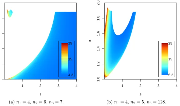
(Schlather et al., 2017). Figure 3.1 provides an example of the maximum attainable |ρ| in inequality (3.22) that have been found numerically. For details on implementation see Sec-tion 5.2.

(38)

Figure 3.1: The maximum attainable|ρ|in inequality (3.22) for the bivariate powered exponential covariance model in R. The

parameters areα11= 0.2, α22= 0.5,s11=

2, s22= 3.

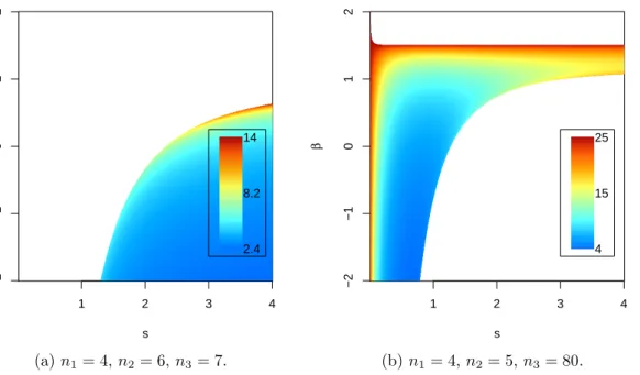
Figure 3.2: The maximum attainable|ρ|in inequality (3.30) for the bivariate Cauchy covariance model inR. The parameters are

α11 = 0.5, α22 = 0.9, β11 = 2, β12 = 2.5,

β22= 2.1,s11= 2, s22= 2.5.

3.5 Bivariate generalized Cauchy model

The univariate generalized Cauchy model,

ψ(r|α, β, s) = (1 + (sr)α)−β/α,

has been introduced in Gneiting (2000); Gneiting and Schlather (2004). Heres >0 is a scale parameter,α∈(0,2] is a smoothness parameter andβ >0 controls the long range behaviour of the field. The model was applied to many fields of science and technology, including network traffic (Li and Lim, 2008), hydrology (Koutsoyiannis, 2005) and medicine (Muniandy and Stanslas, 2008).

Each marginal covariances of the bivariate generalized Cauchy model,

Cii(r) =σ₁2(1 + (siir)αii)−βii/αii, (3.28) is of generalized Cauchy type with variance parameter σi, smoothness parameter αii ∈(0,2], long range parameterβii>0 and scale parameter sii>0,i= 1,2.Each cross covariance,

C12(r) =C21(r) =ρσ1σ2(1 + (s12r)α12)−β12/α12, (3.29)

is also of generalized Cauchy type with the colocated correlation coefficient ρ, smoothness parameterα12∈(0,2], long range parameterβ12>0 and scale parameter s12>0.