Estimating Long Term Equity Implied Volatility

(1)

Estimating Long Term Equity Implied Volatility

Danielle Ana Crawford

A dissertation submitted to the Faculty of Commerce, University of Cape Town, in partial fulfilment of the requirements for the degree of Master of Philosophy.

June 23, 2019

MPhil in Mathematical Finance, University of Cape Town.

University

of

Cape

(2)

The copyright of this thesis vests in the author. No

quotation from it or information derived from it is to be

published without full acknowledgement of the source.

The thesis is to be used for private study or

non-commercial research purposes only.

Published by the University of Cape Town (UCT) in terms

of the non-exclusive license granted to UCT by the author.

University

of

Cape

(3)

Declaration

I declare that this dissertation is my own, unaided work. It is being submitted for the Degree of Master of Philosophy in the University of the Cape Town. It has not been submitted before for any degree or examination in any other University.

(4)

Abstract

Estimating and extrapolating long term equity implied volatilities is of importance in the investment and insurance industry, where ’long term’ refers to periods of ten to thirty years. Market-consistent calibration is difficult to perform in the South African market due to lack of long term liquid tradable derivatives. In this case, practitioners have to estimate the implied volatility surface across a range of ex-piries and moneyness levels. A detailed evaluation is performed for different es-timation techniques to assess the strengths and weaknesses of each of the mod-els. The estimation techniques considered include statistical and time-series tech-niques, non-parametric techniques and three potential methods which use the local volatility model.

(5)

Acknowledgements

I would like to express my deep gratitude to Obeid Mahomed, my research su-pervisor. I am grateful for his patience, guidance, useful critiques and immense knowledge he provided throughout my dissertation. Furthermore, I would like to thank the lectures at AIFMRM for the valuable courses that provided me with the skills to be able to complete this dissertation. Lastly, I would like to thank the Banking Sector Education and Training Authority (BANKSETA) for the financial support they provided.

(6)

List of Figures

2.1 Historical terminal realised volatility usingτ-period returns. . . 7

2.2 Historical path-wise realised volatility usingτ-period returns. . . 8

2.3 EWMA monthly terminal volatility using overlapping and non-overlapping monthly returns. . . 9

2.4 EWMA monthly path-wise volatility using overlapping and non-overlapping monthly returns. . . 9

2.5 Volatility estimates using non-overlapping daily returns with vary-ingτ. . . 10

2.6 GJR-GARCH(1,1) volatility forecasts.. . . 11

2.7 Comparison between historical and implied volatilities for a range of maturities.. . . 12

2.8 Average IVHV Ratios for the JSE Top40 Index from 2010-2018. . . 13

3.1 Volatility estimates using Canonical Valuation with increasing GBM sample size while applying different sampling techniques. . . 18

3.2 Volatility skew using Canonical Valuation while applying different sampling techniques using GBM data. . . 19

3.3 Profit and loss profile of a three month at-the-money call option us-ing one thousand years of simulated GBM price data withσ= 30%. . 20

3.4 Volatility estimates using Break-Even volatility with increasing GBM sample size while applying different sampling techniques. . . 21

3.5 Volatility skew using Break-Even volatility while applying different sampling techniques using GBM data. . . 22

3.6 Volatility estimates using Canonical Valuation with increasing Hes-ton sample size while applying different sampling techniques. . . 23

3.7 Volatility skew using Canonical Valuation while applying different sampling techniques using Heston data. . . 24

3.8 Volatility estimates using Break-Even volatility with increasing Hes-ton sample size while applying different sampling techniques. . . 25

3.9 Volatility skew using Break-Even volatility while applying different sampling techniques using Heston data. . . 26

3.10 Volatility estimates using Canonical Valuation with increasing Mer-ton sample size while applying different sampling techniques. . . 27

3.11 Volatility skew using Canonical Valuation while applying different sampling techniques using Merton data. . . 28

3.12 Volatility estimates using Break-Even volatility with increasing Mer-ton sample size while applying different sampling techniques. . . 28

(9)

3.13 Volatility skew using Break-Even volatility while applying different sampling techniques using Merton data. . . 29

4.1 JSE Top40 volatility surfaces on the 20/11/17.. . . 33

4.2 Implied volatility estimates using Method 1 for JSE Top40 at-the-money European call. . . 34

A.1 Volatility estimates using Canonical Valuation with GBM data while applying different sampling techniques with the same Monte Carlo estimates.. . . 43

A.2 Volatility estimates using Break-Even volatility with GBM data while applying different sampling techniques with the same Monte Carlo estimates.. . . 44

A.3 Volatility estimates using Canonical Valuation with Heston data while applying different sampling techniques with the same Monte Carlo estimates.. . . 45

A.4 Volatility estimates using Break-Even with Heston data while apply-ing different samplapply-ing techniques with the same Monte Carlo esti-mates.. . . 45

A.5 Volatility estimates using Canonical Valuation with Merton data while applying different sampling techniques with the same Monte Carlo estimates.. . . 46

A.6 Volatility estimates using Break-Even volatility with Merton data while applying different sampling techniques with the same Monte Carlo estimates.. . . 47

(10)

List of Tables

2.1 Average IVHV Ratios for JSE Top40 Index from 1996-2018. . . 13

B.1 Heston parameters used in Chapter 3. . . 48

B.2 Merton parameters used in Chapter 3. . . 49

(11)

Chapter 1 Introduction

The ability to estimate and extrapolate implied volatilities is critical to the insur-ance industry. This is due to the complex nature of long-term savings, retirement and investment products, offered by insurance companies, which incorporate em-bedded financial derivatives. In the insurance and investment industry ’long term’ refers to periods of ten to thirty years. There is a lack of liquid tradable deriva-tives with long enough expiries to facilitate market-consistent calibration for the purposes of pricing and hedging of insurance investment products. This is par-ticularly true in the South African market, where there are few long term traded instruments (Flint et al.,2014). In this case, practitioners have to resort to extrap-olating implied volatility surfaces which are defined across a range of strikes and expiries. It is recommended by current legislative and advisory practice notes1 to use market-consistent models; these are models that can reproduce market prices as closely as possible (Flintet al.,2014).

Flintet al.(2014) extensively covers commonly used implied volatility models, applying South African market data to these models. The objective ofFlint et al. (2014)’s study is to accurately estimate long term implied volatility while using market consistent models. This dissertation reviews the ability of these commonly used techniques to estimate or extrapolate long term implied volatility using statis-tical and time-series techniques in Chapter 2 as well as non-parametric techniques in Chapter 3, both of which are covered inFlintet al.(2014). To extend on the re-search done byFlintet al. (2014), potential solutions using a local volatility model are proposed and reviewed.

1_{Actuarial Society of South Africa. APN 110: Allowance for Embedded Investment Derivatives,}

Version 4. Advisory Practice Note, 2012. Actuarial Society of South Africa. Market Consistent Cali-bration in South Africa. APN 110 sub-committee presentation, 2010

(12)

Chapter 1. Introduction 2

This study will be done in three sections, each describing different estimation tech-niques:

1. Statistical and Time-Series Techniques: Methods which only require histor-ical time-series data to estimate volatility. The three methods considered are historical volatility, GJR-GARCH and exponentially weighted moving aver-age. These methods do not directly estimate implied volatility.

2. Non-Parametric Techniques: Methods which only require historical time-series data to estimate fair volatilities. The two non-parametric methods con-sidered are Canonical Valuation and Break-Even volatility. These methods directly estimate implied volatility.

3. Potential Solutions Using a Local Volatility Model: These methods require cross sectional option data. Three models are considered which make use of the Local Volatility model. These models directly estimate implied volatility. This dissertation will include a detailed evaluation of each model’s ability to estimate the entire implied volatility surface. Furthermore, it will investigate the ability of each model to extrapolate the implied volatilities that are not readily ob-servable in the market (i.e for non-existing long dated options). Various features regarding each model are evaluated. These features include the data requirements, type of volatility estimated, if term structure estimation is possible, if skew estima-tion is possible across a range of moneyness levels, if statistical confidence inter-vals for the volatility estimates are possible to construct and the sensitivity of the volatility estimate to new data. The analysis is performed using both simulated and real-world data. Data is simulated using geometric Brownian motion (GBM), Heston (Drgulescu and Yakovenko,2002) and Merton models (Linghao,n.d.). The FTSE/JSE Top40 Index is the most liquid in the South African equity market thus this data is used in the analysis. The JSE Top40 Index data set used in this paper includes daily spot index levels spanning a 22.75 year period from 30 August 1995 to 29 April 2018 and option implied volatilities for a range of expiries.

In the analysis which follows, the underlying asset price at timet will be de-noted by the variableSt. The τ-period log-return of the underlying asset will be denoted as follows: rt,τ =ln St S(t−τ) . (1.1)

The holding period of the asset is from (t−τ) totresulting in one log-return over theτ-period. It is assumed throughout this dissertation thatτ is expressed in terms of business days, with 21 business days in a month and 252 business days in a year (Flintet al.,2012).

(13)

Chapter 2 Traditional Estimation Techniques

Market implied volatility data can be sparse. In this case, techniques which use only historical time-series data of the underlying asset can be used. These esti-mation techniques result in historical volatility estimates which need to be scaled to produce an appropriate implied volatility estimate. A commonly used scaling factor is referred to as the implied volatility historical volatility (IVHV) ratio (Flint

et al.,2014). The estimation techniques that will be considered can be categorised as follows:

(i) Statistical Techniques (ii) Time-Series Techniques

These techniques use different assumptions to characterize the underlying asset’s data generating process.

2.1 Historical Volatility

Historical volatility, also referred to as statistical volatility, is often defined as the standard deviation of the log-returns of an asset. This method of calculating volatil-ity is more commonly known as sample standard deviation and assumes that fu-ture volatility will follow the same path as historical volatility. The estimate is usu-ally annualised by multiplying the sample variance of return data by252_τ , where 252 is the assumed number of business days in a year andτ is the number of business days in the period under consideration. The important variables to consider in this calculation are the length of the sampling period (τ) and the number of sampling periods (n). It is important to ensure that the asset returns are non-overlapping, and independently and identically distributed (i.i.d.). Given the latter, classical his-torical volatility is defined as:

ˆ σ(t, τ, n) = v u u t 252 τ 1 n−1 n X i=1 r₍_t_i_,τ₎−¯r(t, τ, n)2 , (2.1)

where ¯r(t, τ, n) = 1_nPn_i₌₁r₍_t_i_,τ₎ is the average τ-period asset return andt is the current timetn(Figlewski,1994). The resultant volatility estimates the deviation of theτ-period returns from the averageτ-period return. An alternative to equation

(14)

2.2 EWMA Volatility 4

(2.1) is known as historical realised volatility where the average asset return is not subtracted from the return values or rather, is assumed to be zero (Flintet al.,2014):

ˆ σ(t, τ, n) = v u u t 252 τ 1 n−1 n X i=1 r(ti,τ) 2 . (2.2)

Equation (2.2) is more commonly used to calculate historical volatility. This method assumes that the meanτ-period return is zero. Thus, realised volatility is generally used when the average returns are close to zero. Assuming the mean return is zero will avoid errors caused by estimating the mean, this is especially prevalent for short periods. Historical realised volatility estimates may be more reliable than classical historical volatility (Ederington and Guan,2006).

It is common in academic literature to consider daily returns over a τ-period when estimating the volatility for derivative pricing (Flintet al.,2012). Given daily asset returns the sample historical volatility is given by:

ˆ σ(t,1, τ) = v u u t(252) 1 τ −1 τ X i=1 r(ti,1)−¯r(t,1, τ) 2 . (2.3)

where r¯(t,1, τ) is the one day average asset return for the τ-period under con-sideration. The resultant volatility estimate using equation (2.3) can be described as a path-wise estimate. This is because the volatility estimate for the τ-period will depend on the daily returns in theτ-period. Equation (2.1) results in a ter-minal volatility estimate where only τ-period returns are considered. It should also be considered if each volatility estimate will use overlapping (rolling) or non-overlapping (blocked) price data. Overlapping data estimates are advantageous when there is a lack of price data but results in biased volatility estimates due to auto-correlation in the overlappingτ-period return data.

Historical volatility is a simple method for forecasting the volatility of stock price returns. Implied volatility is not calculated directly when using historical volatility methods and therefore needs to be scaled with an estimated IVHV ratio. This estimating technique has been criticised for assuming that future volatility will follow the same path as historical volatility. To forecast thirty year implied volatility using equation (2.1), thirty years of historical stock price data are needed for just one estimate. This is also true for the path-wise volatility estimate where thirty years of daily returns are needed for the thirty year volatility estimate. These amounts of data are not always available therefore this forecasting technique may not be viable. This estimation technique has also been criticised for weighting all historical returns equally irrespective of how far the data extends into the past ( Ed-erington and Guan,2006).

2.2 EWMA Volatility

The idea behind the exponentially weighted moving average (EWMA) model is that data that is more recent influences the volatility forecasts more than data that

(15)

2.3 GARCH Volatility 5

are further in the past. This is enforced in the model by weighting more recent events higher than those in the past (Korkmaz and Aydin, 2002). This method improves on the estimates of equation (2.3), where daily return data equally con-tributes to the volatility estimate. It is assumed that the mean return of the data are zero and the returns are i.i.d. The EWMA volatility forecast at timetis:

σt= v u u t(1−λ) n−1 X i=0 λi−1_r2 (t−i,1), (2.4)

whereλ, referred to as the decay parameter, is a constant between 0 and 1,r(t−i,1)

is the log-return at time (t−i) andnis the number of historical observations under consideration. The larger theλ parameter the more influence the recent returns will have on the volatility estimate. The optimalλ value can be found using an optimization method decribed byLadokhin(2009). Equation (2.4) can be reduced to the following recursive form:

σ_t2=λσ2₍_t₋₁₎+ (1−λ)r2₍_t,₁₎, (2.5) where the next period’s varianceσ2_t depends on the current period’s varianceσ₍2_t₋₁₎

and returnr(t,1). It is recommended byKorkmaz and Aydin(2002) to useλ= 0.94

for daily volatility forecasting and 0.97 for monthly volatility forecasting (Vieira

et al., 2012). Again, the resultant volatility estimate needs to be scaled by an ap-propriate IVHV ratio to obtain the implied volatility estimate. The disadvantage of the EWMA method is that the method does not capture asymmetry1in volatility. Another model shortcoming is that it is assumed that returns are i.i.d., which has been empirically proven to be incorrect (Ederington and Guan,2006).

2.3 GARCH Volatility

The generalised autoregressive conditional heteroscedasticity, GARCH(p,q), model is a standard model used to capture market features. These features are statistical properties commonly seen in market data which include heavy-tailed distributions, skewed distributions, volatility clustering and volatility feedback effects 2 (Flint

et al.,2014). These stylised features oppose the fundamental assumption that asset returns are i.i.d, therefore the GARCH model is a suitable model to capture these market features. These models are autoregressive models in squared returns of the data, meaning that the current return is dependent on past returns. The conditional term describes that the volatility of the following period is conditional on the fea-tures of the current period. Heteroscedasticity describes the varying volatility of each period in the time-series data (Reider,2009).

1_{Volatility tends to be higher in periods where returns are decreasing than in periods where}

re-turns are increasing.

(16)

2.4 Overlapping vs. Non-Overlapping Returns 6

The model assumes the daily return on an asset or portfolio is:

rt,1 =E[rt,1|F(t−1)] +t (2.6)

t=σtzt, (2.7)

where the mean return is conditional on all past information up to (t−1), denoted by F₍_t₋₁₎, and {zt} are i.i.d. N(0,1)random variables for the standard GARCH model. The variablet is the residual return (AL-Najjar, 2016). The conditional variance is defined as:

σ2_t =ω+ p X j=1 αj2(t−j)+ q X k=1 βkσ(2t−k). (2.8)

There are many forms of the GARCH model in which the model features are spec-ified differently. These features include the functional form of the conditional vari-ance equation, the distribution of{z(t)}and the number of lags or choice of param-eterspandq. The GARCH(1,1) model is the most popular volatility model used for financial time-series data with parameters: p = 1,q = 1,ω > 0,α1 >,β1 >0and

α1+β1 < 1. It is recommended byFlintet al.(2014) to use the GJR-GARCH(1,1)

model with student-t innovations for the daily JSE Top40 dataset:

σ_t2=ω+ [α+γI(t−1)<0]

2

(t−1)+βσ2(t−1), (2.9)

whereI(t−1)<0is the indicator function which is one when(t−1) <0(Hansen and

Lunde,2005).

This model accounts for asymmetric volatility due to positive and negative re-turn shocks, which the GARCH(1,1) model does not. Theγparameter controls the effects of the asymmetric features in the data such that negative shocks result in the addition ofα+γ whereas positive shocks result in the addition ofα. Ifγ > 0, negative shocks will have a larger influence on the volatility estimate and ifγ < 0

positive shocks will have a larger effect (Liu and Hung,2010). The parametersω,α

andβmust all be non-negative. It is also required thatα+β+ 0.5γ <1andα+ 0.5γ

must be positive (Liu and Hung,2010).

2.4 Overlapping vs. Non-Overlapping Returns

The first data consideration is if overlapping or non-overlapping returns should be used when calculating the volatility estimate. Using overlapping returns is advan-tageous when there is a lack of stock price data as it artificially creates more return data. In this case, the return data used for eachτ-period would overlap with the prior period by (N−1), such that there areN returns in each period. For example, if there are two weeks of stock price data available and weekly volatility is estimated then non-overlapping returns would result in two stock price returns for the two week period whereas overlapping returns would result in six stock price returns.

Using overlapping returns may be beneficial but it may not be suitable for the estimation technique in use. Historical volatility and EWMA methods assume the

(17)

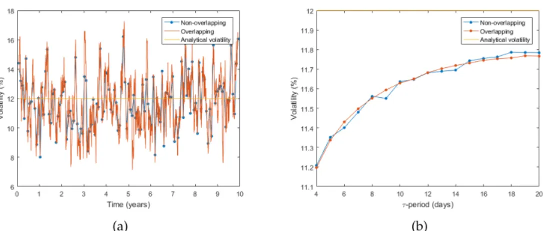
Fig. 2.1:Historical terminal realised volatility usingτ-period returns.

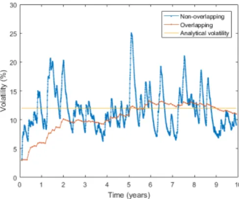
return data are i.i.d. By using overlapping returns this will induce auto-correlation between returns therefore breaking the assumption that returns are independent. To illustrate this, consider ten years of simulated GBM data. Equation (2.2) is im-plemented to estimate historical realised volatility forτ-periods increasing from a week to a month, as seen in Figure2.1. This figure illustrates the effect of using overlapping and non-overlappingτ-period returns on the volatility estimate. Us-ing overlappUs-ing returns results in more volatile estimates that deviate more from the analytical solution in comparison to using non-overlapping returns, consequen-tially leading to less accurate estimates. Figure2.2(a)illustrates the effect of using overlapping or non-overlapping returns on the volatility estimate using the histor-ical volatility path-wise estimation technique, as seen in equation (2.3). Monthly volatility is estimated iteratively through the ten years of simulated GBM data. Since, in the overlapping case, each volatility estimate uses (τ - 1) returns from the prior period, the volatility estimates are correlated. The non-overlapping technique results in volatility estimates which coincide with the overlapping estimates when the periods coincide. Figure2.2(b) illustrates the average non-overlapping path-wise estimates for varyingτ-periods. The estimates are dependent on the stock price path. There is little variation between the overlapping and non-overlapping estimates3. The path-wise historical estimation technique using daily returns re-sults in volatility estimates that are not very sensitive to the use of overlapping or non-overlapping data.

To illustrate the same effect, now using the EWMA estimation technique, con-sider ten years of simulated GBM data. Equation (2.5) is used to estimate EWMA monthly volatility using overlapping and non-overlapping return data for the monthly-periods under consideration. Monthly volatility is calculated throughout the ten years of simulated data using consecutive monthly periods. Since monthly volatil-ity is being estimated λ = 0.97 is used. Figure 2.3 illustrates the effect of us-ing overlappus-ing returns in the volatility calculation in comparison to usus-ing non-overlapping returns. Using non-overlapping returns results in more volatile volatility 3_{The values of the parameters in this example has resulted in the underestimation of the volatility.}

It cannot be concluded that the pathwise volatility estimate will always underestimate the volatility regardless of the size of parameters as this is not always the case.

(18)

(a) (b)

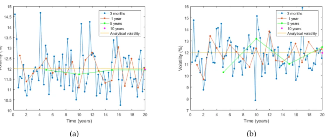
Fig. 2.2:Historical realised volatility usingτ-period returns. (a)Path-wise volatil-ity estimates withτ equal to one month. (b)Average path-wise volatility estimates for varyingτ-periods.

estimates which consequently leads to less accurate estimates. This is confirmed by comparing the analytical volatility to the estimated volatility by measuring the Root Mean Squared Error (RMSE)4 of the estimates (Chai and Draxler,2014). The RMSE of the volatility estimates using overlapping returns is higher than that of the non-overlapping returns. Figure 2.4(a)illustrates the effect of using overlap-ping or non-overlapoverlap-pingτ daily returns on the path-wise volatility estimates using equation (2.4). Using overlapping returns results in more volatile estimates in com-parison to using non-overlapping daily returns. The non-overlapping estimates coincide with the overlapping estimates when theτ-period coincides. Path-wise volatility estimates tend to be smaller than the analytical solution. This is due to the sample sizeτ. Figure2.4(b)illustrates the average EWMA volatility estimate using varyingτ daily returns. The non-overlapping and overlapping techniques result in volatility estimates which do not differ greatly. The volatility estimate is dependent on the path of the return data.

It is important to ensure that the return data used, when estimating volatility with techniques that assume the return data is i.i.d., is not overlapping. Using overlapping returns will result in an autocorrelated series of returns which contra-dicts the assumptions of the model, leading to less accurate estimates. This is of particular importance when a terminal estimation technique is used. Since stock price returns are known to not be i.i.d. the GARCH model may be a more suitable alternative to the historical and EWMA models.

4_{This method is used to measure the accuracy of the estimates by calculating the square-root of}

(19)

Fig. 2.3:EWMA monthly terminal volatility using overlapping and non-overlapping monthly returns.

(a) (b)

Fig. 2.4:EWMA monthly path-wise volatility using overlapping and non-overlapping monthly returns. (a) Path-wise volatility estimates with τ

equal to one month. (b)Average path-wise volatility estimates with vary-ingτ.

(20)

2.5 Data Sample Size 10

(a) (b)

Fig. 2.5:Volatility estimates using non-overlapping daily returns with varying τ.

(a)Historical realised volatility.(b)EWMA volatility.

2.5 Data Sample Size

The second data consideration is the size of the data sample used for the volatility estimate. Different estimation techniques require different amounts of data to en-sure accurate estimates. Thus, it is important to assess how much data is needed for the estimation technique under consideration.

Term structure estimation is possible using historical or EWMA methods by varying the sample size or by obtaining the volatility estimate and then using the square-root of time rule. It is possible to use the square-root of time rule because these volatility estimation techniques assume the asset returns are i.i.d. The path-wise estimation techniques using daily non-overlapping returns are considered in this analysis.

Realised volatility estimates with varyingτ-periods are shown in Figure2.5(a)

using twenty years of simulated GBM data. The smaller theτ-period the greater the variability in the volatility estimates. Therefore, calculating volatility using larger periods leads to more accurate results when forecasting long-term volatility. Smallerτ-periods are more sensitive to outliers in the data whereas largerτ-periods are less effected by sampling period (Ederington and Guan,2006). The larger theτ -period the more normal the distribution of the return data, due to the central limit theorem.

The decay parameterλused in the EWMA method is dependent on the size of

τ. Greaterτ-periods require larger decay parameter values. Figure2.5(b)illustrates the term structure estimation for twenty years of simulated GBM daily stock price data with varyingτ-periods. Shorterτ-periods are more sensitive to return shocks than longerτ-periods.

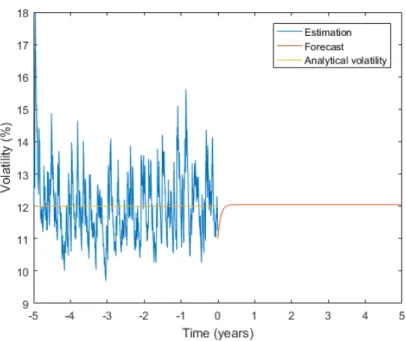
Term structure estimation is possible using GARCH models. Once a GARCH model is fitted to the return data, term structure specification is possible for volatil-ity forecasts. To illustrate this, five years of daily GBM stock price data is simulated to calculate daily GJR-GARCH(1,1) volatility using student-t innovations. The

(21)

Mat-2.6 IVHV Ratios 11

Fig. 2.6:GJR-GARCH(1,1) volatility forecasts.

lab functionestimateis used to estimate the parameters in equation (2.9). These pa-rameters are used as an input to the Matlab functionforecastwhich forecasts daily volatility andinferwhich infers conditional variances. Figure2.6displays the daily GJR-GARCH(1,1) inferred volatility and volatility forecasts for the simulated GBM stock prices. It is important to note that the volatility forecasts do not change sig-nificantly after four months as seen in Figure2.6. The estimates after four months are very close to the given volatility of12%. In this case since the data is i.i.d. the GJR-GARCH(1,1) model results in a good estimate of the long term volatility. Typ-ically the GJR-GARCH(1,1) model is used to forecast volatility from one month to one year. The fitted model may not be suitable for forecasting long term volatility (Flintet al.,2014).

2.6 IVHV Ratios

Historical volatility forecasts future volatility based on past values, whereas im-plied volatility is the markets view on what future volatility will be; these two volatility estimates differ. This difference is called the volatility premium. Im-plied volatility is known to generally be higher than historical volatility (Eraker,

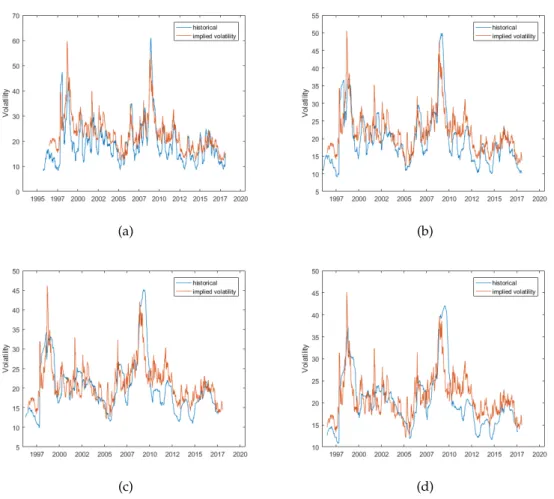
2008). Daily log-returns of the JSE Top40 Index levels are used to estimate histor-ical volatility for one, three, six, nine and twelve month periods; these values are compared to market implied volatilities, for at-the-money options, to calculate the IVHV ratio.

(22)

ex-2.6 IVHV Ratios 12

(a) (b)

(c) (d)

Fig. 2.7:Comparison between historical and implied volatilities for a range of ma-turities.(a)3 months.(b)6 months.(c)9 months.(d)1 year.

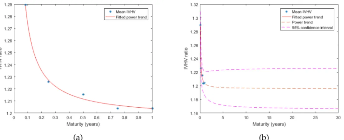
piries from 1996 to 2018. The implied volatilities for at-the-money options on the JSE Top40 Index are predominantly higher than historical volatility for each of the expiries. The average IVHV ratio for each term is above one, as seen in Table2.1. The IVHV ratio fluctuates over time as seen in Figure2.7. In high volatility pe-riods i.e. 2008 financial crisis, the implied volatilities are smaller than historical volatilities for each maturity. There is a decrease in IVHV ratio with an increase in maturity with the exception of twelve months, due to the lack of data. A power trend is fitted to the mean IVHV ratios for the JSE Top40 Index from 2010-2018, as seen in Figure2.8(b) (Flint et al., 2014). The 5% and 95% confidence intervals for the IVHV ratio is used to scale resultant volatility estimates for different expires. This results in an implied volatility range for a given maturity, rather than a point estimate.

It is not possible to directly estimate implied volatility for options that are in- or out-the-money when using the traditional estimation techniques described. Thus, volatility skew or smile can only be estimated by scaling historical volatility esti-mates by in- or out-the-money IVHV ratios to obtain implied volatility skew per maturity.

(23)

2.6 IVHV Ratios 13

1 month 3 months 6 months 9 months 12 months Mean 1.3401 1.2443 1.1488 1.0989 1.0882 Median 1.2928 1.2328 1.1358 1.0961 1.0972

Tab. 2.1: Average IVHV Ratios for JSE Top40 Index from 1996-2018.

(a) (b)

Fig. 2.8:Average IVHV Ratios for the JSE Top40 Index from 2010-2018.(a)Average IVHV Ratios for the JSE Top40 Index fitted to a power trend. (b) Extrapo-lated IVHV Ratios for the JSE Top40 Index.

(24)

Chapter 3 Non-Parametric Techniques

Non-parametric methods are used to obtain market-consistent fair volatilities us-ing only historical market data. The two non-parametric methods used byFlint

et al. (2014) to estimate volatilities are Canonical Valuation (CV) and Break-Even volatility (BEV). This chapter explores these two methods and assesses their ability to estimate the implied volatility surface.

3.1 Canonical Valuation

Canonical Valuation is a non-parametric method which values derivatives under a risk-neutral framework. This pricing method only requires a series of historical stock prices. The underlying distribution of the stock price data over someτ-period is not assumed to be log-normal, as in the Black-Scholes framework, but rather uses an estimation of the distribution of historical returns to predict the risk-neutral distribution of asset prices at expiration (Gray and Newman,2005). This is done using the principal of minimum relative entropy. This pricing method is named after the Gibbs canonical distribution which is used to estimate the risk-neutral distribution (Stutzer,1996).

Once this distribution is estimated, a vanilla European option can be priced; these prices are then used to imply fair volatilities for theτ-period, such thatτ is defined asτ = [t0, T]. The risk-neutral value of an option at timet0, over the τ

-period, is given by the discounted present value of the pay-off of the option under the risk-neutral measure:

Vt0,T (ST) =Z(t0,T)E Q_[_V T|Ft0] =Z(t0,T) Z ∞ 0 VT π∗(ST)dST, (3.1) whereZ(t0,T)denotes the risk-free discount factor over the period[t0, T],EQ[·|·]is

the conditional expectation under the risk-neutral probability measureQ,VT is the value of the derivative at timeT andπ∗(ST)is the risk-neutral probability density function of the underlying asset price at expirationT (Flintet al.,2012).

In order to implement this pricing method consider a European call option ex-piring at timeT such that the current time ist0. Firstly, the real world probability

(25)

3.1 Canonical Valuation 15

of historical stock price returns. This is done by calculating a sample ofN τ-period asset returnsr₍_t_i_,τ₎ withi = 1, . . . , N, using equation (1.1) whereτ is equal to the length of the option. TheseN asset returns are used to calculate a series of possible future stock prices at expiration as follows:

S(Ti,τ) =S0e

r(_ti,τ)_, _i_{= 1}_{, . . . , N.} _(3.2)

whereS0is the current stock price ander(ti,τ) is the growth rate. Each of theS(Ti,τ)

values are allocated an equal real-world probability ofπˆ = _N1 (Alcock and Gray,

2005). This empirical distribution can be transformed into its risk-neutral coun-terpart π∗ on condition the following is satisfied to ensure arbitrage-free option pricing: Sti =E Q ti _S (Ti,τ) erτ = EPti _S (Ti,τ) erτ dπ∗ dˆπ , (3.3)

whereris the risk-free rate and dπ_d_π_ˆ∗ is the Radon-Nykodym derivative of the risk-neutral measure with respect the real world measure. The superscript of the ex-pectation indicates which probability measure is used to calculate the exex-pectation. Equation (3.3) can be simplified to:

1 = N X i=1 e−rτ X(ti,τ) π∗_i ˆ πi ˆ πi, (3.4)

whereX₍_t_i_,τ₎=er(_ti,τ) _and_π∗

i is the risk-neutral probability of returnr(ti,τ)(Stutzer, 1996). Equation (3.4) ensures that the martingale property is satisfied and the dis-counted expected return on the stock sums to one (Alcock and Gray, 2005). The risk-neutral distribution can be estimated using the method of relative entropy which minimizes the difference between the empirical distribution and risk-neutral probability distribution of the underlying. Since the pay-off of the option depends on the terminal stock price, estimating the distribution of the underlying stock price is beneficial as stylized features in the data may be captured (Gray and Newman,

2005). The following relative entropy (RE) expression should be minimized to solve forπ∗_i: RE(π_i∗,πˆi) = N X i=1 π_i∗log π∗_i ˆ πi s.t.(3.4). (3.5)

The solution to this convex minimization problem is given by the Gibbs canonical distribution: π_i∗ = exp γ ∗_e−rτ_X (ti,τ) PN i=1exp γ∗e−rτX(ti,τ) , (3.6)

such that the Lagrange multiplierγ∗satisfies the following:

γ∗ =argmin γ N X i=1 exp γ(e−rτX(ti,τ)−1) . (3.7)

(26)

3.2 Break-Even Volatility 16

The call option can be priced using the resulting risk-neutral probabilities, as fol-lows: Cτ(K) =e−rτ N X i=1 max[S₍_T_i_,τ₎−K,0]π_i∗. (3.8) The difference between equation (3.8) and the Black-Scholes price is then set to zero to solve for the implied volatility (Stutzer,1996).

3.2 Break-Even Volatility

Break-Even volatility is defined as the volatility, for a delta-hedged option, which results in zero profit and loss. This method is based on dynamic replication such that a portfolio consisting of an underlying asset and cash is used to replicate an op-tion over aτ-period. Assuming the standard Black-Scholes framework, this delta-hedge will result in a profit and loss function which is set to zero by solving for the corresponding implied volatility. The profit and loss of a continuously delta hedged option is the gamma-weighted average of past quadratic returns:

P&L= Z T 0 1 2ΓuS 2 u[σu−σimp2 ]du (3.9) whereσimp=σ(t0,τ)is the fair implied volatility of the option over theτ-period,Γis

the standard Black-Scholes gamma of the option andσuthe instantaneous realised volatility (Flint et al.,2014). Equation (3.9) can be approximated by the following discrete profit and loss equation:

P&L(t0, T, σimp) = 1 2 τ X i=1 erτΓtiS 2 ti[r 2 (ti,1)−σ 2 imp∆t], (3.10)

whereerτ is the risk-free capitalization factor over theτ-period and∆t =

ti−t(i−1)

365

(Flintet al.,2014). Assuming the current time ist0with the option expiring at time

T, hedging of the option occurs discretely at times {t0, t1, ..., T}. It is suggested

byFlint et al. (2014) to solve for the volatility that ensures the average P&L over the different time periods is zero; this results in a smoother volatility surface than the alternative, averaging the volatilities that results in zero P&L for each time pe-riod. Each returns period is rebased using the initial stock price,S0. This results in

a smoother volatility surface with the consequence of considering relative strikes instead of absolute strike values (Dupire,2006).

3.3 Data Sample Size

The first data consideration is assessing how much data is required for both CV and BEV methods to recover accurate results. Using real world stock price data is restrictive for this study as these methods are computationally intensive requir-ing a large amount of data to produce reasonable results. Thus, stock price data

(27)

is simulated using GBM. Using simulated GBM data is useful for testing the accu-racy of the volatility estimates, as the GBM model assumes volatility is constant. Since using non-overlapping returns may result in too fewτ-period returns, over-lapping and statistical bootstrapping methods are considered as ways to increase the sample size.

3.3.1 Canonical Valuation Implementation

Daily stock prices are simulated and implemented to calculate an array ofτ-period returns. By applying the Matlab functionfmincon, these returns are then used to calculate the Lagrange multiplier. The risk-neutral probabilities are then estimated using equation (3.6). Call options are priced using CV across a range of expiries and moneyness levels. The Matlab functionfzerois used to set the difference between the Black-Scholes price and the CV price to zero, to solve for the implied volatility. To demonstrate the impact of the data sample size on the implied volatility esti-mates consider using CV to estimate the implied volatility of a three month at-the-money (ATM) call option using simulated GBM data, with an analytical implied volatility of 30%. The analysis is done using non-overlapping, overlapping and statistical bootstrapping methods:

(i) Non-Overlapping Returns: Daily stock prices are simulated and used to cal-culate an array of non-overlappingτ-period returns, whereτ is three months. This results in a set of i.i.d. τ-period returns.

(ii) Overlapping Returns: Daily stock prices are simulated and used to calculate an array of overlapping τ-period returns, whereτ is three months. Eachτ -period return will overlap with the previousτ-period. This results in a set of

τ-period returns that are not i.i.d.

(iii) Statistical Bootstrapping: Daily stock prices are simulated and used to calcu-late an array of daily returns. A random sample ofτ returns is selected. This is repeated, with replacement, until there is a sufficient amount ofτ-periods. Throughout this chapter if the underlying data is i.i.d., the statistical bootstrap-ping method will result in estimates that are more accurate than using non-overlapbootstrap-ping returns. Since the data is i.i.d. statistical bootstapping will only result in a larger sample size, leading to more accurate results.

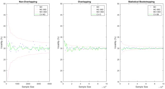
Figure3.1illustrates the impact the size of the return data has on the accuracy of the implied volatility estimates using the CV method while using non-overlapping, overlapping and statistical bootstrapping techniques. These estimates are com-pared to Crude Monte Carlo (MC) estimation and three standard deviation MC bounds. The amount of simulated GBM daily stock price data starts at twenty-five years increasing in twenty-five year increments to one thousand years. Implied volatility estimates using non-overlapping returns lie within the three standard de-viation MC bounds. A large amount of data is required to obtain very accurate results when using non-overlapping returns. Since using overlapping returns re-sults in returns that are not i.i.d, the implied volatility estimates are inaccurate,

(28)

thus not lying within the three standard deviation MC bounds. Despite this sam-pling method generating moreτ-period returns, it results in auto-correlated returns which will greatly bias the results. The statistical bootstrapping technique results in reasonable volatility estimates. This is due to the fact that the return data is i.i.d., therefore randomly selecting daily return data will not change the distribution of the returns. The CV method requires an immense amount of return data to pro-duce accurate results. In the event that there is a lack of stock price data and the data is i.i.d., statistical bootstrapping is a good alternative to using non-overlapping returns. The latter is emphasised in figureA.1found in AppendixA.

Fig. 3.1:Volatility estimates using Canonical Valuation with increasing GBM sam-ple size while applying different sampling techniques.

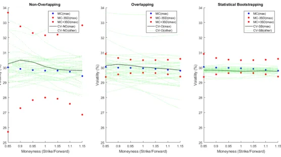
Since simulated GBM data is used in this analysis, the volatility across a range of moneyness levels is constant. Figure3.2illustrates the volatility skew for a three month option using one thousand years of simulated GBM data. The estimates are compared to MC estimates and three standard deviation MC bounds. The volatility estimates for twenty-five to nine-hundred and twenty-five years of simulated data is indicated asother. The statistical bootstrapping method results in the most consis-tent volatility estimates across the range of moneyness levels. The resultant volatil-ity skew using overlapping returns is more stable than using non-overlapping re-turns. Using non-overlapping return data results in unstable volatility estimates, particularly for in-the-money options.

(29)

Fig. 3.2:Volatility skew using Canonical Valuation while applying different sam-pling techniques using GBM data.

3.3.2 Break-Even Volatility Implementation

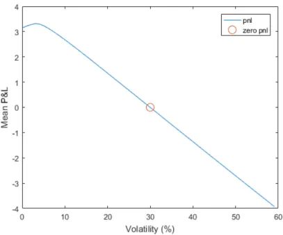
Daily stock prices are simulated and implemented to calculate an array of daily re-turns. Selectedτ-periods of daily returns are used to calculate theτ-period profit and loss using equation (3.10). Eachτ-period is rebased to ensure that the money-ness levels remain the same for every selectedτ-period. The Matlab functionfzero is used to find the volatility that ensures the average profit and loss for all the se-lectedτ-periods is zero. Figure3.3illustrates the average profit and loss, as a result of daily delta hedging, for a three month at-the-money call option using a range of volatilities. The BEV is 30%which is an accurate estimation of the analytical volatility of the simulated data.

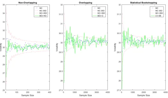
To demonstrate the impact of the data sample size on the implied volatility estimates, consider using BEV to estimate the implied volatility for a three month ATM call option using simulated GBM data, with an analytical implied volatility of 30%. The analysis is done using non-overlapping, overlapping and statistical bootstrapping methods as described in section3.3.1. Less simulated GBM stock price data is used as this method is more computationally intensive. Thus, one hundred years of GBM stock price data is simulated.

Figure 3.4 illustrates the impact the size of the return data has on the accu-racy of the implied volatility estimates using the BEV method while using non-overlapping, overlapping and statistical bootstrapping techniques. These estimates are compared to Crude MC estimation and three standard deviation MC bounds. Using non-overlapping returns results in BEV estimates of which the majority lie within the three standard deviation MC bounds. As the sample size is increased,

(30)

Fig. 3.3:Profit and loss profile of a three month at-the-money call option using one thousand years of simulated GBM price data withσ = 30%.

the implied volatility estimates become increasingly more stable and accurate. Us-ing overlappUs-ing returns results in volatility estimates with little variation between estimates but all the estimates do not lie within the three standard deviation MC bounds. The statistical bootstrapping technique results in a very similar estimate profile to that of overlapping returns, where the majority of the estimates lie within the three standard deviation MC bounds. The estimates using the overlapping and statistical bootstrapping techniques do not improve on the estimates using non-overlapping returns. This can also be seen in figure A.2 in Appendix A. If the number of years of simulated stock price data were to be increased, the increase in accuracy of the implied volatility estimates would become more apparent when using the overlapping and statistical bootstrapping methods.

Since simulated GBM data is used in this analysis, the volatility across a range of moneyness levels is constant. Figure3.5illustrates the volatility skew for an ATM call option using one hundred years of simulated GBM data. The estimates are compared to MC estimates and three standard deviation MC bounds. The volatil-ity estimates for one to ninety-nine years of simulated data is indicated asother. The non-overlapping method results in the volatility estimates which lie within the three standard deviation bounds across the range of moneyness levels. The resul-tant volatility skew using overlapping and statistical bootstrapping returns also lie within the bounds. All three sampling methods result in estimates that are unsta-ble for options that are deep in- or out-the-money. The estimates are unstaunsta-ble due to the short length of the option, thus there is a sparsity of paths that reach the specified moneyness level in the short time period.

(31)

Fig. 3.4:Volatility estimates using Break-Even volatility with increasing GBM sam-ple size while applying different sampling techniques.

BEV is computationally expensive in comparison to CV. This is due to the man-ner in which the implied volatility is estimated. Since the BEV method requires numerical optimization per strike for each maturity i.e. searching for the implied volatility which results in zero profit and loss, this is very computationally expen-sive in comparison to the alternative CV. When using the CV method only one numerical optimization is required per maturity to enable implied volatility esti-mation for a range of strikes. When using the CV method it is important to useτ -periods that are non-overlapping to ensure volatility estimates are accurate. In the case of the CV and BEV methods, if the daily return data is i.i.d., using the statistical bootstrapping method is a good alternative to using non-overlapping returns when there is a lack of stock price data. Term structure estimation is possible using both the CV and BEV techniques. Both the CV and BEV methods are able to estimate volatility skew, on the condition that a large amount of return data is used in the estimation. As the length of the option increases the number of non-overlapping

τ-period returns decreases which decreases the accuracy of the volatility estimate. Therefore the longer the length of the option the larger the amount of data is re-quired to obtain accurate results. Both the CV and BEV techniques require a large amount of stock price data for accurate volatility estimation.

(32)

3.4 I.I.D. Returns 22

Fig. 3.5:Volatility skew using Break-Even volatility while applying different sam-pling techniques using GBM data.

3.4 I.I.D. Returns

The assumption that the stock price process follows the Black-Scholes GBM dy-namics with a constant volatility has been found to be unrealistic. It has been found that returns are not normally distributed and contain fat tails (Drgulescu and Yakovenko,2002). For this reason, the Heston and Merton stochastic volatility models are considered and used to simulate stock price data. Since this simulated data may represent a more realistic stock price path, it will be used to assess the ability for the CV and BEV methods to estimate volatility and volatility skew. Over-lapping, non-overlapping and bootstrapping techniques are also considered as in Section3.3.

(i) Heston Model: The Heston model assumes volatility is stochastic therefore the resultant returns series is not i.i.d. See AppendixB.1for more information on the Heston model. See table B.1in AppendixB.1for the parameters used in the Heston model.

To illustrate the effect of non i.i.d. returns on the volatility estimates us-ing the CV method, consider one thousand years of simulated Heston stock price data. Figure 3.6illustrates the resultant volatility estimates for a three month ATM call option using the CV method. These estimates are compared to Crude MC estimation and three standard deviation MC bounds. The es-timates using overlapping and statistical bootstrapping techniques result in unstable volatility estimates, irrespective of the sample size. Thus, these two

(33)

sampling techniques are not effective methods to obtain more accurate results by increasing the sampling size. Although the use of non-overlapping returns results in estimates that are within the three standard deviation MC bounds, the estimates are unstable. The latter is emphasised in figureA.3in Appendix

A.

Fig. 3.6:Volatility estimates using Canonical Valuation with increasing Heston sample size while applying different sampling techniques.

Skew estimation can be seen in Figure3.7for a three month option. The CV technique using all three sampling techniques does not accurately estimate volatility skew, resulting in unstable estimates. Using non-overlapping re-turns results in volatility estimates that lie within the three standard devia-tion MC bounds whereas using non-overlapping and statistical bootstrapping techniques results in estimates which do not lie within these bounds.

To illustrate the effect of non-i.i.d. returns on the volatility estimates using the BEV method, consider one hundred years of simulated Heston stock price data. Figure3.8illustrates the resultant volatility estimates for a three month ATM call option using the BEV method with non-overlapping, overlapping and statistical bootstrapping techniques. These estimates are compared to Crude MC estimation and three standard deviation MC bounds. The mates using all three sampling techniques result in unstable volatility esti-mates, irrespective of the sample size. Thus, the BEV method is not capable of estimating volatility for stock price return data that is not i.i.d. The latter is emphasised in Figure A.4in AppendixA, where the MC estimates are the same for all three sampling techniques.

(34)

Fig. 3.7:Volatility skew using Canonical Valuation while applying different sam-pling techniques using Heston data.

The volatility estimates using the BEV method for a three month option at a range of moneyness levels is illustrated in Figure3.9. The estimates using all three sampling techniques result in unstable volatility estimates for a range of moneyness levels. Thus, the BEV method is unable to recover a volatility skew for return data that is not i.i.d.

The Heston model results in a returns series that is not i.i.d. Both CV and BEV methods do not perform well when the returns series is not i.i.d., resulting in unstable volatility estimates. Thus, the CV and BEV techniques may only be employed when the series of stock price returns is in-fact i.i.d.

(ii) Merton Model: The Merton model adds random jumps to the GBM dynamics to account for random stock price shocks. The resultant returns series remains i.i.d. See AppendixB.2for more information on the Merton model. See table

B.2in AppendixB.2for the parameters used in the Merton model.

To illustrate the effect of market data following the Merton model on the volatility estimates using CV and BEV methods, consider one thousand years of simulated Merton stock price data. Non-overlapping, overlapping and statistical bootstrapping techniques are used in this analysis. Figure 3.10 il-lustrates the volatility estimates using the CV method for a range of sample sizes. The volatility estimates are compared to MC simulation and three stan-dard deviation MC bounds. Using non-overlapping returns results in stable estimates that lie within the three standard deviation bounds. As the

(35)

sam-3.4 I.I.D. Returns 25

Fig. 3.8:Volatility estimates using Break-Even volatility with increasing Heston sample size while applying different sampling techniques.

ple size is increased there is less variation in the estimates. Using overlap-ping returns results in unstable estimates due to the autocorrelation in the returns. Using the statistical bootstrapping technique results in stable volatil-ity estimates. The variabilvolatil-ity in the estimates is decreased as the sample size increases thus, the statistical bootstrapping technique is a good alternative to increase the sample size. The latter is evident in FigureA.5in AppendixA. The volatility estimates using the CV method for a three month option at a range of moneyness levels is illustrated in Figure 3.11. The estimates us-ing all three samplus-ing techniques result in a volatility skew where the non-overlapping and statistical bootstrapping techniques result in estimates which lie within the three standard deviation MC bounds.

Figure3.12illustrates the volatility estimates using the BEV method for a three month ATM call option with a range of sample sizes using one hundred years of simulated Merton data. Using non-overlapping returns results in unstable volatility estimates of which the majority lie within the three standard devia-tion MC bounds. As the sample size is increased, the volatility estimates be-come more stable. Using statistical bootstrapping and overlapping techniques to increase the sample size does not result in an increase of the accuracy of the estimates. This is due to the immense amount of data that the BEV method requires to produce accurate results. The latter is emphasised in figure A.6

in Appendix A. If the number of years of stock price data were to increase, the statistical bootstrapping and overlapping sampling techniques would

(36)

im-3.4 I.I.D. Returns 26

Fig. 3.9:Volatility skew using Break-Even volatility while applying different sam-pling techniques using Heston data.

prove on the accuracy of the non-overlapping estimates.

Figure3.13illustrates the volatility estimates for a range of moneyness levels for a three month option using simulated Merton stock price data. Using non-overlapping returns results in volatility estimates which lie within the three standard deviation MC bounds. Using overlapping or statistical bootstrap-ping techniques results in estimates which also lie within these bounds. Thus, given i.i.d. return data and a large enough sample size the BEV method is able to recover a volatility skew.

The BE and CV methods result in satisfactory estimates provided the sample size is large enough and stock price returns series is i.i.d. If the stock price returns are i.i.d., the statistical bootstrapping method can be used to increase the sample size and is a good alternative to using non-overlapping returns when using the CV and BEV methods. Term structure estimation is possible using CV and BEV meth-ods. The disadvantage of the estimation techniques described is that the length of term structure is limited to the amount of available stock price data. Thus, longer maturities will result in unstable volatility estimates because of the lack of stock price data. Skew estimation is possible, as seen in the analysis using the Merton model to simulate stock price data, thus both the CV and BEV models are able to recover a skew when the data is i.i.d. Another drawback of these estimation tech-niques is that they only use equity stock price market data and no equity option market data. It is not possible to estimate statistical confidence intervals for the

(37)

Fig. 3.10:Volatility estimates using Canonical Valuation with increasing Merton sample size while applying different sampling techniques.

estimates. Lastly, these estimation techniques require the stock price returns series to be i.i.d. The i.i.d. condition may be unrealistic for market stock price returns.

(38)

Fig. 3.11:Volatility skew using Canonical Valuation while applying different sam-pling techniques using Merton data.

Fig. 3.12:Volatility estimates using Break-Even volatility with increasing Merton sample size while applying different sampling techniques.

(39)

Fig. 3.13:Volatility skew using Break-Even volatility while applying different sam-pling techniques using Merton data.

(40)

Chapter 4 Potential Solutions Using a Local

Volatility Model

The estimation procedures outlined in this chapter attempts to recover option prices at a given point in time. The models described are based on the SAFEX parametriza-tion proposed byKotz´e et al.(2015). The estimation techniques used can be cate-gorised as deterministic volatility models requiring a snapshot of option implied volatility data which directly models local volatility. Local volatility can be de-scribed as the instantaneous volatility at a specific point in time. Thus, local volatil-ity is time and state dependent (Kotz´eet al.,2015). Moreover, given a set of Euro-pean stock prices, there exists a unique risk neutral diffusion parameter, the local variance, which can be used to generate these prices (Gatheral and Lynch,2004).

Simulation techniques are used to extrapolate local volatilities for maturities that are unobservable in the market. Thus, the dynamics of the local volatility for maturities beyond what is observable in the market become partially stochastic in nature and are based on the assumptions used in the three proposed models de-scribed in this chapter. Since local volatility is dede-scribed as an instantaneous quan-tity, the proposed simulation extrapolation can be viewed as generating a partially stochastic volatility model for the asset price. The local volatility term structure is effectively reproduced and extended to unobservable maturities by extrapolation simulations of the existing local volatility surface. It should be emphasised that the existing local volatility surface is derived from a sample of market observable implied volatilities for a given range of maturities.

4.1 Local Volatility

Time-varying deterministic volatility models aim to create a volatility surface by fitting a deterministic model to an underlying stochastic asset-price process (Flint

et al.,2014). A popular non-parametric deterministic model considered is the local volatility model. This is a model in which volatility is a deterministic function of two variables, time (t) and the asset price at each time (St). Under the risk-neutral measure, the standard Black-Scholes framework assumes volatility is constant and asset prices follow a geometric Brownian motion:

(41)

4.1 Local Volatility 31

wherer is the risk-free rate and{Wt}denotes a standard Brownian motion under the risk neutral measureQ(Linghao,n.d.). In reality the assumption of constant volatility has been found to be inaccurate. Dupire has shown that the constant volatility in equation (4.1) can rather be modelled using the deterministic function

σ(t, St)which consequently adds some randomness to the volatility process (Davis,

2011). The randomness is added due to the dependence of the volatility on the stock price process, which is driven by Brownian motion. This results in a stock price process that will no longer have a constant volatility. The dynamics are described by:

dSt=rStdt+σ(t, St)StdWt. (4.2) Since there is still only one source of randomness in the model, the local volatility model is complete ensuring unique prices (Kamp,2009). The local volatility func-tionσ(t, St) is consistent with market prices of options on the underlyingS such thatσ(t, St)is the markets view of future volatility attwith stock priceSt.

The resultant local volatility may not be realised. Local volatility can be viewed as the average instantaneous volatility for a specified time and stock price hence the namelocal, whereas Black-Scholes implied volatility can be viewed as the overall globalfuture volatility for the lifetime of the option (Dermanet al.,1996). The local volatility can be extracted analytically from European option prices with Dupire’s formula for local volatility (Kotz´eet al.,2015):

σL(T, K) = v u u t ∂ ∂TC(St, T, K) +rK ∂ ∂KC(St, T, K) 1 2K2 ∂2 ∂K2C(St, T, K) , (4.3)

whereC(St, T, K)is the call price today andσL(T, K)is continuous. Local volatil-ity can be uniquely computed for a range of strike/asset prices and expirations using equation (4.3). It is assumed that the call price is twice differentiable with respect to the strike and once with respect to expiration. Since liquid option prices are only known for a discrete set of expiries and strikes, price data can be inter-polated to create a smoother price surface. It should be ensured that the option price function is convex with respect to strike to guarentee the second derivative in the denominator is postive and real. The derivatives can be approximated nu-merically using finite difference techniques (see appendix (C.2)) (Kotzeet al.,2014). It is suggested byKotzeet al.(2014) to use one to ten index points for the change in strike for the Top40 Index and one to ten basis points for the change in time. A percentage of the strike price could also be used while ensuring that it is small enough. There are a few areas which may result in errors using Dupire’s equation. Firstly, small absolute errors in the approximation of the second derivative in the denominator are magnified by the squared strike price. Secondly, this derivative will result in very small values for options deep in- or out-the-money, this is espe-cially prevalent for shorter termed options. An alternative method is to calculate local volatility in terms of market implied volatilities (Kotze and Oosthuizen,2015):

σL(St, T, K) = v u u u u t σ2 imp+ 2σimpT _∂σ imp ∂T +rK ∂σimp ∂K 1 + 2d1K √ T∂σimp ∂K +K2T d1d2 _∂σ imp ∂K 2 +σimp∂ 2_σ imp ∂K2 , (4.4)

(42)

4.2 Forecasting Using the Local Volatility Model 32 where d1 = ln St K +rT +σ 2 imp 2 T σimp √ T and d2 =d1−σimp √ T . (4.5)

The derivation of equation (4.4) is included in AppendixC.1. This method is more stable due to the elimination of the single standing dual Gamma in the denomina-tor. Small errors in the second derivative calculation will no longer lead to large overall errors, as they are now part of a summation rather than standing alone (Kotzeet al.,2014).

4.2 Forecasting Using the Local Volatility Model

In this section three methods are proposed as potential techniques for obtaining long-term equity implied volatility estimates. Local volatilities can be estimated us-ing equation (4.4) for a range of strikes and expiries where the maximum expiry is limited to what is observable in the market. The following three methods outlined are used to obtain implied volatilities for expiries longer than what is available in the market. Each method contains different assumptions about how future local volatility proceeds beyond what is observable in the market. In order to demon-strate these three methods consider an implied volatility surface with a range of strikesK and a range of expiries [t, t+dt, t+ 2dt, ..., T], wheredt is the interval between consecutive expiries. This implied volatility surface is applied to equation (4.4) resulting in local volatilities for the same range of strikes and expiries.

Given the local volatility surface, one of the three methods is applied to the local volatility data. Each of these methods comprises of an iterative process to forecast local volatility one step into the future. Once this local volatility is calculated, Mil-stein discretization is applied to equation (4.2) to obtain the stock price one time step into the future. This is performed iteratively until the desired number of stock prices are obtained. Monte Carlo simulation is performed with the resultant stock prices to obtain an option price. This option price is then used to extract the Black-Scholes implied volatility. It is desirable to obtain a distribution of forecasts, rather than a point estimate. Each method can be repeated to obtain a distribution of implied volatility forecasts.

To illustrate each method, JSE Top40 implied volatility data on the 20th of Novem-ber 2017 is interpolated across market observable expiries such thatδtis one busi-ness day. It is assumed that implied volatility prior to the first market expiry is flat. The implied volatility surface is illustrated in Figure4.1(a). Equation (4.4) is used to calculate the local volatility surface, with the longest observable expiry from the JSE Top40 data beingT = 1.7years and the shortest three months. The local volatility surface is illustrated in Figure4.1(b).

4.2.1 Method 1: Assume Constant Gradient Ratio

In this algorithm it is assumed that the change in local volatility corresponding to expiry(T −dt)toT persists into the future.

(43)

4.2 Forecasting Using the Local Volatility Model 33

(a) (b)

Fig. 4.1:JSE Top40 volatility surfaces on the 20/11/17. (a) JSE Top40 implied volatility surface on the 20/11/17. (b) JSE Top40 local volatility surface on the 20/11/17.

Algorithm 1:Gradient from(T−dt)toT

Input :Number of stock price simulations (N) Number of stock price paths (M) Market local volatilities (σL)

Maturities within local volatility surface (T) Strikes within local volatility surface (K)

Output:Stock price paths (S)

1 Create empty matrix of size[N, M]and set this equal toσ_fL.

2 Create empty matrix of size[N + 1, M]and set this equal toS. 3 Set first row ofSequal toS0.

4 fori = 2 toNdo

5 ifT(i)<=maxT;then

6 Interpolate local volatility surface at the minimum of [Si−1 ormax

K] andT(i). Set the first row ofσfLequal to result.

7 else

8 Interpolate local volatility surface at the minimum of [S(i−1)or

maxK] andT_X. SetσL1 equal to result.

9 Interpolate local volatility surface at the minimum of [S(i−1)or

maxK] andT_X−1. SetσL2 equal to result.

10 Set row (i) ofσ_fLequal toσfL(i−1)σL1/σL2.

11 end

12 Use Milstein to calculateS(i):

13 S(i) =S(i−1) +rS(i−1)δT +σ_fL(i−1)S(i−1)

√

δT Z(i) +1₂σ_fL(i−

1)2S(i−1)(Z(i)2−1)δT.

Estimating Long Term Equity Implied Volatility