Manifold aligned density estimation

estimation

Xiaoxia Wang

University of Birmingham

A thesis submitted for the degree of

Doctor of Philosophy

University of Birmingham Research Archive

e-theses repository

This unpublished thesis/dissertation is copyright of the author and/or third

parties. The intellectual property rights of the author or third parties in respect

of this work are as defined by The Copyright Designs and Patents Act 1988 or

as modified by any successor legislation.

Any use made of information contained in this thesis/dissertation must be in

accordance with that legislation and must be properly acknowledged. Further

distribution or reproduction in any format is prohibited without the permission

of the copyright holder.

First and foremost I am grateful to my supervisor Dr. Peter Tino. This thesis would never have been completed without his continuous help on the clarification of ideas and paper writings. I have benefited greatly from his encouragement, wide knowledge, and clarity of thought in conducting this research.

I would like to thank Dr. Somak Raychaudhury, Prof. Arif Babul, Dr. Mark A. Fardal and Prof. Puragra GuhaThakurta from astronomy community for their collaboration, inspiring talking and provision of the astronomi-cal simulation datasets used in the thesis. I would also like to thank Dr. Prakash N. Patil for his support on theoretical analysis in Chapter 2. Finally, I would like to thank my thesis group members, Dr Richard Dur-don, and Dr Ata Kaban for taking time to read my RSMG reports and giv-ing many valuable comments.

With the advent of the information technology, the amount of data we are facing today is growing in both the scale and the dimensionality dramati-cally. It thus raises new challenges for some traditional machine learning tasks. This thesis is mainly concerned with manifold aligned density esti-mation problems. In particular, the work presented in this thesis includes efficiently learning the density distribution on very large-scale datasets and estimating the manifold aligned density through explicit manifold modeling.

First, we propose an efficient and sparse density estimator: Fast Parzen Windows (FPW) to represent the density of large-scale dataset by a mix-ture of locally fitted Gaussians components. The Gaussian components in the model are estimated in a “sloppy” way, which can avoid very time-consuming “global” optimizations, keep the simplicity of the density es-timator and also assure the estimation accuracy. Preliminary theoretical work shows that the performance of the local fitted Gaussian components is related to the curvature of the true density and the characteristic of Gaus-sian model itself. A successful application of our FPW on principled cali-brating the galaxy simulations is also demonstrated in the thesis.

Then, we investigate the problem of manifold (i.e., low dimensional struc-ture) aligned density estimation through explicit manifold modeling, which aims to obtain the embedded manifold and the density distribution simul-taneously. A new manifold learning algorithm is proposed to capture the non-linear low dimensional structure and provides an improved initializa-tion to Generative Topographic Mapping (GTM) model. The GTM models are then employed in our proposed hierarchical mixture model to estimate the density of data aligned along multiple manifolds. Extensive experi-ments verified the effectiveness of the presented work.

1 Introduction 1

1.1 Density estimation . . . 2

1.2 Dimensionality reduction/manifold learning algorithms . . . 4

1.2.1 Manifold learning algorithms without probabilistic setting . . . . 5

1.2.2 Generative model based manifold learning algorithms . . . 6

1.3 Thesis organization . . . 7

1.4 Thesis contributions and publications . . . 8

2 Efficient and Sparse density estimator (Fast Parzen Windows) 10 2.1 Efficient kernel density estimators . . . 10

2.1.1 Data Reduction Methods . . . 11

2.1.2 Binned kernel density estimators . . . 11

2.1.3 Sparse kernel density estimators . . . 12

2.2 Fast Parzen Windows density estimator . . . 14

2.2.1 Partitioning the Dataset . . . 15

2.2.2 Estimation of the locally fitted components . . . 16

2.2.3 Derivation of FPW-S’s parameters . . . 19 2.3 Theoretical investigation of FPW-S . . . 20 2.3.1 Theoretical analysis of 1-D FPW-S . . . 22 2.3.2 Numerical experiments . . . 26 2.4 Experiments . . . 29 2.4.1 One-Dimensional Example . . . 29

2.4.2 Data aligned along a lower dimensional manifold . . . 33

2.4.3 Experiments on galaxy disruption simulations . . . 37

3 Principled calibration of galaxy disruption simulations 44

3.1 Astronomical problem statement . . . 44

3.2 From astronomical simulation to observation . . . 46

3.2.1 Simulation data . . . 46 3.2.2 Observation data . . . 46 3.2.2.1 Observation space . . . 46 3.2.2.2 Observation fields . . . 48 3.3 Calibration process . . . 49 3.3.1 Learning the pdf . . . 49 3.3.2 Adapting pdfs to observations . . . 50

3.3.3 Computing the (log-)likelihood . . . 51

3.4 Experiments and evaluation . . . 52

3.4.1 Data description . . . 52

3.4.2 Building model for simulation datasets . . . 52

3.4.3 Constructing the observation spaces . . . 53

3.4.4 Constructing pseudo-observation datasets . . . 54

3.4.4.1 Pseudo-observation 1 (1-PO) . . . 54

3.4.4.2 Pseudo-observation 2 (2-PO) . . . 56

3.4.4.3 Pseudo-observation 3 (3-PO) . . . 56

3.4.4.4 Pseudo-observation 4 (4-PO) . . . 56

3.4.5 Experiments and Results . . . 58

3.4.6 Background Screen . . . 60

3.4.7 Chi-square test for simulation datasets . . . 63

3.5 Summary . . . 65

4 Manifold aligned density estimation through explicit manifold modeling 67 4.1 Generative Topographic Mapping . . . 68

4.1.1 Formulation of GTM . . . 68

4.1.2 Optimization of GTM . . . 69

4.1.3 Initialization of GTM . . . 70

4.2 Manifold learning algorithm . . . 72

4.2.1 Notations in the algorithm . . . 73

4.2.3 Vertex learning . . . 75

4.2.4 Manifold expanding process . . . 79

4.2.5 Some details on learning local manifold patch . . . 80

4.3 Experiments . . . 83

4.3.1 Initialization of GTM . . . 83

4.3.1.1 Dataset1: 2-D data along 1-D structure . . . 83

4.3.1.2 Dataset2: 3-D data along 1-D structure . . . 84

4.3.1.3 Dataset3: 3-D data along 2-D structure . . . 84

4.3.2 Detection of the manifold in noisy environment . . . 86

4.3.3 Real astronomical datasets . . . 86

4.4 Summary . . . 89

5 Multiple manifolds aligned density estimation 97 5.1 Related works . . . 98

5.2 Density model along multiple manifolds . . . 99

5.2.1 Model formulation . . . 100

5.2.2 Parameters optimization . . . 101

5.2.3 Multiple Manifolds Learning Framework . . . 106

5.2.3.1 Step 1: Intrinsic Dimension Estimation . . . 107

5.2.3.2 Step 2: Multiple Manifolds Learning Algorithm . . . 108

5.3 Experiments . . . 110

5.3.1 Intrinsic dimension estimation . . . 110

5.3.2 Multiple manifolds with Varying Dimensions . . . 114

5.3.3 Identifying Streams and Shells in Disrupted Galaxies . . . 114

5.4 Summary . . . 117

6 Conclusions 119 6.1 Summary of the thesis . . . 119

6.2 Future work . . . 121

.1 Equation derivation of local parametric density esitmator . . . 123

.2 Equation derivations of Fast Parzen Windows . . . 132

2.1 Illustration of the hard and soft partitioning strategies used in FPW den-sity estimator. . . 17

2.2 Theoratical analysis results of the component ˆgj(sj)in FPW-S algorithm and the locally parametric density estimator ˆf(sj)[1]. . . 24 2.3 The underlying distribution (solid line) and density estimated by

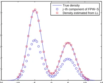
dif-ferent density estimators. The squares markers represent the density of the partition centerssj estimated by locally parametric density estima-tor: ˆf(sj) and the circle markers show the density obtained from the center’s component: ˆgj(sj)of 1-D FPW-S. . . 28 2.4 Expectations and biases of the classical PW and the 1-D FPW-S with

equally spaced partition centers. . . 28

2.5 Expectations and biases of the classical PW and the 1-D FPW-S with partition centers selected by the proposed algorithm. . . 29

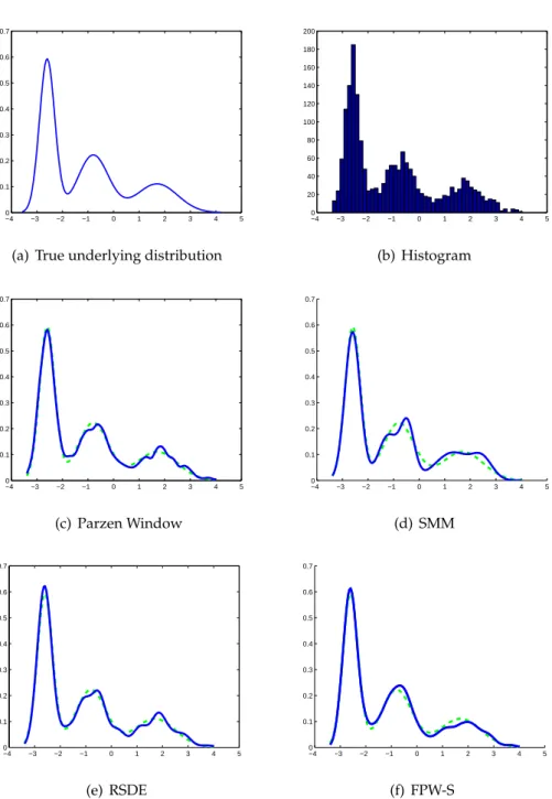
2.6 The underlying distribution and typical estimated distributions by dif-ferent approaches. Green-dashed: real density distribution; Blue: esti-mated density. . . 31

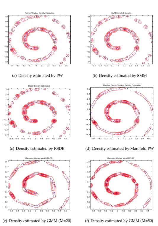
2.7 Estimated density distributions of the 2-D dataset aligned along a 1-D manifold by using different approaches: blue dots represent the data points, red contour shows the density estimated. . . 35

2.8 Estimated density distributions of the 2-D dataset aligned along a 1-D manifold by using different approaches: blue dots represent the data points, red contour shows the density estimated (continue Figure2.7). . 36

2.9 Average log-likelihood (ALL) of density models estimated by classical PW and other sparse density estimators on 22 galaxy simulation datasets. 38

2.10 Average log-likelihood (ALL) of density models estimated by classical PW and other sparse density estimators on 22 downsampled galaxy simulation datasets. . . 39

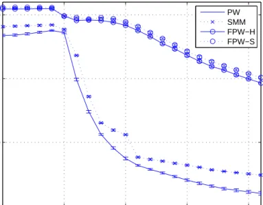
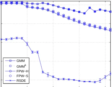
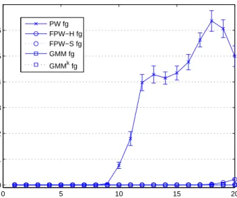
2.11 Time elapsed (in CPU seconds) on estimating the density distribution of the galaxy simulation sets by using our proposed FPW-H, FPW-S, SMM (estimated on full size simulation), GMM, GMM with K-means initialization and RSDE (estimated on downsampled simulation set). . . 40

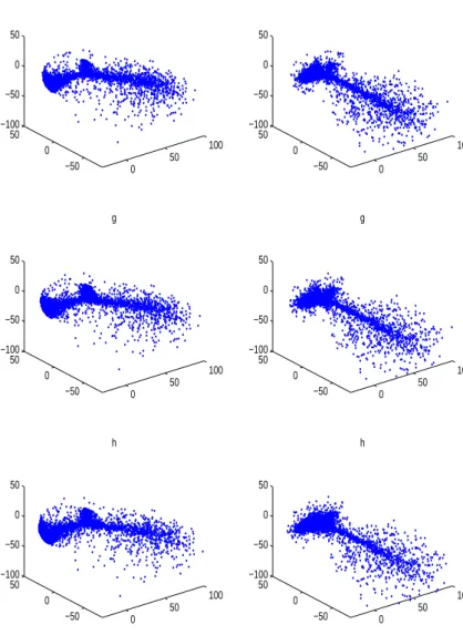
2.12 3-D projections of the simulation data for the triplet(f,g,h) = (20, 21, 22). The first projection (1st column) is onto the 3 spatial coordinates, the second (2nd column) is onto the leading 3 eigenvectors found by the Principal Component Analysis of the merged f,gandhsets. . . 41

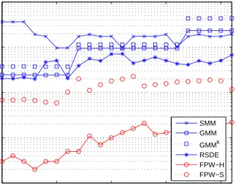
2.13 Likelihood Ratios (LR) of finding the correct source of the testing data between simulation sets f and g. . . 42

2.14 Likelihood Ratios (LR) of finding the correct source of the testing data between simulation sets g and h. . . 43

3.1 Observation space: the 2-D sky perpendicular to the line of sight is the observation plane. We use(y1,y2)to represent star’s coordinates on the

sky. The observable velocity is along the line-of-sight, which is the line connecting the observer and the star in the sky and is perpendicular to the sky. . . 47

3.2 Observation fields: observation fields are chosen according to the spa-tial distribution of the galaxy. Closed contours represent the low di-mensional structures observed and squares along with the dotted line are the chosen observational fields. . . 48

3.3 Illustration of pseudo-observation (5-PO, described later) and three sim-ulation datasets (at disruption stage 20 of disruption process F, Gand

H) on the real observation space (Mr_s), and two synthetic observation spaces (M1

3.4 Observational fields chosen for the simulation at disruption stage 20 of disruption process G. The first plot shows the spatial distribution of the simulation data, the following 3 plots illustrate the chosen observation fields and the simulation data in coordinate systemx1−x2,x2−x3and

x1−x3respectively. . . 57

3.5 Simulated observational features of fields in the vicinity of M31. . . 59

3.6 Correct rates of the proposed principled calibration on detecting the source of the pseudo-observation sets 5-POfrom triplets and 3×3 sets. . 62

3.7 Correct rates of the chi-square test and the proposed principled calibra-tion on detecting the source of the pseudo-observacalibra-tion sets 5-PO from triplets and 3×3 sets. The blue circles are the correct rates of the prin-cipled calibration and the red squares are the correct rates of the chi-square test. . . 65

4.1 Illustration of mapping from the 2-D latent space to the 3-D data space of GTM. . . 68

4.2 Learning results of GTM model with different initializations: plot (a) il-lustrates the classical initialization of GTM and the corresponding learn-ing result. Plot (b) illustrates the initialization given by our proposed manifold learning algorithm and the learning result. . . 71

4.3 Illustration of mapping from the 2-D latent space to the 3-D data space of GTM. The 2-D latent space is represented by the latent space graph. The manifold embedded in 3-D space is represented by the data space graph. . . 72

4.4 Local manifold patches associated with different types of vertices in the latent space graph. . . 76

4.5 Edges of a vertex having no parent, one parent and two parents in latent space graph. . . 76

4.6 Local manifold patches associated with the vertices in the data space graph. . . 78

4.7 Relation of the edges connected to vertices on the neighboring local manifold patches in the data space. . . 78

4.8 Plot (a) illustrates a 3-D dataset staying on a 2-D manifold. Plot (b) shows the manifold learnt by our proposed manifold expanding algo-rithm. . . 81

4.9 Illustration of the growing of the latent/data space graphs defined in our proposed manifold expanding process for learning the manifold shown in Figure4.8. . . 82

4.10 1-D manifold learnt (plot (b)) by the GTM model from 2-D dataset and its initialization (plot (a)) given by the proposed manifold learning al-gorithm. . . 84

4.11 1-D manifold learnt (plot (b)) by the GTM model from the 3-D dataset and its initialization (plot (a)) given by the proposed manifold learning algorithm. . . 85

4.12 2-D manifold learnt (plot (b)) by the GTM model from the 3-D dataset and its initialization (plot (a)) given by the proposed manifold learning algorithm. . . 85

4.13 GTM initialization, learning result, and improved result on contami-nated datasets with a different number of noise data points. (5%, 10% and 20% of each line) . . . 87

4.14 Simulation dataset at disruption stage 20: The upleft plot shows the spatial distribution. In the other 3 subplots, we view the simulation dataset in coordinate systemsx1−x2,x1−x3 andx2−x3 respectively

and use dotted rectangles to mark the regions of “stream” data points and solid rectangles to mark the regions of “shell” data points. . . 88

4.15 Manifold learnt from “stream” data points of simulations at disruption stage 15. Subplot (a) shows the original data points. The manifold sur-face learnt by our proposed algorithm is viewed from three different angles and plotted in three subplots of the second line. Subplots in the third line show the views of the improved manifold surface by GTM model. . . 90

4.16 Manifold learnt from “stream” data points of simulations at disruption stage 20. Subplot (a) shows the original data points. The manifold sur-face learnt by our proposed algorithm is viewed from three different angles and plotted in three subplots of the second line. Subplots in the third line show the views of the improved manifold surface by GTM model. . . 91

4.17 Manifold learnt from “stream” data points of simulations at disruption stage 25. Subplot (a) shows the original data points. The manifold sur-face learnt by our proposed algorithm is viewed from three different angles and plotted in three subplots of the second line. Subplots in the third line show the views of the improved manifold surface by GTM model. . . 92

4.18 Manifold learnt from “shell” data points of simulations at disruption stage 15. Subplot (a) shows the original data points. The second line show the manifold surface learnt by our proposed algorithm from dif-ferent views. . . 93

4.19 Manifold learnt from “shell” data points of simulations at disruption stage 20. Subplot (a) shows the original data points. The second line show the manifold surface learnt by our proposed algorithm from dif-ferent views. . . 94

4.20 Manifold learnt from “shell” data points of simulations at disruption stage 20. Subplot (a) shows the original data points. The second line show the manifold surface learnt by our proposed algorithm from dif-ferent views. . . 95

5.1 Multiple manifolds example: 700 3-D points aligned along a 1-D man-ifold, 2000 3-D points lying on a 2-D manifold and 600 3-D points gen-erated form a mixture of 3 Gaussians. . . 97

5.2 Tree representation of our proposed mixture model: The top level rep-resents the overall model of the whole dataset, the nodes in the second level denote the submodels of the manifolds having the same intrinsic dimensionality, each leaf in the third level corresponds to one manifold indexed bymandd. . . 101

5.3 Three intrinsic-dimension-filtered subsets of data from Figure5.1. (The value of the parameter used here is 0.0008, see Section 5.3.1.) . . . 109

5.4 Two 3-D synthetic datasets: (a) the 1-D manifold (spiral) and the 2-D manifold (S-curve) embedded are well separated. (b) the 1-D manifold (spiral) and 2-D manifold (S-curve) embedded are intersected. . . 111

5.5 The correct rates of filtering data points in the 3-D, 4-D and 10-D syn-thetic datasets into the subsets of different intrinsic dimensionalities. The x-axis represents the width of the weighting kernel used in the in-trinsic dimension estimation and the y-axis is the correct rate. . . 112

5.6 The correct rates of identifying the data points generated from the 1-D manifold (a), 2-1-D manifold (b), 3-1-D manifold (c) (in 4-1-D and 10-1-D datasets) and noise data (d) by using different parameter settings (the kernel sizer) . . . 113

5.7 Multiple manifolds aligned density model built on the 3-D dataset shown in Figure5.4(a). . . 115

5.8 Multiple manifolds aligned density model built on the 3-D dataset shown in Figure5.4(b). . . 116

5.9 Identified 2-D manifolds in a disrupted satellite galaxy at an early (a) and later (b) stages of disruption by M31. . . 117

2.1 The optimal parameters (set by 10-fold cross validation) of FPW-S for two different partition centers selecting schemes with respect to the in-creased number of the observations sampled from the distribution (2.40). 27

2.2 Error measures of density estimated by PW, SMM, RSDE and FPW-S on the 1-D dataset . . . 32

2.3 Time elapsed (in CPU seconds) on estimating and deploying the density distribution models by using PW, SMM, RSDE, FPW-S and the number of components in each density model. . . 33

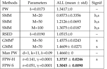
2.4 Performance measures and the parameters settings of PW, SMM, RSDE, GMMkGMM, FPW-S and FPW-H on the 1-D manifold aligned 2-D ar-tificial dataset. . . 36

2.5 Time elapsed (in CPU seconds) on estimating and deploying the density distribution models by using PW, SMM, RSDE, GMMk, GMM, FPW-S, FPW-H and the number of components in each density model. . . 37

3.1 Parameter settings for the pseudo-observation datasets. . . 60

x1, ...,xN Nobservations in the input spaceRD

Kh(·) Kernel function with smoothing parameterh ˜

f(x) Parzen window density esitmator ˆ

f(x) Estimated density function

p(x) Density distribution of the observed datax

ˆ

p(x) Fast Parzen window density esitmator L(·) Log-likelihood

K(xi,D) Knearest neighbors aroundxiin datasetD N(x;m,C) Gaussian kernel with the meanmand the

co-varianceC

δ(·) Delta function

G,Gm _{Latent space and data space graphs}

M, ˜M Projection matrix

Φ(·) Column vector with K fixed basis function

φ_j()˙

W Weight matrix of RBF network

β−1 Variance of the Gaussian distribution

U Eigenvectors matrix

U(a,b) Uniform distribution in the interval(a,b)

τ Unobserved data point in latent spaceRd

M31,M32 Galaxy names

ALL Average log likelihood

EM Expectation-Maximization algorithm

GMM Gaussian mixture models

GTM Generative Topographic Mapping

KDE Kernel density estimation

PO Pseudo-observation

PW Parzen window density esitmator

FPW Fast Parzen window density esitmator, -H: hard version, -S: soft version

RSDE Reduced Set Density Estimator

Introduction

Density estimation and dimensionality reduction are two widely discussed topics in unsupervised learning [2]. Both of them aim to discover hidden structures from the data samples without any labeled information. In density estimation, the hidden structure is represented as some stationary process from which the data samples are assumed to have been generated. The process is usually described by a probabilistic model. After estimating the parameters of the model from the current observations, the novelty of future observations could be predicted or assessed by the model. In dimensionality reduction, the hidden structure refers to a more useful and compact representation of the information in the dataset. In this case, we say that the original data points with high dimensionality actually lie along an unobserved low dimen-sional structure (i.e, manifold) embedded in the high dimendimen-sional space. It appears that density estimation and dimensionality reduction are two different problems but these can be closely related. By taking advantage of underlying manifold structure in the data, the performance of classical density estimator can be significantly improved [3]. On the other hand, by learning a probability density over the data through a latent variable model, manifolds embedded can be represented explicitly [4].

In this thesis, we estimate the density distribution of data points distributed in high dimension space but aligned along the low dimensional structures. The presented work is motivated from a joint project on studying galaxy evolutions with astronomy colleagues. There emerge two challenges from modeling the astronomical data for simulating galaxy evolutions. The first one is that the size of dataset becomesvery

large, which makes many density estimators computationally prohibitive. The second

these are non-linear in some circumstances. We address these two challenges by pre-senting sparse density estimation techniques and a novel multiple manifolds learning framework in this thesis.

In this chapter, we introduce both the classical density estimators and manifold learning algorithms. Then, we outline the thesis structure in Section 3 and highlight main contributions of the author in Section 4.

1.1

Density estimation

For a given dataset, density estimation is to construct an estimation of unobservable, underlying unknown density function based on observed data [5,6].

Parametric density estimators [7] assume a particular shape to describe the density distribution of the observed data samples. The shape is formulated by a function with parameters (e.g. unknown expectation and variance of Normal distribution), which are estimated by fitting the function to the observed dataset with optimization. For parametric density estimators, an inaccurate assumption on the density distribution will lead to an incorrect density estimation.

Semi-parametric density estimator [7] mixes a set of probability density functions from a parametric family to form a complex distribution of the data. If choosing the component as Gaussian distribution, we get a Gaussian mixture model [8]. Since the label information indicating from which component of the mixture the data points were generated is unknown, it is not straightforward to estimating the parameters of a semi-parametric density estimator (mixture model). The Expectation-Maximization (EM) [9] algorithm solves this problem by introducing an Expectation (E) step to com-pute the responsibility of the component to each data points. Then it calculates the parameters in the Maximization (M) step by maximizing the expected complete-data (including the observed data and the unobserved label information) log likelihood function using the responsibility obtained in E step.

Both parametric density and semi-parametric density estimators are based on the assumption of the density distribution of the observed data. Prior knowledge for mak-ing this kind of assumption may not be available in many cases. It might be because the density distribution is very complex itself or the data is new to the analyst that

no prior knowledge of data properties could be used. Non-parametric density esti-mations [7,10] therefore were proposed to show the structure of the distribution from the data itself like simple histogram [11, 12] nonparametric density estimator. An-other widely used non-parametric density estimator is Kernel Density Estimator, or KDE [11,13]. It provides a much smoother representation of the density distribution compared to histogram.

In Kernel Density Estimator [11,14], each observed data point is associated with a smooth kernel. The overall density is represented by the sum of these kernels. The accuracy of the kernel density estimator depends mainly on the width of the smooth kernel. With a too small value of the width, kernel density estimator gives a density distribution over-fitting to the observed data, but if the width is too large, some fine structure of the density distribution may not be captured. Variable kernel density esti-mator [11,15,16] was proposed to improve the accuracy of the classical kernel density estimator by replacing the single kernel width byNvarious values (Nis the size of the dataset). So a varied of degrees of smoothing are considered at different data points. One example of the variable kernel density estimator is manifold Parzen Windows estimator [3]. It uses Gaussians as the kernels and assumes that the high dimensional data points lie on a low dimensional structure (which is called “manifold”). Instead of using the same covariance for all the Gaussian kernels, manifold Parzen Windows es-timates the covariance of the Gaussian on top of each data point according to its local manifold patch. By employing the Gaussian kernel aligned along the manifold, the method of manifold Parzen Windows gives more weights on the data points aligned along the manifolds and demonstrates the improved estimation accuracy on high di-mensional data lying on low didi-mensional manifold.

For estimating the density distribution of a real dataset by kernel density estimator, the main concern is its computational complexity. Since all the observed data points are used to form the density distribution, the basic form of this method can be com-putationally prohibitive when the dataset is very large. This situation will get worse when dealing with dataset of high dimensionality, because kernel density estimator requires more observed data points to estimate the density distribution accurately. To reduce the computational cost in kernel density estimator, many different strategies have been presented in the past. In the case of Gaussian kernels, Fast Gauss Transform

(FGT) [17,18,19] and Improved FGT (IFGT) [20] can be used to speed up the summa-tions of Gaussians, which dominates the overall cost of kernel density estimator. For a wider range of isotropic kernels, the computational efficiency could be significantly improved by arranging the dataset in a tree-type multiresolution data structure such as Dual Tree [21] (kd-tree [22] and Anchors Hierarchy data structure). However the practical performance of these techniques (generally called N-body approach [23]) are relatively sensitive to the choices of critical hyperparameters and the dimensionality of the data [24, 25]. Another class of approaches to break down the computational complexity are reducing the amount of kernels (or components) directly in the den-sity estimation, which will be detailed in the next chapter.

1.2

Dimensionality reduction/manifold learning algorithms

xi =F(τi) +i, i∈ {1, . . . ,N}, (1.1) where we assume thatxi is sampled possibly with the noisei from the manifold F parametrized byτi ∈Rd(d<D). Bydimensionality reductionwe refer to the estimation of the low dimensional coordinatesτi’s from the observationsxi’s with a underlying relationship (1.1). Bymanifold learning, we mean the reconstruction of F(·)from the data. In general, we call these algorithms manifold learning algorithms in this thesis.

Many different approaches were proposed to find low-dimensional structures among high-dimensional data points and we can categorize them into different groups ac-cording to different classification criteria. In a simple case, we make a distinction between linear and nonlinear methods. Linear manifold learning algorithms assume that the function F(·)is a linear mapping. Examples of these algorithms are Princi-pal Components Analysis (PCA), Projection Pursuit (PP) [27,28], factor analysis (FA) [29] and classical scaling [30]. On the other hand, most of the manifold learning algo-rithms are designed to recover a non-linear relation. This kind of algoalgo-rithms include Principle curves(surface) [31], Self-organizing Mapping (SOM) [32],Generative Topo-graphic Mapping (GTM) [4], Isomap [33], LLE [34] and many more. We can also

di-vide manifold learning algorithms into convex and non-convex techniques based on the convexity of the objective function in the optimization [35].

In this work, we are particularly interested in latent variable based manifold learn-ing algorithm (e.g., GTM) because it builds an explicit probabilistic model of the em-bedding function F(·). In the probabilistic framework, the latent variable models could be easily mixed to represent more complex dataset. Accordingly, we can also represent more than one manifold in the data by mixing the generative models. In line with that, the following brief review classifies various manifold learning algo-rithms into two types: techniques without probabilistic setting and latent variable model based ones. We only introduce most common approaches here and refer read-ers to other related work.

1.2.1 Manifold learning algorithms without probabilistic setting

Principal Components Analysis (PCA) [36] is by far the most popular linear technique and it seeks a low-dimensional representation of the data by maximizing the amount of variance in the data. In mathematics, PCA can be formulated as finding the firstd

principle eigenvalues and associated eigenvectors of the covariance matrix. To cope with complex nonlinear data, some nonlinear generalizations of PCA have been devel-oped. For example, principal curves (surfaces) [31,37] attempts to provide a smooth curved approximation to data points in a least-squares sense. By employing popular kernel trick in supervised learning [38], a kernel version of PCA (KPCA) [39,40] have been derived to capture nonlinear structures embedded in high-dimensional data.

Self-organizing mapping, or SOM [32, 41] is another best-known learning algo-rithm for dimensionality reduction. It creates a set of prototype vectors representing the data set and carries out a topology preserving projection of the prototypes from the high-dimensional input space onto a low-dimensional grid. The ordered grid can be used for a convenient visualization tool for high-dimensional data [42]. For original SOM, the inter-neuron distances are not visible or measurable on the grid map such that the structures of high-dimensional data points may not be kept. To remedy the drawbacks a visualization-induced SOM (ViSOM) [43] was proposed. A comprehen-sive overview on the developments of SOM for visualization can be found in [44].

Two other nonprobabilistic methods (e.g., Locally linear embedding, or LLE [34] and Isomap [33]) for dimensionality reduction are worthy of mention as they largely

renewed research interests in developing efficient nonlinear manifold learning algo-rithms in the last few years. Basically LLE [34,45] is motivated from the assumption that each data point and its neighbors in the data should lie on or close to a locally linear patch of the manifold. It begins by computing the set of coefficients that best reconstructs each data point from its neighbors. Then LLE uses an eigenvector-based optimization technique to find the low-dimensional embedding of points while pre-serving these neighborhood coefficients. By following the same line of research of preserving local properties of the data, a number of new manifold learning algorithms were presented including Laplacian Eigenmaps [46], Hessian LLE [47], Locality pre-serving projections [48] and Local Tangent Space Alignment[26].

The Isomap algorithm [33] uses classical multidimensional scaling (MDS) [30] to recover the low dimensional representation, but seeks to preserve the intrinsic geom-etry of the data, which is captured by geodesic manifold distances between all pairs of data points. Compared to LLE, Isomap attempts to preserve geometry globally at all scales and the properties could be better understood theoretically [49]. Following the study of Isomap, some work has been recently developed to overcome the drawbacks of original algorithm [49,50,51].

1.2.2 Generative model based manifold learning algorithms

The generative model used in manifold learning is a latent variable model [52]. The representation of the distributionp(x)of the observed data in terms of latent variable is computed as: p(x) = Z p(x,τ)dτ = Z p(x|τ)p(τ)dτ (1.2) where p(x,τ)is the joint distribution and it can be decomposed into the product of the marginal distribution p(τ)of the latent variable and the conditional distribution

p(x|τ). The mapping from latent variable to data variable is represented in the condi-tional distributionp(x|τ).

One example of the linear latent variable model based manifold learning algorithm is Probabilistic Principal Component Analysis (PPCA)[53]. It assumes that the distri-bution of the latent variable is Gaussian and the mapping between the latent variable and observed variable is linear. The linear mapping is obtained from the parameter of

the data distribution p(x). It can be also viewed as a probabilistic version of classical PCA.

To model the more complex data, which aligns along a non-linear low dimensional structure, mixtures of local linear generative models such as mixture of PPCA or mix-ture of FA [54] were proposed. Although these models provide local linear mapping between local latent spaces and data spaces, the local latent spaces are not comparable with each other. i.e. the coordinate systems of neighboring components in mixture of PPCA might be differently oriented. To remedy this, the work of [55,56] proposed to learn a “global” low dimensional coordinate system for the data. Similar works were presented in [57, 58] and [59], non-linear manifold was learnt by coordinating or aligning the mixture of local linear models. Different from aligning local linear models, Generative Topographic Mapping (GTM) [4] algorithm defines in terms of a mapping from the pre-defined latent space into the data space and uses EM algorithm to optimize the mapping between the latent space and data space. Several extensions to the original GTM are reported in [60].

Among these generative model based manifold learning methods, there are a cou-ple of disadvantages: 1) The parameters are learnt from Expectation Maximization (or similar) optimization process, which is sensitive to the initialization and slow. 2) Most of the algorithms are proposed with the assumption that the datasets are generated from a single low dimensional structure, which may not be true in practice.

1.3

Thesis organization

The structure of the thesis is organized as follows:

In Chapter 1, we introduced some preliminaries for subsequent chapters: density estimation, manifold learning and probability density estimation along the underly-ing manifold. We also outlined the structure of the thesis and summarized the main contributions of the author.

Chapter 2 proposes an efficient and sparse density estimator accompanied by some theoretical analysis. First, we review the literature on the techniques of reducing the computational cost for kernel density estimators. Then we describe the proposed Fast Parzen Windows (FPW) and analyze the algorithm theoretically. The effectiveness

and efficiency of the proposed algorithm are verified on both synthetic and galaxy simulation datasets.

Chapter 3 demonstrates an application of our proposed FPW density estimation on large-scale astronomy data. After introducing the astronomical problem of calibrating galaxy disruption simulations, we present a methodology to address this problem based on the FPW density estimator. Experimental results show that FPW provides an efficient and effective way to estimate the density for large-scale astronomy datasets and the likelihood based principled calibration is much more reliable than the classical chi-square test based calibration.

Chapter 4 starts with a review of one generative model based manifold learning algorithm GTM and an illustration of the limitation of classical initialization for the parameters optimization process. Then a novel algorithm is proposed to learn the low dimensional structure, which is used to initialize the GTM model. After that, we verify our novel manifold learning algorithm on both synthetic datasets generated from non-linear manifolds and the galaxy evolution simulation dataset.

In Chapter 5, we extend the generative model for data generated from one man-ifold to a mixture model for describing the dataset generated from more than one manifold of varying dimensionality. To construct the model, we propose a multiple manifolds learning framework. The chapter finished with the demonstration of the proposed mixture model on both complex synthetic data and astronomical simula-tions data.

Chapter 6 summarizes this work and describes several future studies for future research.

1.4

Thesis contributions and publications

1. An efficient and sparse density estimator: Fast Parzen Windows (FPW) is pro-posed for large scale density estimation problems. It keeps the simplicity of the non-parametric model and avoids computationally expensive model con-struction procedures, but provides comparable performances to other density estimators on high dimensional data with low dimensional structures. Loosely

speaking, the presented FPW can be considered as a “sloppy Gaussian mixture model” (chapter2).

2. By analyzing the relation between main contributed component in FPW and the local parametric density estimator, we get some theoretical results on the perfor-mance of our proposed FPW (chapter 2).

3. A successful application of the proposed Fast Parzen Window in a density based comparison scheme for a real astronomical problem. Its efficiency of probability density estimator on large-scale dataset makes the proposed comparison scheme possible (chapter 3).

4. A new GTM initialization scheme is proposed. It captures the non-linear low dimensional structure in data space and leads to a significant improved result over classical GTM initialization (chapter 4).

5. A novel mixture model based framework is presented to learn multiple mani-folds of possibly different intrinsic dimensionalities (chapter 5).

The work resulting from these investigations has been published in a couple of papers:

Publication list

• X. Wang, P. Ti ˇno and M. A. Fardal,Multiple manifolds learning framework based on hierarchical mixture density model, In proceeding of European Conference on Machine Learning and Principles and Practice of Knowledge Discovery in Databases (ECML PKDD), 2008. (Oral presentation)

• X.Wang, P. Ti ˇno, M. A. Fardal, S. Raychaudhury and A. Babul, Fast Parzen Window Density Estimator, International joint conference on Neural Network (IJCNN) 2009. (Oral presentation)

Efficient and Sparse density

estimator (Fast Parzen Windows)

In this chapter, we address the problem of learning kernel density estimation on large-scale dataset and present an efficient and sparse density estimator: Fast Parzen Win-dows (FPW) algorithm. We start with reviewing previous work on reducing the com-putational cost for classical kernel density estimator in Section 1. Then, we describe our proposed Fast Parzen Windows. In Section 3, we investigate our efficient and sparse density estimator (FPW) theoretically. Experimental results on two synthetic data sets, as well as on data sets derived from galaxy disruption simulations are re-ported in Section 4.

2.1

Efficient kernel density estimators

Kernel density estimator (KDE) [11], also known as Parzen Windows [14], is the most popular non-parametric density estimator. It estimates the density distribution as fol-lows: ˜ f(x) = 1 N N

∑

whereNis the number of the data samples in datasetD={x1, ...,xN},Kh(·)is the ker-nel function associated with each data point,his the smoothing parameter. Although the distribution of the data samples is revealed from dataset itself, classical kernel density estimator is very computationally expensive when the sample size becomes very large. The computational efficiency can be improved by reducing the amount of kernels in the density estimators. Strategies proposed in the literature include data

reduction methods [61,62], the binned kernel density estimators [63,64] and model simplifying algorithms [65,66,67,68].

2.1.1 Data Reduction Methods

The basic idea of data reduction methods is reducing a given large data set to a small representative subset on which data analysis can be carried out. The algorithms are usually proposed independent of data analysis tasks and could be used as a pre-processing step to many machine learning problems such as classification, cluster-ing and density estimation. The simplest methods of data reduction are to draw the desired number of samples in a random way[69]. These can be easily implemented and just lead to negligible computational cost. However, a stable performance is not guaranteed because of the randomness nature in these methods. A more principled technique of data reduction is classical vector quantization methods using a set of codebook vectors which minimize the quantization error [61]. Recently, [62] intro-duced a density-based data reduction method that pruning samples in a multireso-lution manner rather than with uniform resomultireso-lution. The computational efficiency of density-based method can be further enhanced by using some entropy-based criteria [70]. The characteristic of data reduction methods is that they can be broadly used for tackling a wider range of data analysis tasks as we mentioned above. If the accuracy of density estimation is a major concern, data reduction methods might not be the first choice compared to those approaches specially designed for density estimation tasks.

2.1.2 Binned kernel density estimators

Another class of approaches to reduce the computational complexity of KDE is the binned kernel density estimator [71]. The idea is to approximate the kernel den-sity estimated in Eq. (2.1) by the density obtained over a mesh of M grid points

{b1,b2, . . . ,bM}, and binned kernel density reads:

˜ f(x|H) = 1 H M

∑

kernel density estimators reduces the number of kernels in the estimator from the number of the data pointsNto the number the grid pointsM.

The accuracy of the binned kernel density estimator is theoretically analyzed by Hall in [72], Scott and Sheather in [63]. Hall [64] also analyzed the case when associat-ing each bin center with different binnassociat-ing kernel. Instead of usassociat-ing the equally spaced grid binning, the work of [73] introduced other non-uniform binning schemes and demonstrated better results in terms of estimation accuracy.

However it is computationally prohibitive for binning in a high-dimensional input space and most algorithms along this line are only focused on univariate data.

2.1.3 Sparse kernel density estimators

In the last decade, sparse approximation techniques [74, 75, 76] have became very popular to tackle large scale machine learning problems including density estimation. If we denote the classical kernel density as

˜ f(x) = N

∑

whereπ_j = _N1 andϕ_j(x) =Kh(x−xj). The goal of sparse methods is to approximate ˜

f(x)by a simplified model ofMcomponents (M< N),

ˆ g(x) = M

∑

To obtain ˆg(x), several algorithms were proposed to estimate the mixing coefficientwi with the constraint∑_iM₌₁wi =1 and select the components{gi(x),i=1, . . . ,M}.

Girolami and He [65] proposedReduced Set Density Estimator (RSDE) to give a sparse estimator by directly minimizing the integrated squared error (ISE) between the simplified model and the true density. They showed that a direct minimization of ISE for a general kernel density estimator yields a sparse representation in the weighting coefficients.

Rather than RSDE, the method ofSimplified Mixture Model was proposed in [66]. It is based on clustering components of the complex mixture model. First, it groups the mixture components{ϕ_j}N

simplification errorεcan be upper bounded as ε= Z M

∑

∑

∑

_∑

∑

We can see that minimizing the upper bound ofε is equivalent to minimizing each component ¯ε_i. Consequently, the w_ig_i(x) can be obtained by minimizing the local error ¯εi, wigi(x) =arg min wigi(x) Z wigi(x)−

_∑

An earlier work along the same line was done by Goldberger and Roweis [67]. They use a different distance measure between ˆf and ˆgas

d(f˜, ˆg) = N

∑

where KL(·)is the Kullback-Leibler divergence [77]. The simplified density model (mixture of Gaussian) ˆgcan be obtained as

ˆ g =arg min ˆ g d( ˜ f, ˆg).

It is proved that the optimal density ˆgis a mixture of Gaussians obtained from group-ing the components of ˜finto clusters and collapsing all Gaussians within a cluster into a single Gaussian.

In [68], the relation between the model ˆg(x)and ˆf(x)is written in the regression form as follows ˆ g(x) =f˜(x) +(x) = N

∑

where(x)is the modeling error atxbetween the sparse kernel density estimator ˆg(x) and the PW density estimator ˜f(x). They construct the sparse kernel density ˆg(x)by using a forward constrained regression [78]. The algorithm selects the component

gi of the sparse kernel density estimator sequentially from the kernels formed from dataset. The learning procedure terminates when the accuracy of the sparse kernel density estimator ˆg(x)is sufficiently close to that of the PW density estimator ˜f(x).

For the algorithms discussed above, although the complex model is replaced by an optimized simple sparse one, the model construction process (i.e., evaluating ˜f(x) in (2.3)) must first be accomplished, which is still a problem for large scale dataset. In order to keep the simplicity of the nonparametric model and avoid the complex model construction procedures, we propose a new efficient and sparse density esti-mator: Fast Parzen Window density estimator to reduce the computational cost of PW. The idea is to cover the entire data space by a set of hyper-discs of fixed radii. With carefully chosen radii, the density of the partitioned disk cells can be described by a full covariance Gaussian kernel and the local data structure could be well pre-served. The global model is formed by a mixture of such locally fitted Gaussians with appropriately mixing weights.

2.2

Fast Parzen Windows density estimator

The basic idea of Fast Parzen Window (FPW) is to segment the whole data set into hyper-discs with fixed radii first. Then it fits a full covariance Gaussian kernel to the data points in each hyper-disc and updates the weights of the mixing kernels. Since we employ Gaussians as the local data-adaptive kernels [3], our density estimator reads:

ˆ p(x;r) = M

∑

N(x;mj,Cj) = 1 q (2π)D_||C j|| exp{−1 2(x−mj) T_C−1 j (x−mj)}. (2.8)

HereDis the dimension of the data point,||Cj||denotes the determinant ofCj. Note thatN(x;mj,Cj)is designed to fit the local distribution of the segment (hyper-disc)Sj.

2.2.1 Partitioning the Dataset

The first step of FPW density estimation is partitioning the data space with hyper-discs of fixed radii r, so that the data distribution could be approximated by local densities fitted within the hyper-discs. We use the following algorithm to position the hyper-discs:

1. SetS=∅(set of hyper-disc centers),ζ = ∅(set of already processed data points fromD).

2. Randomly select a data pointx ∈ Dand declare it to be the first selected center

s1,s1 =x.

• Adds1to the partition setS:S←S∪ {s1}.

• Initialize the corresponding partitionS1:S1= {x}.

• Record thatxhas been processed:ζ ←ζ∪ {x}. • Set the center counter:k =1.

3. WhileD\ζ 6=∅(there are data points inDstill to be processed), repeat: • Select a data pointx∈D\ζ and add it to the setζ (ζ ←ζ∪ {x}).

• Compute the pairwise distancesD(x,sj),sj ∈S, betweenxand the already selected centers inS.

• If for some j, D(x,sj)≤ r, wherer > 0 is a predefined threshold, assignx to the corresponding partitionSj:Sj ←Sj∪ {x}.

• IfD(x,sj)>rfor allsj ∈S, addxas a new member of the partition setS:

– Increase the center counter:k ←k+1. Setsk =x.

– Addskto the partition setS:S←S∪ {sk}.

– Initialize the corresponding partitionSk:Sk ={x}.

We thus obtain a set of partition centersS = {s1, . . . ,sM}(M ≤ N) representing the partitions{S1, . . . ,SM}of the data setD.

Note that, unlike in vector quantization, the partition elementsSi cover the same volume but are populated according to the local density of data points. Compared

with vector quantization based downsampling algorithms, relatively more data sam-ples are chosen from sparse regions by our proposed procedure.

In Figure2.1, we uses1,s2,s3ands4, four partition centers selected sequentially to

illustrate a partition example. Figure2.1(a) shows the original partitions for selected centerss1,s2,s3 ands4 by the partition algorithm proposed above. Due to the

over-lapping among the hyper-discs, very few neighboring points were left for the center

s4and they may not be able to represent the local distribution ofs4accurately. To cope

with the overlapping, we developed two strategies: hard and soft partitions. Since the hard version can be seen as a special case of the soft version, we introduce the soft one first. In the soft manner, data points are allowed to be assigned to more than one partition. The importance of the data points on representing the local distribution of the centers is evaluated by a weighting kernel (e.g. Normal kernel in Figure2.1(e)) on the centers. The partition result of the soft version of the Fast Parzen Window (FPW-S) is illustrated in Figure2.1(d). For the hard version, data points that fell in the overlap-ping regions are assigned to its nearest partition center. Figure2.1(b) illustrates the hard version partition. It can be known that the hard version is a simplified soft one by replacing the weighting kernel with a simple uniform kernel shown in Figure2.1

(c).

2.2.2 Estimation of the locally fitted components

Some kernel-based estimators use diagonal Gaussians as mixture components. How-ever, if the true density that we would like to model is actually ‘close to’ a lower di-mensional manifold embedded in high didi-mensional input space, spherical Gaussians will spread their density mass equally along all input space directions, thus giving too much probability mass to irrelevant regions of the data space. Therefore, we employ a full covariance Gaussian to model local distribution instead.

With different weighting kernels, we implement the Fast Parzen Window algo-rithm in both hard and soft versions:

00000000 00000000 00000000 00000000 00000000 00000000 00000000 00000000 00000000 00000000 00000000 00000000 00000000 00000000 00000000 11111111 11111111 11111111 11111111 11111111 11111111 11111111 11111111 11111111 11111111 11111111 11111111 11111111 11111111 11111111 00000000 00000000 00000000 00000000 00000000 00000000 00000000 00000000 00000000 00000000 00000000 00000000 00000000 00000000 00000000 11111111 11111111 11111111 11111111 11111111 11111111 11111111 11111111 11111111 11111111 11111111 11111111 11111111 11111111 11111111 00000000 00000000 00000000 00000000 00000000 00000000 00000000 00000000 00000000 00000000 00000000 00000000 00000000 00000000 00000000 11111111 11111111 11111111 11111111 11111111 11111111 11111111 11111111 11111111 11111111 11111111 11111111 11111111 11111111 11111111 S1 S2 _S3 S4

(a) Original partition from the proposed algo-rithm

S1

S2 _S3

S4

(b) Hard version partition of the effi-cient and sparse density estimator

−1 −0.5 0 0.5 1 −1 −0.5 0 0.5 1 1.5 2

(c) Simple weight Kernel

S1

S2 _S3

S4

(d) Soft version partition of the effi-cient and sparse density estimator

−5 0 5 −0.2 −0.1 0 0.1 0.2 0.3 0.4 0.5 0.6 0.7

(e) Normal weight Kernel

Figure 2.1: Illustration of the hard and soft partitioning strategies used in FPW density estimator.

In the hard partition version (FPW-H), we determine the mean and the covari-ance matrix of each Gaussian kernel using

mj = 1 |Sj|_x

∑

∑

where|Sj|denotes the size ofSj. The weights of the partition:P(Sj)for the hard version are computed as

P(Sj) = |Sj|

N . (2.11)

• Soft version:

The soft partition ofSassociates an influence weightκ_h(xi|sj)in the partitionsj to any pointxiby the neighborhood kernel:

κ_h(xi|sj) =

K_h(xi−sj)

∑N_n=1Kh(xn−sj)

. (2.12)

whereh> 0 is the kernel scale parameter. In our experiments, in order to avoid adding more parameters, we sethto be equal to the hyper-ball radiusr.

Then the weighted means and covariance matrices of the soft FPW version (FPW-S) are computed as follows (For clarity, we put derivations in Section 2.2.3):

mj = N

∑

∑

P(Sj) = ∑

N

n=1Kh(xn−sj)

∑_iM=1∑Nn=1Kh(xn−si)

. (2.15)

Even though the sums in Eqs. (2.12)-(2.14) run through all data points, in practice we only consider only a small fraction of points where the corresponding kernel values or responsibilitiesκ_h(xi|sj)are larger than some small predefined threshold value (in

our experiments 0.00001).

It should be noted that calculating theinverseof the covariance matrices (in Eq. (2.8)) may be complicated as Cj’s may be ill-conditioned. A common way to deal with this problem is to add a small isotropic (spherical) Gaussian noise of varianceγ2

in all directions, which is done by simply addingγ2to the diagonal of the covariance matrix:Cj = Cj+γ2I, whereIis an identity matrix. In our experimentsγ2=0.00001. Since the number of kernels has been reduced to the number M of the partitions, fitting each kernel to its local distribution improves the performance of the Fast Parzen Windows density estimator without increasing the time and memory costs signifi-cantly.

2.2.3 Derivation of FPW-S’s parameters

To estimate the parameters mj, Cj and P(Sj) of the j-th mixture component in the FPW-S model, we introduce a component specific local log-likelihood of j-th mixture componentLj. The sample points are weighted through kernelKh(x−sj)in the com-ponent specific local log-likelihood and it is written as:

Lj(θ) =

N

∑

i=1

K_h(xi−sj) log[P(Sj)N(x;mj,Cj)], (2.16) whereθcollects all the free parameters (means, covariances and mixture coefficients of the mixture components).

The optimal mj andCj are obtained by differentiating Lj with respect to mj, Cj and setting the derivatives to zero. We have

mj = ∑N_i=1Kh(xi−sj)xi ∑N_n=1Kh(xn−sj) = N

∑

∑

Analogously, we obtain Cj = ∑_iN=1Kh(xi−sj)(xi−mj)(xi−mj)T ∑N_q=1Kh(xq−sj) = N

∑

∑

When solving for mixing coefficientsP(Sj), the local log-likelihoodLjneed to be extended with Lagrange multiplier to ensure the mixing coefficients summing up to unity: ˜ Lj(θ) =Lj(θ) +λ M

∑

Differentiating ˜Lj w.r.t.P(S_j)and solving for the Lagrange multiplierλwe obtain

P(Sj) = ∑

N

i=1Kh(xi−sj)

∑M_q=1∑iN=1Kh(xi−sq)

. (2.20)

The mixture coefficientsP(Sj)represent the effective weight of points in the corre-sponding regions of the data space, given the smoothing kernelsKh(x−sj). The hard version of FPW, FPW-H, can be viewed as a simple efficient approximation to FPW-S.

2.3

Theoretical investigation of FPW-S

In this section, we theoretically analyze the performance of the FPW-S in univariate case by connecting it to a non-parametric density estimator ˆf(x)(locally parametric density estimator) with parametric overtones proposed in [1]. Investigation of the properties of the latter estimator shows that it has approximately the same variance as the ordinary kernel method but potentially a smaller bias. For many situations it will be seen that [1] Efˆ(x) = f(x) +1 2σ 2 Kh2b(x) +O(h4+ (Nh)−1), Varfˆ(x) = R(K)(Nh)−1f(x)−N−1f(x)2+O(h/N) (2.21)

whereEfˆ(x)andVarfˆ(x)are the expectation and the variance of the estimated density ˆ

f(x), respectively,σ_K2 = R

zK(x)dzandR(K) =R

K(z)2dz. From (2.21), the bias of the estimated ˆf(x)is written with a bias factor functionb(x)as follows:

Efˆ(x)− f(x) = 1

2σ

2

Kh2b(x) +O(h4+ (Nh)−1).

Different from the bias of classical kernel density estimator, the bias factor function

b(x)is related to f00(x), characteristics of the parametric class and the weight functions used in estimating the density.

In [1], to estimate the locally parametric density ˆf(x) for each given data x, the author defined a local kernel-smoothed likelihood function to estimate the best local parametric approximant to the true density. Around each givenx, the local log likeli-hood [79] is defined as Ln(x,θ) = Z Kh(t−x){logf(t,θ)dFN(t)− f(t,θ)dt} =1 N N

∑

whereFN is the empirical distribution function, f(·,θ)is the given parametric model with parametersθ.

In order to make the local parametric approximant ˆf(x)comparable to our FPW-S, we choose the parametric model for the local model f(t;θ)with parametersa,µandδ

f(t;a,µ,δ) = √a 2πδexp −(t−µ) 2 2δ2 )

and Gaussian as the smooth kernel with the widthh

Kh(xi−x) = 1 √ 2πhexp −(xi−x) 2 2h2 .

Then, we derive the density estimation ˆf(x)from maximizing the local likelihood and write it in terms of the Parzen Windows estimation ˜f(x)as follows:

ˆ f(x) =f˜(x)Q−1/2exp ( −1 2 ˜ f0(x) ˜ f(x) 2 Q−1h2 ) (2.23)

where ˜f(x)is the Parzen Windows estimation with kernel widthh, i.e., ˜ f(x) = 1 N N

∑

andQis learnt from the estimated varianceδas follows:

Q= δ 2 δ2_+h2 =1− h2 δ2_+h2 =1−h 2 ( ˜ f0(x) ˜ f(x) 2 − f˜ 00_(x) ˜ f(x) ) .

Furthermore, we obtain the estimated ˆf(x)as ˆ f(x) =f˜(x) s ˜ f2_(x) ˜ f2_{(x) +h}2_f˜00_(x)f˜_(x)−h2_f˜02_(x) exp −1 2 h2f˜02(x) ˜ f2_{(x) +h}2_f˜00_{(x)f˜(x)−h}2_f˜02_(x) . (2.24)

(see appendix.1for detailed derivations).

2.3.1 Theoretical analysis of 1-D FPW-S

Here we investigate the performance of our proposed FPW-S in 1-D situation. The 1-D format of (2.7) is ˆ p(x;h) = M

∑

∑

∑

∑

whereµ_jandδ2_j are the mean and the variance of the jth 1-D Gaussian distribution. Letα_j = _N1 ∑_iN=1Kh(xi−sj), we rewrite (2.25) in the following way:

ˆ p(x;h) = 1 ∑_qM=1αq M

∑

∑

Note that here we defined g(x,α_j,µ_j,δ_j) = αj ∑M_q=1αq 1 √ 2πδ_j exp ( −(x−µj) 2 2δ2 j ) .

According to (2.16), the parameters of the component g(x,αj,µj,δ_j)can be esti-mated from the 1-D formulation of the component specific local log-likelihood, i.e.

Lj(θ) = N

∑

∑

∑

In the soft version of our proposed FPW density estimator, we use the Gaussian kernel as the local smooth kernel, i.e.,

Kh(xi−sj) = 1 √ 2πhexp ( −(xi−sj) 2 2h2 ) .

Then, the parameters estimated by Eqs. (2.28)-(2.30) can be rewritten in terms of the density of the classical Parzen Windows estimator ˜f(sj)with the window widthhas follows: (see Appendix.2for derivation details):

α_j = f˜(sj), (2.31) µ_j = h 2_f˜0_(s j) ˜ f(sj) +sj, (2.32) δ2_j = h 2_f˜2_(s j) +h4f˜00(sj)f˜(sj)−h4f˜02(sj) ˜ f2_(s j) . (2.33)

the density estimated by our FPW-S on the partition centersjis the sum of the contri-bution from componentg(x;α_j,µ_j,δ_j)and other ones, i.e.

ˆ

p(sj;h) =g1(sj) +g2(sj) +. . .+gj(sj) +. . .+gM(sj).

Instead of analyzing the overall accuracy, we investigate the contribution of com-ponentgj(sj), which is believed providing the major contribution among these com-ponents. Bringing the parameters estimated by Eqs. (2.31)-(2.33) to the formulation of componentgj(sj)of the FPW-S density estimator:

gj(sj) = α_j ∑_qM=1αq 1 √ 2πδ_j exp ( −(sj−µj) 2 2δ2_j ) , (2.34)

we have the estimated component ˆgj(sj) in terms of the classical Parzen Windows estimator ˜f(x)as: ˆ gj(sj) =gˆ(sj;αj,µj,δj) =√ f˜(sj) 2π_∑qM₌₁ f˜(sq) v u u t ˜ f2_(s j) h2_f˜2_(s j) +h4f˜00(sj)f˜(sj)−h4f˜02(sj) exp ( −1 2 h2f˜02(sj) ˜ f2_(s j) +h2f˜00(sj)f˜(sj)−h2f˜0 ) . (2.35)

Let A(x) = f˜2(x) +h2f˜00(x)f˜(x)−h2f˜02(x)and x = sj, we get the comparable results between the j-th component of our FPW-S and density estimator in [1] shown in Figure2.2. ˆ gj(sj) = 1 √ 2π∑_qM=1 f˜(sq)h ˜ f(sj) s ˜ f2_(s j) A(x) exp ( −1 2 h2f˜02(sj) A(x) ) . ˆ f(sj) = f˜(sj) s ˜ f2_(s j) A(x) exp ( −1 2 h2_f˜02_(s j) A(x) ) .

Figure 2.2: Theoratical analysis results of the component ˆgj(sj) in FPW-S algorithm and the locally parametric density estimator ˆf(sj)[1].

parametric nonparametric model learnt from local log likelihood in [1] is ˆ gj(sj) = 1 √ 2πh∑M_q=1 f˜(sq) ˆ f(sj). (2.36)

If we useεrto represent (approximate) the distance between the components’ cen-ters, the relation between component ˆgj(sj)of our FPW-S and locally parametric non-parametric model ˆf(sj)shown in (2.36) could be reformulated as:

ˆ gj(sj) = εr h√2π_∑M_q=1 f˜(sq)εr ˆ f(sj) _(2.37)

Note that, the kernel widthhis equal to the fixed radiirused at the partitioning step in our algorithm. Ifr is a very small number, the number of the partitionsM will be large. This is guaranteed by the partition algorithm in Section 2.2.1. Ifris approaching 0 (when the number of data pointsNgoes to infinity),Mwill tend to infinity. In this case, the term∑_qM=1 f˜(sq)εrapproximates

R

f(x)dx, which equals to 1. Therefore, ˆ gj(sj) = ε √ 2π∑_qM=1 f˜(sq)εr ˆ f(sj) ≈√ε 2π ˆ f(sj). (2.38)

From Eq. (2.38) and (2.21), we obtain the expectation and variance the estimated com-ponent ˆgj(sj)on partition centersjas follows:

Egˆj(sj) = ε √ 2πE ˆ f(sj) Vargˆj(sj) = ε2 2πVarfˆ(sj). (2.39)

Therefore, we could claim that the expectation and variance of the componentgj(sj)of our FPW-S at the partition centersjhave similar properties to that of the locally para-metric density estimator ˆf(sj)(up to a scale which is independent of the parameter of density estimationr). The bias of the estimated component ˆgj(sj)is also sensitive to the curvature of the true density and also related to the characteristics of the kernel form and the weight functions.

2.3.2 Numerical experiments

This subsection aims to verify the theoretical findings by some numerical simulations. The datasets we used are generated from 1-D density distribution

f(x) = 6

10N(−2.6, 0.36) + 4

10N(1.7, 0.36), (2.40) whereN(µ,δ2)denotes the normal distribution with meanµand varianceδ2. In the experiments, two different ways of selecting the partition centers are employed. One is the partition algorithm proposed in Section 2.2.1. Another one is utilizing the equally spaced partition centers.

The first experiment is to confirm the relation between the number of the observa-tions N and the algorithm parameterr (h). That is with more data samples (N), the

r (orh) goes small and the number of the components M in FPW density estimator goes large. For the equally spaced partitioning scheme, we user0to represent interval of the partition centers andM0 to represent the number of the partition centers. The estimated optimal parameters (by 10-fold cross validation) with respect to different number of observations in the dataset are reported in Table2.1. It shows that

1. Analogously to classical density estimators, for both partition schemes, the size of the partition is getting smaller as the number of the observation is getting larger. At the same time, the number of partition centers must increase to ensure the coverage of the data space.

2. Our partition algorithm requires smaller number of centers than the equally spaced partitioning scheme in the density estimation.

In the second experiment, we aim to illustrate relation between the main con-tributed component (component centered on partition centersj) in FPW-S and locally parametric density, which is formulated in Eq. (refeq: grelatedf). To do this, we gen-erate 800 data points from f(x) and use 42 equally spaced centers as the partition centers. At each partition center, we estimate the densities by local parametric den-sity model and the FPW-S component centered on it. The theoretical relation between them is formulated in Eq. (2.38). In Figure 2.3, we use red square markers to repre-sent the density estimated at the fixed centers by local parametric density (denoted by LL in the figure). Accordingly, blue circles are plotted to indicate the the contribution