Contents lists available atScienceDirect
Future Generation Computer Systems
journal homepage:www.elsevier.com/locate/fgcsDynamic energy-aware scheduling for parallel task-based application
in cloud computing
Fredy Juarez
a,b,
Jorge Ejarque
a,∗,
Rosa M. Badia
a,caBarcelona Supercomputing Center (BSC), Workflows and Distributed Computing Group, Barcelona, 08034, Spain bInstituto Tecnológico Superior de Álamo Temapache, Xoyotitla, Veracruz, 92730, Mexico
cArtificial Intelligence Research Institute (IIIA), Spanish National Research Council (CSIC), Spain
h i g h l i g h t s
• Energy-aware run-time scheduler for task-based applications.
• Model for estimating the application Energy consumption.
• Methodology to automatically generate the required power consumption profile.
• Multi-heuristic resource allocation algorithm to get solutions in polynomial time.
• Energy saving/performance trade-off evaluation for different scenarios.
a r t i c l e i n f o
Article history:
Received 1 December 2015 Received in revised form 20 April 2016
Accepted 23 June 2016 Available online 5 July 2016
Keywords: Distributed computing Cloud computing Green computing Task-based applications Energy-aware scheduling Multi-heuristic resource allocation
a b s t r a c t
Green Computing is a recent trend in computer science, which tries to reduce the energy consumption and carbon footprint produced by computers on distributed platforms such as clusters, grids, and clouds. Traditional scheduling solutions attempt to minimize processing times without taking into account the energetic cost. One of the methods for reducing energy consumption is providing scheduling policies in order to allocate tasks on specific resources that impact over the processing times and energy consumption. In this paper, we propose a real-time dynamic scheduling system to execute efficiently task-based applications on distributed computing platforms in order to minimize the energy consumption. Scheduling tasks on multiprocessors is a well known NP-hard problem and optimal solution of these problems is not feasible, we present a polynomial-time algorithm that combines a set of heuristic rules and a resource allocation technique in order to get good solutions on an affordable time scale. The proposed algorithm minimizes a multi-objective function which combines the energy-consumption and execution time according to the energy-performance importance factor provided by the resource provider or user, also taking into account sequence-dependent setup times between tasks, setup times and down times for virtual machines (VM) and energy profiles for different architectures. A prototype implementation of the scheduler has been tested with different kinds of DAG generated at random as well as on real task-based COMPSs applications. We have tested the system with different size instances and importance factors, and we have evaluated which combination provides a better solution and energy savings. Moreover, we have also evaluated the introduced overhead by measuring the time for getting the scheduling solutions for a different number of tasks, kinds of DAG, and resources, concluding that our method is suitable for run-time scheduling.
©2016 Elsevier B.V. All rights reserved.
1. Introduction
Recent studies [1,2] have estimated that around 1.5%–2.0% of the total energy consumption is consumed by data centers, and this
∗Corresponding author.
E-mail address:[email protected](J. Ejarque).
energy demand is growing extremely fast due to the popularization of Internet services and distributed computing platforms such as clusters, grids, and clouds. Regarding the efficiency of data centers, studies have concluded that, in average, around 55% of the energy consumed in a data center is consumed by the computing system and the rest is consumed by the support system such as cooling, uninterrupted power supply, etc. For that reason, green cloud http://dx.doi.org/10.1016/j.future.2016.06.029
0167-739X/©2016 Elsevier B.V. All rights reserved.
© 2018. This manuscript version is made available under the CC-BY-NC-ND 4.0 license http://creativecommons.org/licenses/by-nc-nd/4.0/
computing is essential for ensuring that the future growth of cloud computing is sustainable [3].
There are several ways to reduce the energy consumed by an application when executed on a distributed platform: It includes the usage of low-power processor architectures or dynamic voltage frequency scaling (DVFS) [4], re-design of algorithms using energy-efficient patterns in compilers [5] or changing the scheduling policies for task-based applications on the available resources [6]. Traditionally, scheduling techniques have tried to minimize the total execution time of an application(makespan—
Cmax) [7] without worrying about the energy consumed. However,
there is a trade-off between energy consumed and the execution time, and sometimes increasing the performance for a faster execution implies a higher energy consumption.
The aim of our work is to offer resource providers and end-users more options for executing task-based applications in an energy conscious manner, giving the possibility of reducing energy consumption without a significant increase in total execution time or reducing the total execution time without a significant increase in energy consumption. In this paper, we present an energy-aware scheduling system for task-based applications. To decide which is the best scheduling solution according to the energy consumed, we propose a model for estimating the energy consumed by the application for a given application and a resource power consumption profile.
Since task allocation on distributed computing resources is a well known NP-hard problem in the general form [8], due to the time limitation required for run-time schedulers, the implementation of large-time optimization algorithms is not suitable. For a real time scheduler it is convenient to develop heuristic techniques for sub-optimal solutions, in order to build a scheduling algorithm that runs in polynomial-time without performing exhaustive search. Therefore, we propose the use of a multi-heuristic resource allocation (MHRA) that is essentially a faster local search algorithm for partial solutions. The algorithm is divided into two phases: the first phase combines a set of heuristic rules for ranking an eligible group of parallel tasks for a given Direct Acyclic Graph (DAG), based on the amount of data transfers, number of task predecessors or successors and execution time. The second phase combines a set of importance factors for the resource allocation algorithm that are used to determine which is the best position in the cloud for a specific task that minimizes energy (Eflow) and makespan (Cmax). The algorithm provides good
real-time scheduling solutions in an affordable time scale. The proposed scheduler has been designed to be applied to the COMP Superscalar (COMPSs) framework [9,10]. It provides an infrastructure-agnostic task-based programming model, which facilitates the development of parallel applications in distributed computing platforms. Developers can program their applications in a sequential fashion and without caring about the details of the underlying infrastructure. They just need to identify the tasks, which are the methods of the applications, to be executed in the distributed platform. At run-time, COMPSs detects data dependencies between tasks creating a DAG. Once the DAG is created, the COMPSs runtime will use the energy-aware scheduler for allocating and executing the tasks on the available computing resources in order to minimize energy or makespan.
The scheduler has been tested with different kinds of DAGs generated at random as well as on real COMPSs applications: embarrassingly parallel (EB), parallel reduction (PR), parallel increase/reduction (PIR), matrix multiplication (MT). Using three different size instances and importance factors. We have evaluated which combination of MHRA provides a better solution and energy savings and the execution time in each case, and the effect on the cloud elasticity. Moreover, we have also evaluated the introduced overhead by measuring the time for getting the
scheduling solutions for a different number of tasks, kinds of DAG, and resources, concluding that it is suitable for run-time scheduling.
The rest of the paper is organized as follows: First, Section2
presents the related work in energy-aware scheduling and Section3gives an overview of the COMPSs framework. Afterwards, Section4formulates the energy-aware scheduling problem, and the model used to estimate the application energy consumption, the profiling methodology and the multi-heuristic resource allocation algorithm are presented in Sections5–7, respectively. In Section8, we present the experiments performed to evaluate the proposed scheduler. Finally, Section9draws the conclusions and proposes guidelines for future work.
2. Related work
Traditional task scheduling algorithms for distributed platforms such as clusters, grids, and clouds, focus in minimizing the execution time [11,12] without considering energy consumption. Regarding specific work on energy-aware scheduling two main trends can be found in the literature: (1) pure scheduling software and (2) combined scheduling hardware/software. For combined scheduling, a commonly used technique is taking profit of the Dynamic Voltage Frequency Scaling (DVFS) feature which enables processors to reduce the energy consumption. By using DVFS, processors can run at different voltage, impacting on the frequency and energy consumption.
In [13] the authors present a scheduling heuristic for reducing power consumption of precedence-constrained parallel tasks in a cluster with DVFS, the model is proposed for applications that have slack time for non-critical jobs while they scale down supply voltage for reducing energy consumption and extend execution time of jobs. The model considers homogeneous nodes as processing elements (PEs) with the same processing speed and uses green SLA negotiation in order to accept a tolerable performance loss. In our work, we take into account makespan and energy consumption in a similar way, but in addition we take into account the cloud environment and setup times for creating and destroying VMs; in contrast for reduced energy consumption, we do not use DVFS, because our model minimizes energy consumption while striving to maintain application performance.
Another approach for combining DVFS in scheduling is proposed in [14]. In this case, the authors propose a scheduling algorithm in order to reduce power consumption by applying DVFS for enabling processors to run at low frequencies and low voltages. It is only applicable for those applications in which the performance is not important or can run under certain threshold frequency. The algorithm complies with the Service Level Agreement and obeys the SLA to assign resources for the job given to the consumers. The algorithm takes into account the maximumJob
(
Fmax)
and minimumJob(
Fmin)
frequencies given foreach job and the multiple serversSithat are running at maximum
Si
(
Fmax)
and minimumSi(
Fmin)
frequencies. For specific jobs, thealgorithm selects a server that runs between,
(
Fmin,
Fmax)
andguarantees the execution performance of the job while ensuring that the job does not overuse resources. In contrast, our algorithm detects parallelism at run-time by analyzing the task dependencies of a job (application) and allocates these tasks on specific VMs that have impact on the total energy and makespan.
Beloglazov et al. [6] propose an energy-aware allocation heuristic for client applications over the data center resources, considering QoS expectations. The green Cloud architecture proposed here, it is a power model that divides the energy level consumption in an idle server and running a server with the CPU utilization controlled by DVFS for different frequency and voltage utilization. This model proposes VM allocation divided in
two parts: the first part performs VM provisioning and placing the VMs on hosts like a bin packing problem with different bin sizes and prices, and the second part performs the optimization of the current VM allocation similarly to [15] the authors use a modification of the Best Fit Decreasing (MBFD) algorithm [16]. To optimize the current VM allocation first selects VMs that need to be migrated, then the chosen VMs are placed on the hosts using an MBFD algorithm. The idea is to migrate VMs according to upper and lower utilization thresholds of the hosts in order to consolidate resources.
In [17] the authors propose a cloud controller for performance-base pricing; the cloud controller is in charge of determining actions to allocate and manage the VMs, taking into account CPU frequency scaling, pricing and geo-temporal inputs such as real-time electricity prices [18] and temperature-dependent cooling [19], the problem is balancing the trade-off between energy savings and revenue loss for performing actions by scaling CPU frequency, for creating and migrate, suspend or resume VMs that have to pay a high cost in energy. The proposed controller can determine the optimal CPU frequency between energy savings and workload performance, and can reevaluate control actions at run-time when considering geo-temporal inputs, electricity prices, and temperatures. The difference with our work is that we do not only take into account the allocation of the VMs, also we take into account the energy consumption of these actions and of the data transfer in task-based applications.
However the DVFS feature is not always available in comput-ing systems, especially when nodes are shared by different appli-cation users. In those cases, we can only use traditional software for scheduling task on resources. For instance in [7], the authors pro-pose an energy-constrained provisioning for scientific workflow ensembles, focused on the provisioning of resources for scientific workflow ensembles and address the problem of meeting energy constraints along with either budget or deadline constraints. The application model is focused on workflow based applications mod-eled as a DAG and do not take into account the time for data trans-fers. The cloud resources assume that jobs do not run concurrently on VMs and offer different VM instance types with CPU, memory, and hard disk combinations, but only a single VM instance is used for simplicity. As for our work, the problem considered take into ac-count task-based applications with fine granularity, also take into account the time and energy for data transfer, VM setup, VM shut-down and our resource profiler can model VMs with different ar-chitectures, different number of CPUs and memory.
Other examples of how to perform application scheduling with multi-objective criteria can be found in [20]. The authors propose a Bi-criteria workflow task allocation and scheduling in cloud computing environments, in order to minimize the cost incurred by using a set of resources and total execution time. The bi-criteria function takes into account the time execution and data transfer. They proposed three algorithms to schedule workflows. The first algorithm focuses on the cost incurred in execution time and transfer time of the workflow. The second algorithm aims to minimize the total execution time by makespan criterion. The third algorithm is based in the Pareto solution [21] of the first and second approach. This work is similar to our work in the use of a bi-criterion objective function, but our combination is between energy consumption and total execution time and takes into account the time and energy consumption for more elements such as cores, VMs, and nodes.
A similar approach is proposed in [22], where the authors present a cost-efficient task scheduling for executing large programs in the cloud, using two heuristic strategies. The first strategy dynamically maps tasks to the most cost-efficient VMs, based on the concept of Pareto dominance. The second strategy, a complement to the first strategy, reduces the monetary costs
of non-critical tasks. This algorithm shows that we can reduce monetary costs while producing a good makespan like [17] does, but without using the DVFS technique.
Finally, in [23] the authors propose criticality-aware dynamic task scheduling on heterogeneous architectures with OmpSs [24,25]. The paper proposes scheduling policies in order to reduce the total execution time of a task represented by DAG. The algorithm takes into account the critical path (CP) and task prioritization, by keeping two ready queues, one for critical and one for non-critical tasks respectively, and insert each task in the corresponding queue according to its priority. To execute a task in a heterogeneous platform, the critical tasks in the critical queue are assigned to fast processors and critical tasks in the non-critical queue are assigned to slow processors, in order to minimize the total execution time. Compared with our work, both seek to minimize the total execution time (Makespan), but our work also takes into account the energy consumption plus the cloud infrastructure.
3. COMP Superscalar overview
COMP Superscalar (COMPSs) is a framework that provides a programming model for the development of task-based applica-tions for distributed environments and a runtime to efficiently exe-cute them on a wide range of computational infrastructures such as clusters, grids and clouds. The aim of COMPSs is to provide an easy way to develop parallel applications, while keeping the program-mers unaware of the execution environment and parallelization details. The programmers do not require prior knowledge about the underlying infrastructure, they are only required to create a se-quential application and specify which methods of the application code will be executed remotely. This selection is done by provid-ing an annotated interface where these methods are declared with some metadata about the directionality of their parameters.
3.1. Runtime
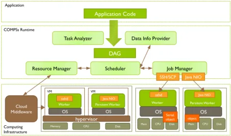
Once the application is developed with the COMPSs Program-ming Model, developers can run their task-based applications on the different distributed platforms without requiring to do any change in the code. The COMPSs runtime, shown inFig. 1, is in charge of transparently detecting the inherent parallelism and of executing the application exploiting the available resources in the distributed computing platform. To achieve this, the COMPSs run-time intercepts any method call defined as tasks and substitutes them to calls to a Task Analyzer. The Task Analyzer creates a task-dependency graph (DAG) by analyzing the data-dependencies be-tween the different invoked tasks.
Once a task is free of dependencies, the Task Scheduler is responsible of assigning a infrastructure resource to execute the task taking into account data locality, task constraints and the workload of each resource. The information required for the scheduling is provided by the Data Info provider, which tracks the locations of the different versions and replicas of the application data, and the Resource Manager, which provides the information of the available infrastructure resources and performs elasticity actions to adjust the number of resources with the current workload. When the number of tasks is higher than the available cores, the resource manager takes into account the offers of the cloud providers to determine the one that offers the resources that better fit the requirements of the application with lower economic cost. Symmetrically, when the runtime detects an excess of resources, it powers off unused instances in a cost-efficient way [26].
Finally, the Job Manager is in charge of submitting the task execution in the selected resource and of monitoring it during
Fig. 1. COMPSs runtime architecture.
its execution life-cycle. As part of this task execution monitoring, the COMPSs runtime keeps track of the duration of the different tasks executions in the different resource. With this historical data, the runtime can generate a regression model for each type of task to estimate the duration of future executions in the available resources. Once a task execution finishes, the tasks duration model is updated with the duration of the new task, the DAG is updated, possibly resulting in new dependency-free tasks that can be scheduled.
4. Problem formulation
As explained in the previous section, COMPSs translates a sequential program S into a directed acyclic graph (DAG) by evaluating data and task dependencies between parts of code in real time. The generated DAG, represented byG
=
(
T,
D)
, contains a set of vertexes T, which represents the task invocations, and a set of edgesD, which represents dependencies between task invocations. For two tasksi,
j∈
T an edge of the form(
i→
j)
denotes a relation task dependency between tasksi
,
j, where the taskjshould be executed after taskiis completed. In this senseiis called parent andjis called child. While a childjmay have many parentsi,jis only ready when all parentsihave been completed.On the other hand, a Cloud platform can be described as a set of nodes N
= {
n1,
n2, . . . ,
nm}
, where node m is represented bynm. Each nodenmis responsible for managing a set of virtual machines (VM)Vm= {
v
m1, v
m2, . . . , v
mk}
, where VMkof nodem is represented by
v
mk. Each VMv
mk has a set of processing coresCmki= {
cmk1,
cmk2, . . . ,
cmki}
, where each coreiof VMv
mk is represented bycmki.Finally, the scheduling problem consists on looking for a task schedulingS, which represents the execution order of each task jon the set of available resources. So, the scheduling for
cmki(represented bySmki) is given by the expression(1), which represents the order thatntask is executed on theith core of the
kth VM ofmth node (jn
→
cmki), and the complete scheduling solution S can be represented by expression (2), as the set of schedulings for all the resources of the Cloud.Smki
= {
j1→
cmki,
j2→
cmki, . . . ,
jn→
cmki}
(1)S
= {∀
m,k,iSmki}
.
(2)Finally, we will also refer to taskj, withj
∈
T, scheduled at coreiof VMkat nodemby the termtaskjmki, and the set of tasks scheduled atcmkiasTmkiand the set of tasks scheduled at VM
v
mkasTmk.In our scheduling problem, the process of looking for the proper task scheduling is driven by two goals:
1. To improve the energy efficiency by looking for the best positions of tasks in resources which minimize the energy consumed by the execution of the whole set of tasksT. 2. To improve the execution performance by searching for
resource allocations that minimize the total execution time. However, there is a trade-off between the optimization of the energy consumption and the total execution time. A solution which minimizes the execution time can be inefficient with regards of the energy consumption, and a solution which minimizes the energy consumption may have larger execution times. The aim of our scheduling strategy is to find a good trade-off for both problems. To achieve this goal, we propose a bi-objective cost function which combines the temporal efficiency, defined by the makespan (Cmax), and the energy efficiency, defined by the total energy
flow (Eflow) with a normalized weight factor (
α
) that indicates what is more important for the users and resource providers: the energy-efficiency or the execution time. Therefore, the proposed scheduling problem can be modeled as an optimization problem which looks for a solutionSthat minimizes the bi-objective cost function, as represented in Eq.(3).minimize
α
Eflow(
S)
Esf+
(
1−
α)
Cmax(
S)
Csf
.
(3)The cost function is composed of two main termsEflow
(
S)
andCmax
(
S)
.Eflow(
S)
is the overall energy flow which estimates the energy consumed by the execution of solutionS, andCmax(
S)
is themakespan which is defined as the maximum completion time of the latest task to leave the system [27].
To balance the bi-objective function, we apply the adaptive weighted sum method [28], which introduces a weight factor
α
, where 0≤
α
≤
1, to indicate which term is more important for the user. However, makespan and total energy flow have different units. Makespan is calculated in milliseconds, and energy is calculated in millijoules, hence, to make these metrics comparable we have introduced two factors Esf and Csf to normalize the energy consumption and execution time. As explained above, the makespan (Cmax) is basically defined by the latest task (Cn) to leave the system. However, the estimation of theEflowterm is not easy. Next section provides more details about the model used to estimateEflowfor a given schedulingS.5. Energy model
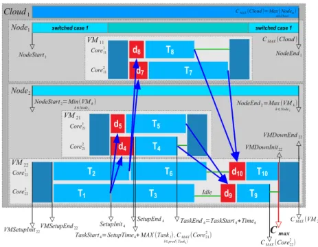
The bi-objective cost function presented in the previous section requires the calculation of the makespan (Cmax) and the overall
Fig. 2. Schedule times for all elements considered.
energy flow (Eflow) for a given a scheduling solution, such as the one described inFig. 2. From this scheduling solution, the energy-aware scheduler can extract the following application timings to estimate the total execution time and the energy consumption:
•
Start and end time of tasks’ executions in each specific core.•
Start and end time of data transfers required by each task.•
Start and end time of VMs setup and VMs shutdown.•
Start and end time of overall running time for each VM.•
Start and end time of overall running time for each node. Another key information to compute the application energy estimation, is the power profile for the different infrastructure resources. For each resource, we need to calculate the following values. The procedure to build energy profiles is explained in Section6.1. Pcmki is the proportional mean power consumed by using the
coreiof VMkin nodem.
2. Pupvmk andPdownvmk are the mean power consumed by VM when
the hypervisor creates and destroys VMkin nodem.
3. Pidlenmis the mean power consumed by a nodemin an idle state,
in other words, the power consumed when the hypervisor is not handling VMs and only the operating system services are running.
4. Pnetnm is the mean power needed for transferring data through
the cloud infrastructure.
5. PUE (Power Usage Effectiveness) is the proportional mean power consumed by the support system (UPS, cooling, etc.). With the application timings and the energy profiles we can estimate the energy consumed by each element by multiplying the duration of the different events by the corresponding mean power values. In the following paragraphs, we provide more details about how to calculate the energy consumed by the different events. First we show, how to calculate the energy consumed per task and how they are accumulated per VM and node in order to calculate the total energy flow (Eflow).
5.1. Energy consumption per task
To calculate the energy consumed by a taskjallocated on core
iof VM k in nodem (taskjmki), we have to calculate start time
(timeinitj), the setup time for transferring files (timesetupj), and the
end time (timeendj). The following paragraph describes how these
times and energy is calculated.
5.1.1. Task start time
Each taskjhas a set oflpredecessor tasks (Tprej), which must
finish before starting taskj. Therefore, the minimum starting point for task jdepending on the predecessors (timeprej) must be the
largest end time of thelpredecessor tasks which is calculated as indicated on Eq.(4), In case that taskjdoes not have predecessors, thetimeprejtime is zero.
timeprej
=
max
timeendll∈Tprej
.
(4)In the case that a taskjis the first task assigned into a core, the start time will directly set to the end time determined by the task predecessors (timeprej). However, if other tasks have already been
assigned to the same core, the start time will also depend on the end time of those tasks denoted bytimeendt. In this case, the task
start time will be determined by the maximum value between the largest predecessors end time (timeprej) and the largest end time
of previously assigned taskstat the same corecmki, expressed by max
(
timeendt)
wheret∈
Tmki. Finally, in the case thatjis the first assigned task to virtual machinekof nodem(v
mk)
, the tasks start time will also depend on the time to setup ofv
mk. If this time is larger than the largest end time of predecessor tasks, the tasks start time (timeinitj) will be equal tosetupvmk. In summary, Eq.(5)describes the way to calculate the start time of a taskj.
timeinitj
=
max
timeprej
,
max(
timeendtt∈Tmki
),
setupvmk
.
(5)5.1.2. Task setup time
Before starting the task execution, the data required by a task must be transferred to the resource which is going to execute the task. We refer to this time as setup time, which is represented by
because the amount of data to transfer will depend on the resource where predecessor taskslhave been assigned. Therefore, the setup time for taskj, described in Eq.(6), is given by the sum of all the transfer times (timetransfervmk
(
fl)
) of those required data which is out of the VM file system.timesetupj
=
l∈Tprej,l̸∈vmk
timetransfervmk
(
fl).
(6)5.1.3. Task end time
The time when a task is finished (timeendj) is easily calculated
as indicated on Eq.(7), by adding the task start time (timeinitj), the
task setup time between and the processing time of a taskjcarried out on coreiof VMkof nodem
(
timeexeccmkij
)
. This execution time is estimated by the COMPSs runtime based on historical data as introduced in Section3.1.
timeendj
=
timeinitj+
timesetupj+
timeexeccmkij.
(7)5.1.4. Task energy consumption
The energy consumption by a taskj, represented by (etaskj mki
), is estimated by the addition of the energy consumed by data file transfer and the energy consumed by the task processing. The energy consumed by file transfers is estimated by multiplying the time spent to transfer the required data by the mean power of transferring data across the network infrastructure (Pnet), while the energy consumed by task processing is estimated by multiplying the processing time of the taskjby the proportional mean power of using the assigned core in the VM (Pcmki), as indicated on Eqs.(8)
and(9)respectively.
e
transferjmk
=
timesetupj×
Pnetnm (8)e taskjmki
=
e transferjmk+
timeexeccmki j
×
Pcmki
.
(9)5.2. Energy consumption per VMs
The second set of parameters that we have to calculate to get the total energy flow is the energy consumed by each VM used in the cloud (
v
mk). This overall energy amount consumed by the virtual machine, represented byevmk, can be calculated as indicated on Eq. (10). It includes the energy consumption by setup and down of the virtual machinek of nodem, which are estimated by multiplying the time spent for setup and down of the VM (setupvmk anddownvmk) by the proportional mean power (PupvmkandPdowmvmk), and the energy consumption by the different tasksj
executed in the virtual machine
v
mkand it is calculated as shown on Eq.(11).evmk
=
setupmk×
Pupvmk+
etasksmk+
downmk×
Pdownvmk (10)etasksmk
=
i∈Cmk,j∈Tmki etaskj mki.
(11)5.3. Energy consumption per node
The energy consumed by a node (enm) is basically composed by
two terms. The first term is the aggregated energy consumption by the different VMs of a node, which can be calculated as indicated on Eq.(12).
eVm
=
vmk∈Vm
evmk
.
(12)The other term is the energy spent by the background OS services which can be estimated by a product of the time that a node is running and the mean power of a node in idle state(Pidlenm).
The calculation of the time that a node is running varies depending on the features provided by the infrastructure for powering off nodes. We have considered two scenarios:
Scenario 1: When the cloud infrastructure allows to power off nodes, the running time is determined by the duration of virtual machines running on nodem. We can calculate the node running time as indicated on Eq.(13), which is the difference between, the maximum time of the last job to be assigned to any VMs of a node (timeendj) plus the time to shutdown the corresponding VM
(downmk), and the minimum time of the first job to be assigned to any VM of a node (timeinitj) minus the time to setup of
correspond-ing VM (setupmk).
runnm
=
max(
max(
timeendjj∈vmk
)
+
downmk k∈nodem)
−
min(
min(
timeinitjj∈vmk
)
−
setupmkk∈nodem
).
(13)Scenario 2: When the cloud infrastructure does not allow to power off nodes, all nodes are running during the same time, and it corresponds to the duration of the whole application, which is also defined by the Makespan (Cmax). Therefore, the running time of a
node in this scenario can be described as in Eq.(14).
runnm
=
Cmax.
(14)Once the node running time is estimated, we can estimate the total energy consumption per node as indicated by Eq.(15)
enm
=
runnm×
Pidlenm+
eVm.
(15)5.4. Makespan and energy flow
Once we have calculated the times and partial energy consumptions for tasks, VMs and nodes, we are ready to calculate the Makespan (Cmax) and the overall energy flow (Eflow). The Makespan of the system can be calculated as shown in Eq.(16). It is basically determined by the end time of the last taskjexecuted in a cloud and the down time of the VM where this last task is executed.
Cmax
=
max(
timeendjj∈T
+
downvmk).
(16)In the case of the overall energy flow (Eflow), it can be calculated as indicated in Eq.(17)by aggregating the energy consumed by the different used node, multiplied by the proportional part of energy consumed by the data center infrastructure (cooling system, UPS,
. . .
) which is given by the Power Usage Effectiveness (PUE).Eflow
=
PUE×
nm∈N enm
.
(17) 6. Power profilingAs explained in the previous section, a power profile of the host used in the cloud is required to estimate the overall energy flow. The process of profiling consist of extracting the mean power values for the possible events of an application. In this section, we explain the methodology used to extract this power profile energy, and the values obtained for our testbed which is composed by AMD and INTEL architectures.
6.1. Power profiling procedure
The overall procedure to get the power profile is depicted in
Fig. 3. Profiling for getting power consumption by all elements.
Distribution Units (PDU) which are capable of providing the power provided to the different nodes of the Cloud. The information provided by the PDUs is aggregated by a monitoring system (Ganglia and hsflow in our case) which already provides the resource consumption (network, memory, CPU) per Node and VM. With this system we can run a set of benchmarks which stress the different parts of the system. When the benchmark process has finalized, the power usage information is extracted from Ganglia logs, and it is analyzed to make the power profiles. This power profile is automated by a set of scripts and performed in a setup phase.
The easier part of the power profile to be estimated is the mean idle powerPidlenm. In this case, we measure the mean power of the
nodes when the node is only running the background OS service (idle state), and there are no VMs and tasks or transfers running in the node.
Then, the first benchmark we can perform is the creation of a VM. In this case, for each VM template available in the system, we run a VM creation and measure the time required to create this VM
setupvmkand the mean powerPsetupvmk during the execution of this operation. A similar benchmark is performed destroying a VM and getting thedownvmktime and the mean powerPdownvmk.
A second benchmark is designed to stress cores of a VM. The main idea is to run one process per each core of VMs at the same time, starting with one process and finishing withnprocesses cor-responding with the total number of cores distributed through the VMs. Each process consumes 100% of a core. With this benchmark, we can extract the increment of power per core usedPcmki.
Finally, the last benchmark profiles the power when performing data transfers. For this benchmark, we create two VMs allocated in different nodes with one process in each VM. These processes exchange a large file between them. Measuring the mean power during the time that a VM is sending or receiving the file, we can extract the value forPnetnm. The difference observed when sending
or receiving a file is also neglectable.
We have performed the same benchmark with different VM configurations and directly to the bare metal of the host and we have measured the mean power in the different cases. Analyzing the results, we have observe different interesting facts. The first fact is that the power increment by a VM at idle is neglectable. Once the hypervisor finished with the VM creation process, the VM and Host are in an idle state. The mean power measured when running a VM at idle state is the same than the mean power with the Host at idle state. For this reason, we do not consider VM idle state in the energy model. The other important fact was observed when running the CPU stress tests. In terms of power consumption, the values obtained when running with different VM configurations were almost the same. So, as expected the power consumption depends basically on the real resource usage performed by the processes running in the VMs are doing in the physical host. Therefore, the extra power consumption introduced by the hypervisor mainly appears when a VM is created and destroyed. At operation, the overhead is just observed when
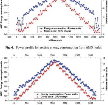
Fig. 4. Power profile for getting energy consumption from AMD nodes.
Fig. 5. Power profile for getting energy consumption from Intel nodes.
measuring the time to execute a task, and it is already taken into account when the COMPSs runtime monitors and estimates tasks duration. It means that the hypervisor does not have an observable overhead in terms mean power but it exists in terms of energy which is mainly calculated by the mean power multiplied by the execution time.
6.1.1. Testbed power profile
We have setup the profiling system and we have run the benchmarks for the different type of hosts we have in the testbed.
Figs. 4and5show the figures of the power usage for AMD and Intel nodes respectively. These figures show the relationship between the power and cores used over the time as well as the idle times.
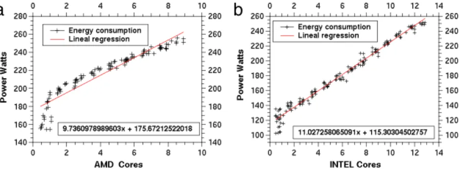
InFig. 4we can see the power in the idle state, before and after stressing cores, for an AMD host. The estimated mean power used in this case is around 175.67 W. Afterwards, when the use of cores starts, the incremental power usage is around of 9.73 W per core. The same have been done for the Intel nodes (Fig. 5), where we can observe a mean power of 115.30 W and an incremental power of 11.02 W per core used. These values have been estimated with a linear regression as shown inFig. 6.
Running the other benchmark, we can also estimate the power usage per data transfer, the transfer rate is around of 42.03 MB/s and the time and power usage for creating and destroying VMs in
Fig. 6. Linear regression to estimate the incremental power profiling.
Fig. 7. COMPSs scheduler.
Table 1
Estimated mean power consumption for the different elements of a cloud platform.
Element AMD mean power INTEL mean power
Pcmki 9.73 W 11.02 W Psetupvmk 9.49 W 18.24 W Pdownvmk 9.49 W 18.24 W Pidlenm 175.67 W 115.30 W Pnetnm 30.04 W–42.03 MB/s 27.56 W–42.03 MB/s PUE 1.2 1.2
the AMD and Intel nodes. The power profile obtained for both types of nodes is summarized inTable 1. Finally, due to the fact that both types of servers are located in the same data center the PUE will be the same.
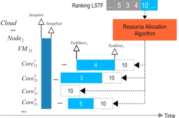
7. Multi-heuristic resource allocation
In this section, we explain a multi-heuristic resource allocation algorithm (MHRA), which generates scheduling solutions of good quality in near real-time. It is essentially a fast local search algorithm for partial solutions. MHRA builds the solution step by step, taking one task at a time and determining which is the next best location on the infrastructure.Fig. 7shows an overview of the MHRA policy. The MHRA receives as input a DAG that contains the set of tasks to be carried out on the cloud. The algorithm automatically analyzes the DAG and obtains a subset of tasks free of dependencies that can be executed in parallel. Then, for each subset, the algorithm prioritize the tasks them based on different heuristics rules and applies the resource allocation process which seeks the best resource for each task that minimizes the bi-objective cost function according to the importance factors specified by the user. This cycle between the resource allocation and the objective function evaluation is repeated for each subset of the DAG and heuristic rule. Finally, the scheduler selects the scheduling sequence generated with the heuristic rule which minimizes this cost function. This solution is sent to the COMPSs runtime to get the tasks executed following this sequence. In case that an unexpected event occurs (node failure, etc.) which
invalidates the current solution, the runtime updates the DAG and resource configuration and recalculates the scheduling repeating the same process.
The pseudo-code of MHRA algorithm is described in Algorithm 1. It can be divided into two phases:
1. The first phase applies a set of heuristic rules for ranking an eligible subset of a parallel tasks for a given DAG, based on the amount of data transfers, number of task predecessors or successors and time execution.
2. The second phase determines which is the best position (time and resource) in the cloud for each of the specific ranked tasks that minimizes energy and makespan.
7.1. Ranking initial sequences
With the objective of starting from an initial sequence of the tasks that can give a good initial solution, we first analyze the DAG in search of those tasks that do not have precedence constraints or whose tasks predecessors have already been executed. This subset of the DAG tasks can run in parallel in the cloud resources.
For this subsetT, we apply heuristic rules for ranking its tasks taking into account the characteristics of the tasks. The list shown below describe the used heuristics.
1. LPT (Longest Process Time). This rule provides greater priority to the tasks whose processing time is greater.
2. SPT (Shortest Processing Time). Selects the tasks whose processing time is smaller.
3. LNS (Longest Number of Successors). Selects the tasks that have a large number of successors.
4. LSTF (Longest Setup Times First). Selects the tasks that have a longer sequence setup time.
In Algorithm 1, lines 2 and 3 show that for each heuristic used, it applies a different energy factor of importance, lines 5 and 6 show that for each subsetTof tasks of the DAG that can run in parallel, a ranking based on each heuristics selected is used.
Fig. 8. Initial ranking and resource allocation.
7.2. Task resource allocation
After getting an initial set of sequences by applying the rules described above, we proceed to determine which is the best resource for each task. To achieve this, the resource allocation process is applied as shown in Fig. 8. It inspects the available resources and selects the best position by evaluating the objective function. The metrics used to evaluate the objective function have been described in Section5. The Algorithm 1 shows, in line 7, after ranking the subsetT, how it finds the best resource for each task
jthat will run in parallel which minimizes the objective function based on the selected heuristicsk. The cycle of line 9 tries to find a VM for the current task which improves the objective function. Line 10 builds a new solutionS′assigning to the current task a new VM and line 11 evaluates the objective function for the new solution.
Algorithm 1Multi-heuristic Resource Allocation algorithm
1: functionMHRA(DAG,Eprofile,Rcloud,Hheuristic,Fvalues) 2: for(eachk∈Hheuristic)do
3: for(eachα∈Fvalues)do
4: S= {}
5: for( eachT∈parallel(DAG))do
6: Srank=Rank(k,T) 7: for(eachtaskj∈Srank)do
8: S+ =(first(coremki∈Rcloud),taskj) 9: for(eachcoremki∈Rcloud)do
10: S′=
S+(coremki,taskj) 11: f(S′)= αEflow(S′) sf1 +(1−α) Cmax(S′) sf2 12: S′= VM_Down(S,Rcloud) 13: if(f(S′) < f(S))then
14: if(VMofcoremkiis Down )then
15: S=(VMSetupmk,timeinitj)+S′
16: end if 17: S=S′ 18: end if 19: end for 20: end for 21: end for 22: Sfactorαk =S 23: end for
24: Sheuristick=Best(Sfactorαk), withα∈Fvalues
25: end for
26: Sbest=Best(Sbestk), withk∈Hheuristic 27: return (Sbest)
28:end function
Another important aspect estimated by the algorithm is when a new VM must be created or destroyed, and the effect on time and energy consumption. In line 12 the functionVM_Dowm
()
call to algorithm 2, to determine if there are VMs that require to be switched off. The algorithm looks in all the VMs, calculating for each VM, if its downtime is greater than the time required to turn it off and turn it on, if so, it inserts into the solutionS, the VM identifier and the time in which the VM must be switchedoff. In contrast, when a resource is selected for running a task, the algorithm, in line 14, determines if a new VM is required and inserts the VM and the time in which the VM must be set up.
Algorithm 2Stop virtual machines
1:functionVM_Down(S,Rcloud) 2: Cmax=Cmax(S)
3: for(eachVMmk∈Rcloud)do 4: VMidlemk=Cmax−Cmax(VMmk) 5: if(VMidlemk>downmk+setupmk)then 6: S+ =(VMdownmk,Cmax(VMmk))
7: end if
8: end for
9: return (S) 10:end function
Finally, in lines 22–26, the best solutionS for a given initial heuristicskand
α
importance factor is assigned toSfactorαk. When all heuristics and the factors are evaluated, the solution that produces the best objective function is selected.8. Experimental evaluation
This section presents the experiments carried out to evaluate the proposed energy-aware scheduler. The first part of the section describes the configuration used for the evaluation including the machine used to run the scheduling and the cloud infrastructure, the benchmark applications and the heuristic used by the scheduler. The second part presents the results of running the energy-aware scheduling for the different benchmarks, showing the effect of the different factors and heuristics in the consumed energy, makespan, the use of resources and the cloud elasticity. The section is finalized with a set of experiments to evaluate the performance of the scheduling algorithm evaluating how the time to get the scheduling solution grows with the number of tasks and resources.
8.1. Experiments
To carry out the experiments, we have implemented a prototype of the proposed energy-aware scheduler and we have installed it in a DELL Notebook with Intel i7-2760QM CPU 2.40 GHz with 8 cores and 8 GB of memory. We have implemented several benchmarking applications with the COMPSs programming model and we have extracted the DAG generated by the runtime which is the input for the scheduler evaluation. We have simulated the scheduling solutions proposed by the energy-aware scheduler for running the applications in an private cloud infrastructure at the Barcelona Supercomputing Center (BSC).
8.1.1. Cloud infrastructure
The private cloud hosted by the BSC consist of two types of computing nodes, AMD and Intel, which are summarized inTable 2. Each node AMD contains 8 cores, a physical memory of 32 GB and a storage capacity of 800 GB, while each Intel node contains 12 cores, a physical memory of 32 GB and a storage capacity of 800 GB. For both nodes is considered a VM representative integrated of four cores, 4 GB of memory and 200 MB.
In each node AMD we can create up to 2 VMs without having a significant performance degradation. The time required to set-up the VM in these nodes is 175 s and three seconds to turn it off. For the Intel nodes we can create up to three VMs. The time required to set-up the VM is 85 s and two seconds to turn it off. The energy profile for these two types of nodes has been already presented in Section6. For the first experiments where we evaluate the effect of the different factors, we have reserved four nodes (2 AMD, 2 Intel) of this private cloud, resulting in a maximum of 10 VMs and a total of 40 cores. For the performance experiments, we have considered
Table 2
Simulation cloud infrastructure.
Element AMD node Intel node
Nodes 2–32 2–32
Physical, Memory, Storage 8, 32 GB, 800 GB 12, 32 GB, 800 GB
VMs 2 3
Cores, Memory, Storage 4, 4 GB, 200 MB 4, 4 GB, 200 MB
Setup, Down 175 s, 03 s 85 s, 02 s
Table 3
DAG size instances.
DAG size Tasks number
Small 10, 20, 30, 40, 50,60, 70, 80, 90
Medium 100, 200, 300, 400, 500, 600, 700, 800, 900
Large 1000, 2000, 3000, 4000, 5000, 6000, 7000, 8000, 9000, 10 000
Table 4
Range of values for task duration and resource consumption.
Element Range values
Process time (ms) (85 000, 1 000 000)
Number of cores (1, 4)
Physical storage (MB) (100, 1000)
Physical memory (MB) (100, 1000)
Fig. 9. DAG types MT, GT and SG of 800 tasks.
64 nodes (32 AMD, 32 Intel), resulting in a maximum of 160 VMs and a total of 640 cores.
8.1.2. Benchmark applications
As introduced before, we have implemented four benchmarking applications with the COMPSs programming model. We have executed them in the cluster and the runtime has detected the data dependencies and generated for each application a DAG of tasks. The four types of generated DAGs are enumerated below andFig. 9
depicts an example of how the different type of DAG looks like. 1. EP—Embarrassingly Parallel. Composed by n independent
parallel tasks.
2. MT—Matrix multiplication. Composed by n tasks in parallel with a chain of dependencies.
3. GT—Gather. Composed byntasks that perform a reduction with different predecessors and successors.
4. SG—Scatter–Gather. Composed by n tasks that perform an expansion and a reduction with different predecessors and successors.
For each type of DAG, we have generated three different sizes (small, medium and large) with different number of tasks as shown inTable 3. Moreover, each task has different duration, consumes a set of different resources, and has a different amount of data dependencies.Table 4shows the range of duration and resource consumption for the different DAG tasks.
8.1.3. Scheduler configuration
To generate the scheduling solutions the importance factor has to be selected, to indicate the importance of the energy versus performance and vice versa, and the heuristic rules to rank the priority of a task. The importance factor (
α
) can take any value between[
0,
1]
. For the evaluation experiments, we have selected different importance factors from 0 to 1 with intervals of 0.1.Table 5shows the relationship between the makespan (Cmax) and
energy flow (Eflow), for different importance factors.
Regarding the heuristic rules, four heuristics have been selected to classify the initial order of how the scheduler is going to allocate the tasks.
1. The LPT rule selects those tasks with longer processing time when we have a subset of parallel tasks ready to be executed. This rule tends to balance their workloads, because it is often advantageous to delay tasks with shorter processing, because these tasks will be useful at the end to balance the machines workload.
2. The SPT rule is opposite to LPT rule. It first selects those tasks with shorter process time, in order to prioritize the maximum number of executed tasks.
3. The LNS rule selects those tasks with longer number of successors. This rule is useful when the tasks are subjected to precedence constraints, aimed at ensuring that the end of the current task will fire a maximum number of parallel tasks. 4. The LSTF rule selects the task with longer sequence setup time.
This rule allows to prioritize tasks that require a longer setup time for data transfer. This situation occurs when we have a large number of predecessor tasks, where each predecessor task needs to transfer to the successor tasks its input data.
8.1.4. Experiments size
In order to take into account the size of the experimentation, the total combinations are summarized in 11 energy factors, four heuristic rules, four types of DAGs with nine small and medium runs and ten large runs as shown inTable 3, resulting a total of 4928 executions.
8.2. Impact of the importance factor in the energy/makespan trade-off
The first topic we have studied in the experimentation is the trade-off between energy and time established by the variation of the importance factor. An example of this trade-off is depicted inFig. 10. In that figure, we can see the estimated makespan and energy consumption for the solutions provided by the scheduler for a matrix multiplication (MT) DAG of 800 tasks with different importance factor and applying two different heuristic rules LSTF and LPT. For a factor 1.0 of energy, which corresponds to a factor 0.0 in makespan, we are obtaining the minimum values of energy consumption and the maximum values of the makespan for both heuristics. Subsequently, when the energy importance tends to 0.0, and the makespan factor tends to 1.0, we observe that for both the heuristic rules, the energy consumption is growing to the maximum values and the makespan is decreasing to the minimum values of the makespan.
Table 6shows the energy consumption and makespan for all combinations of importance factors
α
and the four heuristic rules for a run of MT DAG. Despite the behavior of the importance factor is similar for all of the heuristics, the values are different and depending on the DAG and resource configuration an heuristic could provide us a better solution. Moreover, we can note that the improvement in the makespan or the energy saving is associated with the heuristic used and the importance factor. So, a final user or a infrastructure provider could set the importance factor to 1 or 0 depending if it only wants to consider performance orTable 5
Energy/time importance factor—α.
Func Importance factor—α
Eflow 0.0 0.1 0.2 0.3 0.4 0.5 0.6 0.7 0.8 0.9 1.0
Cmax 1.0 0.9 0.8 0.7 0.6 0.5 0.4 0.3 0.2 0.1 0.0
Table 6
Energy consumption—Makespan per importance factor (α) and heuristic rule.
α SPT LPT LNS LSTF
Wh Cmax Wh Cmax Wh Cmax Wh Cmax
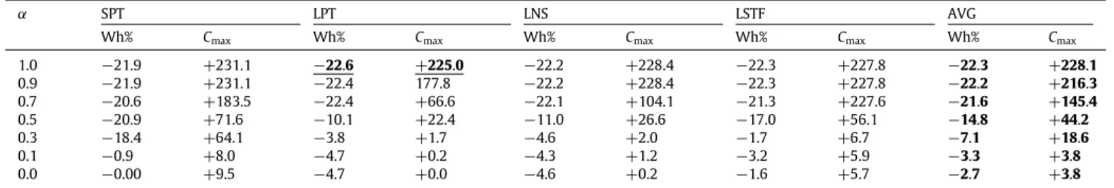
1.0 3140.3 37,834.4 3113.6 37,138.0 3128.5 37,527.4 3125.9 37,458.8 0.9 3140.3 37,834.4 3120.6 31,744.2 3128.5 37,527.4 3125.9 37,458.8 0.8 3140.3 37,834.4 3140.5 26,598.5 3181.7 24,208.1 3177.7 36,675.3 0.7 3195.7 32,390.9 3122.6 19,039.0 3133.5 23,325.6 3165.0 37,440.2 0.6 3153.1 35,640.5 3289.7 17,666.9 3132.8 19,013.9 3163.0 19,215.1 0.5 3183.3 19,607.3 3616.1 13,990.5 3578.9 14,469.8 3338.6 17,842.1 0.4 3375.4 18,399.9 3683.6 13,633.8 3755.8 13,067.8 3764.6 13,319.0 0.3 3282.1 18,753.7 3869.9 11,629.1 3837.1 11,659.3 3954.4 12,198.3 0.2 3827.4 13,701.0 3837.4 11,482.8 3811.0 11,651.2 3917.0 12,124.5 0.1 3985.7 12,349.4 3834.1 11,458.0 3848.8 11,569.1 3895.8 12,101.6 0.0 4024.8 12,521.1 3833.6 11,425.6 3838.8 11,453.3 3958.7 12,076.5 Table 7
Energy savings—Makespan degradation relationship per importance factor (α) and heuristic rule.
α SPT LPT LNS LSTF AVG
Wh% Cmax Wh% Cmax Wh% Cmax Wh% Cmax Wh% Cmax
1.0 −21.9 +231.1 −22.6 +225.0 −22.2 +228.4 −22.3 +227.8 −22.3 +228.1 0.9 −21.9 +231.1 −22.4 177.8 −22.2 +228.4 −22.3 +227.8 −22.2 +216.3 0.7 −20.6 +183.5 −22.4 +66.6 −22.1 +104.1 −21.3 +227.6 −21.6 +145.4 0.5 −20.9 +71.6 −10.1 +22.4 −11.0 +26.6 −17.0 +56.1 −14.8 +44.2 0.3 −18.4 +64.1 −3.8 +1.7 −4.6 +2.0 −1.7 +6.7 −7.1 +18.6 0.1 −0.9 +8.0 −4.7 +0.2 −4.3 +1.2 −3.2 +5.9 −3.3 +3.8 0.0 −0.00 +9.5 −4.7 +0.0 −4.6 +0.2 −1.6 +5.7 −2.7 +3.8
energy (degrading considerably the other term) or select one of the intermediate values, where he can achieve energy saving within an acceptable makespan degradation.
To illustrate it, Table 7 shows the energy savings and the makespan degradation for the different importance factor— heuristic combination. If we decide to save the maximum amount of energy in range 0
.
7≤
α
≤
1.
0, the scheduler can provide energy savings between−
21% up to−
22%, but paying a makespan increases between+
145% up to+
228%. If we decide by an average factor in range 0.
3≤
α
≤
0.
7, the energy savings average is between−
7% up to−
21% with a smaller makespan increment (+
18%). Finally, if we decide to not save energy in range 0.
0≤
α
≤
0
.
3, we could also get a small energy savings average is between−
2% up to−
7% by the selection of the correct rule, with a negligible makespan increment.8.3. Impact of the heuristic rule on the energy savings
Table 8shows the best energy savings obtained for several runs of the different DAG types (EP, MT, GT and SG) and the heuristic which has provided the best result. For instance the scheduling for a run of the EP DAG with 500 tasks achieves a reduction of
−
20.61%. The values of maximum and minimum energy consumption are 2357.54 and 1871.78 Wh and the LPT rule provides a better value than SPT, LNS, and LSTF. The energy saving is calculated as the difference between the solutions when applying the importance factor 0.0 and 1.0.In that table, we can also observe that heuristic rules are associated to instance type to solve, thus, for instances type EP and MT, we observed that the heuristic rule which gives better results is LPT. For instances type GT is LNS rule, and for instances type DG is a combination between SPT rule and LNS rule. With this observation,
we could improve the performance of our algorithm by reducing the search space by just evaluating the adequate heuristic rule according to the DAG characteristics.
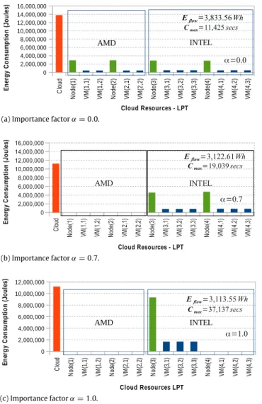
8.4. Importance factor and resource usage
Another observation we want to highlight is the relationship between the importance factor and the use of resources which is shown inFig. 11. The figure shows the number of VMs and which type of node is used for different important factors. When we have configured the scheduler without energy importance (
α
=
0.
0), it tends to use the maximum number of resources. In the case of the figure, the scheduler uses all the nodes estimating an energy consumption ofEflow=
3853.
56 Wh (equivalent to 13,800,802 J) and a makespan of Cmax=
11,
425 s. When we increase theenergy importance, the scheduler tends to prioritize the efficient nodes. In the case of
α
=
0.
7, the scheduler only uses the Intel nodes, estimating an energy consumption ofEflow=
3122.
61 Wh (equivalent to 11,241,380 J) and a makespan ofCmax=
19,
039 s.Finally, when the energy factor is the only priority (
α
=
1.
0), the trend is to use the minimum number of nodes with the lowest power consumption. In the case of the figure, the scheduler only uses one of the Intel nodes, estimating an energy consumption ofEflow
=
3113,
55 Wh inCmax=
37,
137 s which is equivalent to11,208,794 J.
This is due to the energy cost of keeping the nodes running with low load. The idle power consumption of the node is very important (it can consume up to half of the total energy), and having an unused node produces an important waste of energy.
Fig. 12shows the power consumption of the AMD and Intel nodes in an idle state and the power consumption when we use the different cores of the node. As you can see, in the figure the Intel
Table 8
Energy savings results per DAG type and heuristic rule.
T DAG type EP DAG type MT DAG type GT DAG type SG
Max Wh
Min Wh
Saving Rule Min
Wh
Max Wh
Saving Rule Min
Wh
Max Wh
Saving Rule Min
Wh Max Wh Saving Rule 100 566.98 386.71 −31.80% LPT 386.71 1054.20 −51.54% LNS 1054.20 510.85 −40.02% LNS 510.85 829.77 −46.81% SPT 200 1022.77 752.57 −26.42% LPT 752.57 1861.35 −55.27% SPT 1861.35 832.61 −34.12% SPT 832.61 1369.37 −40.44% LNS 300 1446.04 1120.09 −22.54% LPT 1120.09 2056.81 −40.88% SPT 2056.81 1215.91 −30.80% LNS 1215.91 1837.24 −34.19% SPT 400 1966.65 1511.62 −23.14% LPT 1511.62 2432.36 −35.49% SPT 2432.36 1569.23 −26.21% SPT 1569.23 2336.27 −30.97% SPT 500 2357.54 1871.68 −20.61% LPT 1871.68 2886.17 −32.09% LNS 2886.17 1959.92 −25.55% LNS 1959.92 2827.19 −29.89% LNS 600 2821.23 2242.54 −20.51% LPT 2242.54 3164.18 −25.65% LNS 3164.18 2352.46 −24.69% LNS 2352.46 3334.45 −29.35% SPT 700 3284.60 2614.56 −20.40% LPT 2614.56 3632.46 −24.76% LPT 3632.46 2732.92 −23.90% LNS 2732.92 3821.87 −26.30% LSTF 800 3785.64 3014.62 −20.37% LPT 3014.62 4024.85 −22.64% LPT 4024.85 3113.55 −22.73% LNS 3113.55 4261.20 −26.21% SPT 900 4183.82 3383.89 −19.12% LPT 3383.89 4502.43 −21.98% LPT 4502.43 3512.95 −21.47% LNS 3512.95 4750.86 −26.02% SPT 1000 4708.49 3791.76 −19.47% LPT 3791.76 4955.27 −21.36% LPT 4955.27 3897.05 −21.33% LSTF 3897.05 5284.20 −24.88% LNS
Fig. 10. Trade-off between energy and makespan.
nodes has less power usage, so this is the reason why the scheduler has prioritized the Intel nodes.
A similar behavior is observed with the VM elasticity. In this case, each VM has a cost in time (setup and down time) and its corresponding energy consumption. The MHRA algorithm will decide to use an additional VM depending on how important is the VM management cost (in time and energy) according to the objective function. To illustrate the VM, we use a SG DAG because in the scatter phase the number of parallel tasks increases, in the gather phase the number of parallel tasks is reduced.
Fig. 13shows when the scheduler decides to create and destroy a VM for the SG DAG of 800 tasks for different importance factors. In the first case (
α
=
0.
0) the energy consumption is not considered and the scheduler algorithm is looking for resource allocation to execute tasks in any VM of any node. Therefore, while the number of tasks grows, the MHRA algorithm of the scheduler starts to select new nodes and create new VMs in increasing order, using all available resources on the cloud in order to minimize the makespan. In the second case, when looking for a balance between time and energy (α
=
0.
7), the scheduler is less aggressive in the VM creation deciding to create few VMs and use it more time. This is because using less VMs, reduce the energy consumed by the hypervisor in the VM management. Moreover, using less nodes during more lime reduces the idle time, and using less resources increase the data locality and reduces the number of transfers. Finally, in the latest case (α
=
1.
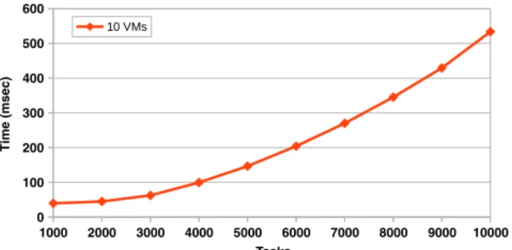
0). it only creates 3 VMs in the most energy-efficient node and uses them during all the time.8.5. Performance and overhead
To finalize the experimentation, we have analyzed the perfor-mance of the proposed scheduling system by measuring the time spent by the scheduler to get the scheduling solution (Scheduling Time) for a selected importance factor depending on the number
of tasks and resources.Fig. 14show the results of these time mea-surements. The first part of the figure shows how the time to get the scheduling solution is growing when we increase the number of tasks. In the second part of the figure, we have kept the num-ber of tasks fixed in a relatively big amount of tasks (8000 tasks) and we have measured the scheduling time increasing the number resources to consider in the scheduling problem (10–160 VMs).
To illustrate how important is this scheduling overhead, we have compare this scheduling time with application execution time (makespan). For instance, with the largest measured schedul-ing time (2717 ms.) for 8000 Tasks and 160 VMs, we can compare to the execution time of an EP DAG of this number of tasks with 10 s duration tasks which is around 130 s. It gives an overhead of 2%. Note that we have consider the time to get the best scheduling solution for the overhead evaluation. It includes the evaluate the whole graph for the different heuristics. However, the scheduling solution calculation could run in background in the runtime thread during the tasks are running. When all resource are full, the run-time remains at idle state until the end of the running tasks and can use this time to improve the solution by using backtracking techniques.
9. Conclusion and future work
In this paper, we have presented an energy-aware scheduling system for task-based applications. The scheduler aims at minimiz-ing a normalized bi-objective function which combines the energy consumption and the makespan (total execution time). Those met-rics are combined by an importance factor which enables users and service providers to indicate which is more important for their pur-poses: save energy or performance.
We have proposed a model for estimating the energy consumed by the execution of a given application in a set of resources. This model estimates the application energy consumption by
(a) Importance factorα=0.0.
(b) Importance factorα=0.7.
(c) Importance factorα=1.0.
Fig. 11. Resource usage distribution for MT DAG (800 tasks).
aggregating the consumption of the different elements of the application tasks execution, data transfers, VM management and the node background services. In addition to this model, we have proposed a methodology to automatically extract the resource power profile required to calculate the energy estimations.
The scheduler has been designed to be part of the COMP Super-scalar (COMPSs) runtime scheduler. Due to this constraint, we have proposed a Multi-heuristic Resource Allocation (MHRA) algorithm to get the best scheduling solution in polynomial time. Applica-tions in COMPSs are represented as Directed-Acyclic-Graph (DAG) of tasks dependencies which will be the input of the MHRA algo-rithm. For the different tasks graph are ranked by a set of heuristic
(a) Importance factorα=0.0.
(b) Importance factorα=0.7.
(c) Importance factorα=1.0.
Fig. 13. VM elasticity for the SG DAG (800 tasks) with different importance factors.
rules (such as SPT, LPT, LNS and LSTF) which decides the order in which the resource allocation algorithm is going to schedule them by selecting the resource which minimize the cost function.