TUTORIAL No. 1 FLUID FLOW THEORY
In order to complete this tutorial you should already have completed level 1 or have a good basic knowledge of fluid mechanics equivalent to the Engineering Council part 1 examination 103.
When you have completed this tutorial, you should be able to do the following. Explain the meaning of viscosity.
Define the units of viscosity.
Describe the basic principles of viscometers. Describe non-Newtonian flow
Explain and solve problems involving laminar flow though pipes and between parallel surfaces.
Explain and solve problems involving drag force on spheres. Explain and solve problems involving turbulent flow.
Explain and solve problems involving friction coefficient.
Throughout there are worked examples, assignments and typical exam questions. You should complete each assignment in order so that you progress from one level of knowledge to another.
1. VISCOSITY 1.1 BASIC THEORY
Molecules of fluids exert forces of attraction on each other. In liquids this is strong enough to keep the mass together but not strong enough to keep it rigid. In gases these forces are very weak and cannot hold the mass together.
When a fluid flows over a surface, the layer next to the surface may become attached to it (it wets the surface). The layers of fluid above the surface are moving so there must be shearing taking place between the layers of the fluid.
Fig.1.1
Let us suppose that the fluid is flowing over a flat surface in laminated layers from left to right as shown in figure 1.1.
y is the distance above the solid surface (no slip surface) L is an arbitrary distance from a point upstream. dy is the thickness of each layer.
dL is the length of the layer.
dx is the distance moved by each layer relative to the one below in a corresponding time dt. u is the velocity of any layer.
du is the increase in velocity between two adjacent layers.
Each layer moves a distance dx in time dt relative to the layer below it. The ratio dx/dt must be the change in velocity between layers so du = dx/dt.
When any material is deformed sideways by a (shear) force acting in the same direction, a shear stress τ is produced between the layers and a corresponding shear strain γ is produced. Shear strain is defined as follows. dy dx deformed being layer the of height n deformatio sideways = = γ
The rate of shear strain is defined as follows.
dy du dy dt dx dt taken time strain shear = γ = = = γ &
It is found that fluids such as water, oil and air, behave in such a manner that the shear stress between layers is directly proportional to the rate of shear strain.
γ =
τ constant x&
It is the constant in this formula that we know as the dynamic viscosity of the fluid. DYNAMIC VISCOSITY µ = du dy shear of rate stress shear τ = γ τ = &
FORCE BALANCE AND VELOCITY DISTRIBUTION
A shear stress τ exists between each layer and this increases by dτ over each layer. The pressure difference between the downstream end and the upstream end is dp.
The pressure change is needed to overcome the shear stress. The total force on a layer must be zero so balancing forces on one layer (assumed 1 m wide) we get the following.
dL dp dy d 0 dL d dy dp − = τ = τ +
It is normally assumed that the pressure declines uniformly with distance downstream so the pressure gradient
dL dp
is assumed constant. The minus sign indicates that the pressure falls with distance. Integrating between the no slip surface (y = 0) and any height y we get
) 1 . 1 ....( ... 2 2 dy u d dL dp dy dy du d dy d dL dp µ µ τ = − ⎟⎟ ⎠ ⎞ ⎜⎜ ⎝ ⎛ = = −
Integrating twice to solve u we get the following.
B Ay u dL dp 2 y A dy du dL dp y 2 + + µ = − + µ = −
A and B are constants of integration that should be solved based on the known conditions (boundary conditions). For the flat surface considered in figure 1.1 one boundary condition is that u = 0 when y = 0 (the no slip surface). Substitution reveals the following.
0 = 0 +0 +B hence B = 0
At some height δ above the surface, the velocity will reach the mainstream velocity uo. This gives us the second boundary condition u = uo when y = δ.
Substituting we find the following. ⎟⎟ ⎠ ⎞ ⎜⎜ ⎝ ⎛ δ + µ δ = ⎟ ⎠ ⎞ ⎜ ⎝ ⎛ δ µ − δ − + µ = − δ µ − δ − = δ + µ = δ − o o 2 o o 2 u dL dp 2 y u y u dL dp 2 u dL dp 2 y hence u dL dp 2 A A u dL dp 2
Plotting u against y gives figure 1.2.
BOUNDARY LAYER.
The velocity grows from zero at the surface to a maximum at height δ. In theory, the value of δ
is infinity but in practice it is taken as the height needed to obtain 99% of the mainstream velocity. This layer is called the boundary layer and δ is the boundary layer thickness. It is a very important concept and is discussed more fully in later work. The inverse gradient of the boundary layer is du/dy and this is the rate of shear strain γ.
1.2. UNITS of VISCOSITY 1.2.1 DYNAMIC VISCOSITY µ
The units of dynamic viscosity µ are N s/m2. It is normal in the international system (SI) to give a name to a compound unit. The old metric unit was a dyne.s/cm2 and this was called a POISE after Poiseuille. The SI unit is related to the Poise as follows.
10 Poise = 1 Ns/m2 which is not an acceptable multiple. Since, however, 1 Centi Poise (1cP) is 0.001 N s/m2 then the cP is the accepted SI unit.
1cP = 0.001 N s/m2. The symbolη is also commonly used for dynamic viscosity.
There are other ways of expressing viscosity and this is covered next. 1.2.2 KINEMATIC VISCOSITY ν
This is defined as : ν = dynamic viscosity /density ν = µ/ρ
The basic units are m2/s. The old metric unit was the cm2/s and this was called the STOKE after the British scientist. The SI unit is related to the Stoke as follows.
1 Stoke (St) = 0.0001 m2/s and is not an acceptable SI multiple. The centi Stoke (cSt),however, is 0.000001 m2/s and this is an acceptable multiple.
1cSt = 0.000001 m2/s = 1 mm2/s 1.2.3 OTHER UNITS
Other units of viscosity have come about because of the way viscosity is measured. For example REDWOOD SECONDS comes from the name of the Redwood viscometer. Other units are Engler Degrees, SAE numbers and so on. Conversion charts and formulae are available to convert them into useable engineering or SI units.
1.2.4 VISCOMETERS
The measurement of viscosity is a large and complicated subject. The principles rely on the resistance to flow or the resistance to motion through a fluid. Many of these are covered in British Standards 188. The following is a brief description of some types.
U TUBE VISCOMETER
The fluid is drawn up into a reservoir and allowed to run through a capillary tube to another reservoir in the other limb of the U tube.
The time taken for the level to fall between the marks is converted into cSt by multiplying the time by the viscometer constant.
ν = ct
The constant c should be accurately obtained by calibrating the viscometer against a master viscometer from a standards laboratory.
Fig.1.3 REDWOOD VISCOMETER
This works on the principle of allowing the fluid to run through an orifice of very accurate size in an agate block.
50 ml of fluid are allowed to fall from the level indicator into a measuring flask. The time taken is the viscosity in Redwood seconds. There are two sizes giving Redwood No.1 or No.2 seconds. These units are converted into engineering units with tables.
FALLING SPHERE VISCOMETER
This viscometer is covered in BS188 and is based on measuring the time for a small sphere to fall in a viscous fluid from one level to another. The buoyant weight of the sphere is balanced by the fluid resistance and the sphere falls with a constant velocity. The theory is based on Stokes’ Law and is only valid for very slow velocities. The theory is covered later in the section on laminar flow where it is shown that the terminal velocity (u) of the sphere is related to the dynamic viscosity (µ) and the density of the fluid and sphere (ρf and ρs) by the
formula
µ = F gd2(ρs -ρf)/18u
Fig.1.5
F is a correction factor called the Faxen correction factor, which takes into account a reduction in the velocity due to the effect of the fluid being constrained to flow between the wall of the tube and the sphere.
ROTATIONAL TYPES
There are many types of viscometers, which use the principle that it requires a torque to rotate or oscillate a disc or cylinder in a fluid. The torque is related to the viscosity. Modern instruments consist of a small electric motor, which spins a disc or cylinder in the fluid. The torsion of the connecting shaft is measured and processed into a digital readout of the viscosity in engineering units.
You should now find out more details about viscometers by reading BS188, suitable textbooks or literature from oil companies.
ASSIGNMENT No. 1
1. Describe the principle of operation of the following types of viscometers. a. Redwood Viscometers.
b. British Standard 188 glass U tube viscometer. c. British Standard 188 Falling Sphere Viscometer. d. Any form of Rotational Viscometer
2. LAMINAR FLOW THEORY
The following work only applies to Newtonian fluids. 2.1 LAMINAR FLOW
A stream line is an imaginary line with no flow normal to it, only along it. When the flow is
laminar, the streamlines are parallel and for flow between two parallel surfaces we may consider the flow as made up of parallel laminar layers. In a pipe these laminar layers are cylindrical and may be called stream tubes. In laminar flow, no mixing occurs between adjacent layers and it
occurs at low average velocities. 2.2 TURBULENT FLOW
The shearing process causes energy loss and heating of the fluid. This increases with mean velocity. When a certain critical velocity is exceeded, the streamlines break up and mixing of the fluid occurs. The diagram illustrates Reynolds coloured ribbon experiment. Coloured dye is injected into a horizontal flow. When the flow is laminar the dye passes along without mixing with the water. When the speed of the flow is increased turbulence sets in and the dye mixes with the surrounding water. One explanation of this transition is that it is necessary to change the pressure loss into other forms of energy such as angular kinetic energy as indicated by small eddies in the flow.
Fig.2.1
2.3 LAMINAR AND TURBULENT BOUNDARY LAYERS
In chapter 2 it was explained that a boundary layer is the layer in which the velocity grows
from zero at the wall (no slip surface) to 99% of the maximum and the thickness of the layer is denoted δ. When the flow within the boundary layer becomes turbulent, the shape of the boundary layers waivers and when diagrams are drawn of turbulent boundary layers, the mean shape is usually shown. Comparing a laminar and turbulent boundary layer reveals that the turbulent layer is thinner than the laminar layer.
2.4 CRITICAL VELOCITY - REYNOLDS NUMBER
When a fluid flows in a pipe at a volumetric flow rate Q m3/s the average velocity is defined A
Q
um = A is the cross sectional area. The Reynolds number is defined as
ν = µ ρ = u D u D R m m e
If you check the units of Re you will see that there are none and that it is a dimensionless number. You will learn more about such numbers in a later section.
Reynolds discovered that it was possible to predict the velocity or flow rate at which the transition from laminar to turbulent flow occurred for any Newtonian fluid in any pipe. He also discovered that the critical velocity at which it changed back again was different. He found that when the flow was gradually increased, the change from laminar to turbulent always occurred at a Reynolds number of 2500 and when the flow was gradually reduced it changed back again at a Reynolds number of 2000. Normally, 2000 is taken as the critical value.
WORKED EXAMPLE 2.1
Oil of density 860 kg/m3 has a kinematic viscosity of 40 cSt. Calculate the critical velocity when it flows in a pipe 50 mm bore diameter.
SOLUTION m/s 1.6 0.05 2000x40x10 D ν R u ν D u R 6 e m m e = = = = −
2.5 DERIVATION OF POISEUILLE'S EQUATION for LAMINAR FLOW
Poiseuille did the original derivation shown below which relates pressure loss in a pipe to the velocity and viscosity for LAMINAR FLOW. His equation is the basis for measurement of viscosity hence his name has been used for the unit of viscosity. Consider a pipe with laminar flow in it. Consider a stream tube of length ∆L at radius r and thickness dr.
Fig.2.3 y is the distance from the pipe wall.
dr du − = − = − = dy du dr dy r R y
The shear stress on the outside of the stream tube is τ. The force (Fs) acting from right
to left is due to the shear stress and is found by multiplying τ by the surface area. Fs = τ x 2πr ∆L
For a Newtonian fluid ,
dr du dy du =−µ µ =
τ . Substituting for τ we get the following.
dr du L r 2 - Fs = π ∆ µ
The pressure difference between the left end and the right end of the section is ∆p. The force due to this (Fp) is ∆p x circular area of radius r.
Fp = ∆p x πr2 rdr L 2 p du r p dr du L 2 have we forces Equating 2 ∆ ∆ − = ∆ = ∆ µ π µ πr
In order to obtain the velocity of the streamline at any radius r we must integrate between the limits u = 0 when r = R and u = u when r = r.
(
)
(
2 2)
2 2 0 L 4 p 4 L 2 p -du r R u R r L p u rdr r R u − ∆ = − ∆ ∆ − = ∆ ∆ =∫
∫
µ µ µThis is the equation of a Parabola so if the equation is plotted to show the boundary layer, it is seen to extend from zero at the edge to a maximum at the middle.
Fig.2.4 For maximum velocity put r = 0 and we get
L pR ∆ ∆ = µ 4 u1 2
The average height of a parabola is half the maximum value so the average velocity is
L pR ∆ ∆ = µ 8 u 2 m
Often we wish to calculate the pressure drop in terms of diameter D. Substitute R=D/2 and rearrange. 2 32 D Lu p= ∆ m ∆ µ
The volume flow rate is average velocity x cross sectional area.
L p D L p R L pR R Q ∆ ∆ = ∆ ∆ = ∆ ∆ = µ π µ π µ π 128 8 8 4 4 2 2 This is often changed to give the pressure drop as a friction head.
The friction head for a length L is found from hf =∆p/ρg 2 32 gD Lu hf ρ m µ =
WORKED EXAMPLE 2.2
A capillary tube is 30 mm long and 1 mm bore. The head required to produce a flow rate of 8 mm3/s is 30 mm. The fluid density is 800 kg/m3.
Calculate the dynamic and kinematic viscosity of the oil. SOLUTION
Rearranging Poiseuille's equation we get
cSt 30.11 or s / m 10 x 11 . 30 800 0241 . 0 cP 24.1 or s/m N 0241 . 0 0.01018 x 0.03 x 32 0.001 x 9.81 x 800 x 0.03 mm/s 18 . 10 785 . 0 8 A Q u mm 785 . 0 4 1 x 4 d A Lu 32 gD h 2 6 -2 m 2 2 2 m 2 f = = ρ µ = ν = = µ = = = = π = π = ρ = µ
WORKED EXAMPLE No.2.3
Oil flows in a pipe 100 mm bore with a Reynolds number of 250. The dynamic viscosity is 0.018 Ns/m2. The density is 900 kg/m3.
Determine the pressure drop per metre length, the average velocity and the radius at which it occurs. SOLUTION Re=ρum D/µ. Hence um = Re µ/ ρD um = (250 x 0.018)/(900 x 0.1) = 0.05 m/s ∆p = 32µL um /D2 ∆p = 32 x 0.018 x 1 x 0.05/0.12 ∆p= 2.88 Pascals.
u = {∆p/4Lµ}(R2 - r2) which is made equal to the average velocity 0.05 m/s 0.05 = (2.88/4 x 1 x 0.018)(0.052 - r2)
2.6. FLOW BETWEEN FLAT PLATES
Consider a small element of fluid moving at velocity u with a length dx and height dy at distance y above a flat surface. The shear stress acting on the element increases by dτ in the y direction and the pressure decreases by dp in the x direction. It was shown earlier that 2
2 dy u d dx dp µ = −
It is assumed that dp/dx does not vary with y so it may be regarded as a fixed value in the following work. Fig.2.5 ) 6 . 2 ..( ... 2 y - again g Integratin dx dp once g Integratin 2 A B Ay u dx dp A dy du y + + = + = µ µ
A and B are constants of integration. The solution of the equation now depends upon the boundary conditions that will yield A and B.
WORKED EXAMPLE No.2.4
Derive the equation linking velocity u and height y at a given point in the x direction when the flow is laminar between two stationary flat parallel plates distance h apart. Go on to derive the volume flow rate and mean velocity.
SOLUTION
When a fluid touches a surface, it sticks to it and moves with it. The velocity at the flat plates is the same as the plates and in this case is zero. The boundary conditions are hence
u = 0 when y = 0
Substituting into equation 2.6A yields that B = 0 u=0 when y=h
Substituting into equation 2.6A yields that A = (dp/dx)h/2 Putting this into equation 2.6A yields
u = (dp/dx)(1/2µ){y2 - hy}
(The student should do the algebra for this). The result is a parabolic distribution similar that given by Poiseuille's equation earlier only this time it is between two flat parallel surfaces.
FLOW RATE
To find the flow rate we consider flow through a small rectangular slit of width B and height dy at height y.
Fig.2.6
The flow through the slit is dQ = u Bdy =(dp/dx)(1/2µ){y2 - hy} Bdy Integrating between y = 0 and y = h to find Q yields
Q = -B(dp/dx)(h3/12µ)
The mean velocity is um = Q/Area = Q/Bh
hence um = -(dp/dx)(h2/12µ)
(The student should do the algebra)
2.7 CONCENTRIC CYLINDERS
This could be a shaft rotating in a bush filled with oil or a rotational viscometer. Consider a shaft rotating in a cylinder with the gap between filled with a Newtonian liquid. There is no overall flow rate so equation 2.A does not apply.
Due to the stickiness of the fluid, the liquid sticks to both surfaces and has a velocity u = ωRi at the inner
layer and zero at the outer layer.
If the gap is small, it may be assumed that the change in the velocity across the gap changes from u to zero linearly with radius r.
τ = µ du/dy
But since the change is linear du/dy = u/(Ro-Ri) = ω Ri /(Ro-Ri)
τ = µ ω Ri /(Ro-Ri) i o i i o i i R R h R Fr T R R h R h R F − = = = − = = = µω π µω π τ π 3 i 2 2 R x F Torque 2 2 area surface x stress shear F cylinder on force Shear
In the case of a rotational viscometer we rearrange so that
(
)
ω π µ h R R R T i o 3 2 − =In reality, it is unlikely that the velocity varies linearly with radius and the bottom of the cylinder would have an affect on the torque.
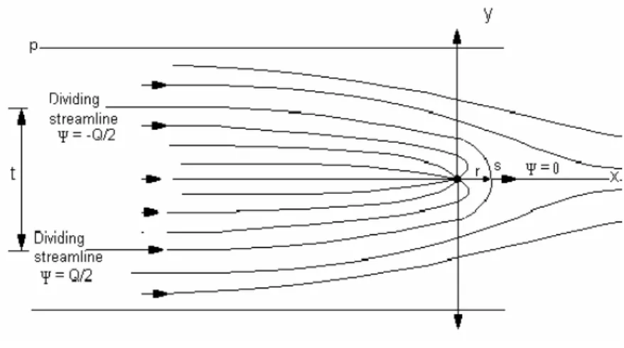
2.8 FALLING SPHERES
This theory may be applied to particle separation in tanks and to a falling sphere viscometer. When a sphere falls, it initially accelerates under the action of gravity. The resistance to motion is due to the shearing of the liquid passing around it. At some point, the resistance balances the force of gravity and the sphere falls at a constant velocity. This is the terminal velocity. For a body immersed in a liquid, the buoyant weight is W and this is equal to the viscous resistance R when the terminal velocity is reached.
R = W = volume x density difference x gravity
(
)
6 3 f s g d W R= =π ρ −ρρs = density of the sphere material
ρf = density of fluid
d = sphere diameter
The viscous resistance is much harder to derive from first principles and this will not be attempted here. In general, we use the concept of DRAG and define the DRAG COEFFICIENT as
force Resistance
2 2 2 2 d 8 4 d is sphere a of area projected The 2 is stream flow a of pressure dynamic The π ρ π ρ u R C u D =
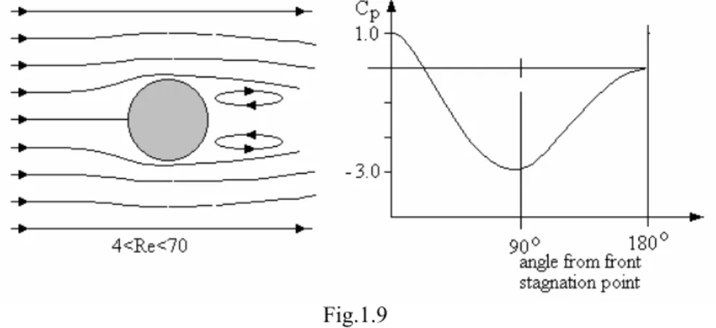
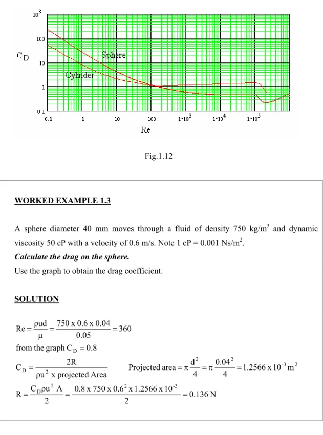
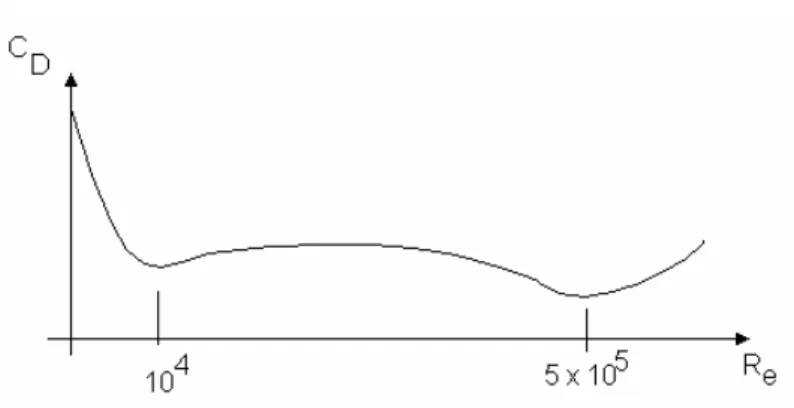
Research shows the following relationship between CD and Re for a sphere.
Fig. 2.8
For Re<0.2 the flow is called Stokes flow and Stokes showed that R = 3πdµu hence
CD=24µ/ρfud = 24/Re
For 0.2 < Re < 500 the flow is called Allen flow and CD=18.5Re-0.6
For 500 < Re < 105 CD is constant CD = 0.44
An empirical formula that covers the range 0.2 < Re < 105 is as follows.
4 . 0 1 6 24 + + + = e e D R R C
For a falling sphere viscometer, Stokes flow applies. Equating the drag force and the buoyant weight we get
3πdµu = (πd3/6)(ρs - ρf) g
µ = gd2(ρs - ρf)/18u for a falling sphere vicometer
The terminal velocity for Stokes flow is u = d2g(ρs - ρf)18µ
This formula assumes a fluid of infinite width but in a falling sphere viscometer, the liquid is squeezed between the sphere and the tube walls and additional viscous resistance is produced. The Faxen correction factor F is used to correct the result.
2.9 THRUST BEARINGS
Consider a round flat disc of radius R rotating at angular velocity ω rad/s on top of a flat surface and separated from it by an oil film of thickness t.
Fig.2.9
Assume the velocity gradient is linear in which case du/dy = u/t = ωr/t at any radius r.
32t is this D diameter of In terms 2 2 r. respect to with g integratin by found is torque total The 2 is torque The 2 is force shear The is ring on the stress shear The 4 4 R 0 3 3 2 D T t R t dr r T t dr r rdF dT t dr r dF t r dy du µπω ω µ π ω µ π ω µ π ω µ π ω µ µ τ = = = = = = = =
∫
2.10 MORE ON FLOW THROUGH PIPES
Consider an elementary thin cylindrical layer that makes an element of flow within a pipe. The length is δx , the inside radius is r and the radial thickness is dr. The pressure difference between the ends is δp and the shear stress on the surface increases by dτ from the inner to the outer surface. The velocity at any point is u and the dynamic viscosity is µ.
Fig.2.10
The pressure force acting in the direction of flow is {π(r+dr)2-πr2}δp
The shear force opposing is {(τ+δτ)(2π)(r+dr) - τ2πr}δx Equating, simplifying and ignoring the product of two small quantities we have the following result. n. integratio of constant a is A where .(A) ... 2 dr du 2 dr du r get we g Integratin dr dr du r d hence result the yields dr dr du r d ate differenti ation to differenti partial Using 1 1 so dr - dy and -y r then pipe the of inside the from measured is y If fluids. Newtonian for 2 2 2 2 2 2 2 2 2 r A x p r A x p r x p r dr u rd dr du x p r dr u rd dr du x p dr u d dr du r dr u d dr du r x p dr du dy du dr d r x p + − = + − = − = ⎟ ⎠ ⎞ ⎜ ⎝ ⎛ + ⎟ ⎠ ⎞ ⎜ ⎝ ⎛ − = + − = + − − = − = = = = + = δ δ µ δ δ µ δ δ µ δ δ µ δ δ µ µ µ δ δ µ τ µ τ τ τ δ δ
n. integratio of constant another is B where ) ...( ... ln 4 get again we g Integratin 2 B B r A x p r u=− + + δ δ µ
Equations (A) and (B) may be used to derive Poiseuille's equation or it may be used to solve flow through an annular passage.
2.10.1 PIPE
At the middle r=0 so from equation (A) it follows that A=0 At the wall, u=0 and r=R. Putting this into equation B yields
{
}
and thisisPoiseuille'sequation again. 4 1 4 4 4 0 A where ln 4 0 2 2 2 2 2 2 r R x p x p R x p r u x p R B B R A x p R − = + − = = = + + − = δ δ µ δ δ µ δ δ µ δ δ µ δ δ µ 2.10.2 ANNULUS Fig.2.11{
}
{
}
{
}
⎭ ⎬ ⎫ ⎩ ⎨ ⎧ + − = − + + − = + + − = + + − = = = = + + − = i o i i o i o i i o o R R A R R x p R R A R R x p B R A x p R C B R A x p R B r A x p r u ln 4 1 0 ln ln 4 1 0 C from D subtract ...(D) ... ... ln 4 0 ) ...( ... ... ln 4 0 . R r and R r at 0 u are conditions boundary The ln 4 2 0 2 2 2 2 2 o i 2 δ δ µ δ δ µ δ δ µ δ δ µ δ δ µ{
}
{
}
{
}
{
}
{
}
{
}
{
}
{
}
⎥ ⎥ ⎥ ⎥ ⎥ ⎦ ⎤ ⎢ ⎢ ⎢ ⎢ ⎢ ⎣ ⎡ − + ⎭ ⎬ ⎫ ⎩ ⎨ ⎧ − = ⎥ ⎥ ⎥ ⎥ ⎥ ⎦ ⎤ ⎢ ⎢ ⎢ ⎢ ⎢ ⎣ ⎡ ⎭ ⎬ ⎫ ⎩ ⎨ ⎧ − − + ⎭ ⎬ ⎫ ⎩ ⎨ ⎧ − + − = ⎥ ⎥ ⎥ ⎥ ⎥ ⎦ ⎤ ⎢ ⎢ ⎢ ⎢ ⎢ ⎣ ⎡ ⎪ ⎪ ⎭ ⎪ ⎪ ⎬ ⎫ ⎪ ⎪ ⎩ ⎪ ⎪ ⎨ ⎧ ⎭ ⎬ ⎫ ⎩ ⎨ ⎧ − − + ⎭ ⎬ ⎫ ⎩ ⎨ ⎧ − + = ⎥ ⎥ ⎥ ⎥ ⎥ ⎦ ⎤ ⎢ ⎢ ⎢ ⎢ ⎢ ⎣ ⎡ ⎪ ⎪ ⎭ ⎪ ⎪ ⎬ ⎫ ⎪ ⎪ ⎩ ⎪ ⎪ ⎨ ⎧ ⎭ ⎬ ⎫ ⎩ ⎨ ⎧ − − = + ⎭ ⎬ ⎫ ⎩ ⎨ ⎧ − + − = ⎭ ⎬ ⎫ ⎩ ⎨ ⎧ − = 2 2 2 2 2 2 2 2 2 2 2 2 2 2 2 2 2 2 2 2 2 2 2 2 ln ln 4 1 ln ln ln ln 4 1 u ln ln 4 1 ln ln 4 1 4 r -B equation into put is This ln ln 4 1 ln ln 4 1 4 0 C. from obtained be l result wil same The D. equation into back d substitute be may This ln 4 1 A r R R r R R R R x p u R R R R R R r R R R R r x p R R R R R R x p r R R R R x p x p u R R R R R R x p B B R R R R R x p x p R R R R R x p i i i o i o i i o i o i i o i o i i o i o i i o i o i i o i o i i i o i o i i o i o δ δ µ δ δ µ δ δ µ δ δ µ δ δ µ δ δ µ δ δ µ δ δ µ δ δ µFor given values the velocity distribution is similar to this.
ASSIGNMENT 2
1. Oil flows in a pipe 80 mm bore diameter with a mean velocity of 0.4 m/s. The density is 890 kg/m3 and the viscosity is 0.075 Ns/m2. Show that the flow is laminar and hence deduce the pressure loss per metre length.
(150 Pa per metre).
2. Oil flows in a pipe 100 mm bore diameter with a Reynolds’ Number of 500. The density is 800 kg/m3. Calculate the velocity of a streamline at a radius of 40 mm. The viscosity µ = 0.08 Ns/m2. (0.36 m/s)
3. A liquid of dynamic viscosity 5 x 10⁻³ Ns/m2 flows through a capillary of diameter 3.0 mm under a pressure gradient of 1800 N/m3. Evaluate the volumetric flow rate, the mean velocity, the centre line velocity and the radial position at which the velocity is equal to the mean velocity.
(uav = 0.101 m/s, umax = 0.202 m/s r = 1.06 mm) 4. Similar to Q6 1998
a. Explain the term Stokes flow and terminal velocity.
b. Show that a spherical particle with Stokes flow has a terminal velocity given by u = d2g(ρs - ρf)/18µ
Go on to show that CD=24/Re
c. For spherical particles, a useful empirical formula relating the drag coefficient and the Reynold’s number is
4 . 0 1 6 24 + + + = e e D R R C
Given ρf = 1000 kg/m3, µ= 1 cP and ρs= 2630 kg/m3 determine the maximum
size of spherical particles that will be lifted upwards by a vertical stream of water moving at 1 m/s.
d. If the water velocity is reduced to 0.5 m/s, show that particles with a diameter of less than 5.95 mm will fall downwards.
5. Similar to Q5 1998
A simple fluid coupling consists of two parallel round discs of radius R separated by a a gap h. One disc is connected to the input shaft and rotates at ω1 rad/s. The
other disc is connected to the output shaft and rotates at ω2 rad/s. The discs are
separated by oil of dynamic viscosity µ and it may be assumed that the velocity gradient is linear at all radii.
Show that the Torque at the input shaft is given by
(
)
h D T 32 2 1 4µ ω ω π − =The input shaft rotates at 900 rev/min and transmits 500W of power. Calculate the output speed, torque and power. (747 rev/min, 5.3 Nm and 414 W)
Show by application of max/min theory that the output speed is half the input speed when maximum output power is obtained.
6. Show that for fully developed laminar flow of a fluid of viscosity µ between horizontal parallel plates a distance h apart, the mean velocity um is related to the pressure gradient dp/dx by um = - (h2/12µ)(dp/dx)
Fig.2.11 shows a flanged pipe joint of internal diameter di containing viscous fluid of viscosity µ at gauge pressure p. The flange has an outer diameter do and is imperfectly tightened so that there is a narrow gap of thickness h. Obtain an expression for the leakage rate of the fluid through the flange.
Fig.2.13
Note that this is a radial flow problem and B in the notes becomes 2πr and dp/dx becomes -dp/dr. An integration between inner and outer radii will be required to give flow rate Q in terms of pressure drop p.
3. TURBULENT FLOW 3.1 FRICTION COEFFICIENT
The friction coefficient is a convenient idea that can be used to calculate the pressure drop in a pipe. It is defined as follows.
Pressure Dynamic Stress Shear Wall Cf = 3.1.1 DYNAMIC PRESSURE
Consider a fluid flowing with mean velocity um. If the kinetic energy of the fluid is converted into flow or fluid energy, the pressure would increase. The pressure rise due to this conversion is called the dynamic pressure.
KE = ½ mum2
Flow Energy = p Q Q is the volume flow rate and ρ = m/Q Equating ½ mum2 = p Q p = mu2/2Q = ½ ρ um2
3.1.2 WALL SHEAR STRESS τo
The wall shear stress is the shear stress in the layer of fluid next to the wall of the pipe.
Fig.3.1 The shear stress in the layer next to the wall is
wall o dy du ⎟⎟ ⎠ ⎞ ⎜⎜ ⎝ ⎛ =µ τ The shear force resisting flow is Fs =τoπLD The resulting pressure drop produces a force of
4 2 D p Fp π ∆ =
Equating forces gives
L p D o 4 ∆ = τ
3.1.3 FRICTION COEFFICIENT for LAMINAR FLOW 2 m f u L 4 p D 2 Pressure Dynamic Stress Shear Wall C ρ ∆ = =
From Poiseuille’s equation 2 m D Lu 32 p= µ ∆ Hence e 2 m 2 2 m f R 16 D u 16 D Lu 32 u L 4 D 2 C = ρ µ = ⎟ ⎠ ⎞ ⎜ ⎝ ⎛ µ ⎟⎟ ⎠ ⎞ ⎜⎜ ⎝ ⎛ ρ = 3.1.4 DARCY FORMULA
This formula is mainly used for calculating the pressure loss in a pipe due to turbulent flow but it can be used for laminar flow also.
Turbulent flow in pipes occurs when the Reynolds Number exceeds 2500 but this is not a clear point so 3000 is used to be sure. In order to calculate the frictional losses we use the concept of friction coefficient symbol Cf. This was defined as follows.
2 m f u L 4 p D 2 Pressure Dynamic Stress Shear Wall C ρ ∆ = =
Rearranging equation to make ∆p the subject D 2 u L C 4 p 2 m f ρ = ∆
This is often expressed as a friction head hf gD 2 Lu C 4 g p h 2 m f f ρ = ∆ =
This is the Darcy formula. In the case of laminar flow, Darcy's and Poiseuille's equations must give the same result so equating them gives
e m f 2 m 2 m f R 16 D u 16 C gD Lu 32 gD 2 Lu C 4 = ρ µ = ρ µ =
This is the same result as before for laminar flow.
Turbulent flow may be safely assumed in pipes when the Reynolds’ Number exceeds 3000. In order to calculate the frictional losses we use the concept of friction coefficient symbol Cf. Note that in older textbooks Cf was written as f but now the symbol f
represents 4Cf.
3.1.5 FLUID RESISTANCE
Fluid resistance is an alternative approach to solving problems involving losses. The above equations may be expressed in terms of flow rate Q by substituting u = Q/A
2 2 f 2 m f f gDA 2 LQ C 4 gD 2 Lu C 4
h = = Substituting A =πD2/4 we get the following.
2 5 2 2 f f RQ D g LQ C 32 h = π
= R is the fluid resistance or restriction. 322 5
D g L C R f π =
If we want pressure loss instead of head loss the equations are as follows. 2 5 2 2 f f f RQ D LQ C 32 gh p = π ρ = ρ
= R is the fluid resistance or restriction. 322 5
D L C R f π ρ =
It should be noted that R contains the friction coefficient and this is a variable with velocity and surface roughness so R should be used with care.
3.2 MOODY DIAGRAM AND RELATIVE SURFACE ROUGHNESS
In general the friction head is some function of um such that hf = φumn. Clearly for laminar flow, n =1 but for turbulent flow n is between 1 and 2 and its precise value depends upon the roughness of the pipe surface. Surface roughness promotes turbulence and the effect is shown in the following work.
Relative surface roughness is defined as ε = k/D where k is the mean surface roughness and D
the bore diameter.
An American Engineer called Moody conducted exhaustive experiments and came up with the Moody Chart. The chart is a plot of Cf vertically against Re horizontally for various values of ε. In order to use this chart you must know two of the three co-ordinates in order to pick out the point on the chart and hence pick out the unknown third co-ordinate. For smooth pipes, (the bottom curve on the diagram), various formulae have been derived such as those by Blasius and Lee.
BLASIUS Cf = 0.0791 Re0.25
LEE Cf = 0.0018 + 0.152 Re0.35.
The Moody diagram shows that the friction coefficient reduces with Reynolds number but at a certain point, it becomes constant. When this point is reached, the flow is said to be fully developed turbulent flow. This point occurs at lower Reynolds numbers for rough pipes.
A formula that gives an approximate answer for any surface roughness is that given by Haaland.
⎪⎭ ⎪ ⎬ ⎫ ⎪⎩ ⎪ ⎨ ⎧ ⎟ ⎠ ⎞ ⎜ ⎝ ⎛ ε + − = 11 . 1 e 10 f R 3.71 9 . 6 log 6 . 3 C 1
© D.J.DUNN
26
WORKED EXAMPLE 3.1
Determine the friction coefficient for a pipe 100 mm bore with a mean surface roughness of 0.06 mm when a fluid flows through it with a Reynolds number of 20 000.
SOLUTION
The mean surface roughness ε = k/d = 0.06/100 = 0.0006 Locate the line for ε = k/d = 0.0006.
Trace the line until it meets the vertical line at Re = 20 000. Read of the value of Cf horizontally on the left. Answer Cf = 0.0067.Check using the formula from Haaland.
0067 . 0 C 206 . 12 C 1 71 . 3 0006 . 0 20000 9 . 6 log 6 . 3 C 1 71 . 3 0006 . 0 20000 9 . 6 log 6 . 3 C 1 71 . 3 R 9 . 6 log 6 . 3 C 1 f f 11 . 1 10 f 11 . 1 10 f 11 . 1 e 10 f = = ⎪⎭ ⎪ ⎬ ⎫ ⎪⎩ ⎪ ⎨ ⎧ ⎟ ⎠ ⎞ ⎜ ⎝ ⎛ + − = ⎪⎭ ⎪ ⎬ ⎫ ⎪⎩ ⎪ ⎨ ⎧ ⎟ ⎠ ⎞ ⎜ ⎝ ⎛ + − = ⎪⎭ ⎪ ⎬ ⎫ ⎪⎩ ⎪ ⎨ ⎧ ⎟ ⎠ ⎞ ⎜ ⎝ ⎛ ε + − = WORKED EXAMPLE 3.2
Oil flows in a pipe 80 mm bore with a mean velocity of 4 m/s. The mean surface roughness is 0.02 mm and the length is 60 m. The dynamic viscosity is 0.005 N s/m2 and the density is 900 kg/m3. Determine the pressure loss.
SOLUTION
Re = ρud/µ = (900 x 4 x 0.08)/0.005 = 57600
ε= k/d = 0.02/80 = 0.00025 From the chart Cf = 0.0052
hf = 4CfLu2/2dg = (4 x 0.0052 x 60 x 42)/(2 x 9.81 x 0.08) = 12.72 m
ASSIGNMENT 3
1. A pipe is 25 km long and 80 mm bore diameter. The mean surface roughness is 0.03 mm. It carries oil of density 825 kg/m3 at a rate of 10 kg/s. The dynamic viscosity is 0.025 N s/m2.
Determine the friction coefficient using the Moody Chart and calculate the friction head. (Ans. 3075 m.)
2. Water flows in a pipe at 0.015 m3/s. The pipe is 50 mm bore diameter. The pressure drop is 13 420 Pa per metre length. The density is 1000 kg/m3 and the dynamic viscosity is 0.001 N s/m2.
Determine
i. the wall shear stress (167.75 Pa) ii. the dynamic pressure (29180 Pa). iii. the friction coefficient (0.00575) iv. the mean surface roughness (0.0875 mm)
3. Explain briefly what is meant by fully developed laminar flow. The velocity u at any radius r in fully developed laminar flow through a straight horizontal pipe of internal radius ro is given by
u = (1/4µ)(ro2 - r2)dp/dx
dp/dx is the pressure gradient in the direction of flow and µ is the dynamic viscosity. Show that the pressure drop over a length L is given by the following formula.
∆p = 32µLum/D2
The wall skin friction coefficient is defined as Cf = 2τo/( ρum2).
Show that Cf = 16/Re where Re = ρumD/µ and ρ is the density, um is the mean velocity and τo is the wall shear stress.
4. Oil with viscosity 2 x 10⁻² Ns/m2 and density 850 kg/m3 is pumped along a straight horizontal pipe with a flow rate of 5 dm3/s. The static pressure difference between two tapping points 10 m apart is 80 N/m2. Assuming laminar flow determine the following.
i. The pipe diameter. ii. The Reynolds number.
Comment on the validity of the assumption that the flow is laminar
A Newtonian fluid as discussed so far in this tutorial is a fluid that obeys the law τ =µ =µγ&
dy du
A Non – Newtonian fluid is generally described by the non-linear law n y kγ
τ τ = + &
τy is known as the yield shear stress and γ&is the rate of shear strain. Figure 4.1 shows the principle forms
of this equation.
Graph A shows an ideal fluid that has no viscosity and hence has no shear stress at any point. This is
often used in theoretical models of fluid flow.
Graph B shows a Newtonian Fluid. This is the type of fluid with which this book is mostly concerned,
fluids such as water and oil. The graph is hence a straight line and the gradient is the viscosity µ.
There is a range of other liquid or semi-liquid materials that do not obey this law and produce strange flow characteristics. Such materials include various foodstuffs, paints, cements and so on. Many of these are in fact solid particles suspended in a liquid with various concentrations.
Graph C shows the relationship for a Dilatent fluid. The gradient and hence viscosity increases
with γ& and such fluids are also called shear-thickening. This phenomenon occurs with some
solutions of sugar and starches.
Graph D shows the relationship for a Pseudo-plastic. The gradient and hence viscosity reduces
with γ& and they are called shear-thinning. Most foodstuffs are like this as well as clay and
liquid cement..
Other fluids behave like a plastic and require a minimum stress before it shears τy. This is plastic behaviour but unlike plastics, there may be no elasticity prior to shearing.
Graph E shows the relationship for a Bingham plastic. This is the special case where the
behaviour is the same as a Newtonian fluid except for the existence of the yield stress. Foodstuffs containing high level of fats approximate to this model (butter, margarine, chocolate and Mayonnaise).
Graph F shows the relationship for a plastic fluid that exhibits shear thickening characteristics.
Graph G shows the relationship for a Casson fluid. This is a plastic fluid that exhibits
shear-thinning characteristics. This model was developed for fluids containing rod like solids and is often applied to molten chocolate and blood.
MATHEMATICAL MODELS
The graphs that relate shear stress τ and rate of shear strain γ are based on models or equations. Most are mathematical equations created to represent empirical data.
Hirschel and Bulkeley developed the power law for non-Newtonian equations. This is as
follows.
n y +Kγ τ =
τ & K is called the consistency coefficient and n is a power.
In the case of a Newtonian fluid n = 1 and τy = 0 and K = µ (the dynamic viscosity) τ=µγ&
For a Bingham plastic, n = 1 and K is also called the plastic viscosity µp. The relationship reduces to
γ µ + τ = τ y p& For a dilatent fluid, τy = 0 and n>1
For a pseudo-plastic, τy = 0 and n<1
The model for both is τ=Kγ&n
The Herchel-Bulkeley model is as follows. τ=τy +Kγ&n
This may be developed as follows.
1 y 1 app 1 1 p p so 0 e shear valu yield no with Fluid a For so 1 n plastic Bingham a For iscosity apparent v the called is ratio The by dividing . viscosity plastic the called is where as written sometimes − − − − = = + = = + = = + = = = − = − = − + = n app y app n y app n y n n y n y n y n y K K K K K K K K γ µ τ γ τ µ γ γ τ γ τ µ µ γ γ τ γ τ γ γ γ γ τ γ τ γ µ γ µ τ τ γ τ τ γ τ τ & & & & & & & & & & & & & & & & &
The Casson fluid model is quite different in form from the others and is as follows. 2 1 2 1 y 2 1 Kγ + τ = τ &
THE FLOW OF A PLASTIC FLUID
Note that fluids with a shear yield stress will flow in a pipe as a plug. Within a certain radius, the shear stress will be insufficient to produce shearing so inside that radius the fluid flows as a solid plug. Fig. 4.2 shows a typical situation for a Bingham Plastic.
Fig.4.2 MINIMUM PRESSURE
The shear stress acting on the surface of the plug is the yield value. Let the plug be diameter d. The pressure force acting on the plug is ∆p x πd2/4
The shear force acting on the surface of the plug is τy x π d L Equating we find ∆p x πd2/4 = τ
y x π d L
d = τy x 4 L/∆p or ∆p = τy x 4 L/d
The minimum pressure required to produce flow must occur when d is largest and equal to the bore of the pipe. ∆p (minimum) = τy x 4 L/D
The diameter of the plug at any greater pressure must be given by d = τy x 4 L/∆p
For a Bingham Plastic, the boundary layer between the plug and the wall must be laminar and the velocity must be related to radius by the formula derived earlier.
(
2 2)
(
2 2)
L 16 p L 4 p d D r R u= ∆ − = ∆ − µ µ FLOW RATEThe flow rate should be calculated in two stages. The plug moves at a constant velocity so the flow rate for the plug is simply Qp = u x cross sectional area = u x πd2/4
The flow within the boundary layer is found in the usual way as follows. Consider an elementary ring radius r and width dr.
(
)
(
)
⎤ ⎡⎛ ⎞ ∆ ⎥ ⎦ ⎤ ⎢ ⎣ ⎡ ⎟⎟ ⎠ ⎞ ⎜⎜ ⎝ ⎛ − − ⎟⎟ ⎠ ⎞ ⎜⎜ ⎝ ⎛ − ∆ = ⎥ ⎦ ⎤ ⎢ ⎣ ⎡ − ∆ = − ∆ = − ∆ = =∫
p 4 2 4 2 L 2 p 4 2 L 2 p Q dr L 2 p Q dr r 2 x L 4 p dr r 2 u x dQ 4 2 2 4 4 2 2 4 4 4 2 2 r R 3 2 2 2 r R r R r R r R R r R r r rR r R R r π µ π µ π µ π π µ πWORKED EXAMPLE 4.1
The Herchel-Bulkeley model for a non-Newtonian fluid is as follows. n. y +Kγ τ =
τ &
Derive an equation for the minimum pressure required drop per metre length in a straight horizontal pipe that will produce flow.
Given that the pressure drop per metre length in the pipe is 60 Pa/m and the yield shear stress is 0.2 Pa, calculate the radius of the slug sliding through the middle.
SOLUTION
Fig. 3.3
The pressure difference p acting on the cross sectional area must produce sufficient force to overcome the shear stress τ acting on the surface area of the cylindrical slug. For the slug to move, the shear stress must be at least equal to the yield value τy. Balancing the forces gives the following.
p x πr2 = τ y x 2πrL p/L = 2τy /r 60 = 2 x 0.2/r r = 0.4/60 = 0.0066 m or 6.6 mm
WORKED EXAMPLE 4.2
A Bingham plastic flows in a pipe and it is observed that the central plug is 30 mm diameter when the pressure drop is 100 Pa/m.
Calculate the yield shear stress.
Given that at a larger radius the rate of shear strain is 20 s-1 and the consistency coefficient is 0.6 Pa s, calculate the shear stress.
SOLUTION
For a Bingham plastic, the same theory as in the last example applies. p/L = 2τy /r
100 = 2 τy/0.015
τy = 100 x 0.015/2 = 0.75 Pa
A mathematical model for a Bingham plastic is
γ + τ =
ASSIGNMENT 4
1. Research has shown that tomato ketchup has the following viscous properties at 25oC. Consistency coefficient K = 18.7 Pa sn
Power n = 0.27
Shear yield stress = 32 Pa
Calculate the apparent viscosity when the rate of shear is 1, 10, 100 and 1000 s-1 and conclude on
the effect of the shear rate on the apparent viscosity. Answers
γ = 1 µapp = 50.7
γ = 10 µapp = 6.682
γ = 100 µapp = 0.968
γ = 1000 µapp = 0.153
2. A Bingham plastic fluid has a viscosity of 0.05 N s/m2 and yield stress of 0.6 N/m2. It flows in a
tube 15 mm bore diameter and 3 m long.
(i) Evaluate the minimum pressure drop required to produce flow. (480 N/m2 )
The actual pressure drop is twice the minimum value. Sketch the velocity profile and calculate the following.
(ii) The radius of the solid core. (3.75 mm) (iii) The velocity of the core. (67.5 mm/s) (iv) The volumetric flow rate. (7.46 cm3/s)
3. A non-Newtonian fluid is modelled by the equation
n dr du K ⎟ ⎠ ⎞ ⎜ ⎝ ⎛ = τ where n = 0.8 and
K = 0.05 N s0.8/m2. It flows through a tube 6 mm bore diameter under the influence of a pressure
drop of 6400 N/m2 per metre length. Obtain an expression for the velocity profile and evaluate the
following.
(i) The centre line velocity. (0.953 m/s) (ii) The mean velocity. (0.5 m/s)
FLUID MECHANICS 203
TUTORIAL No.2
APPLICATIONS OF BERNOULLI
On completion of this tutorial you should be able to derive Bernoulli's equation for liquids.
find the pressure losses in piped systems due to fluid friction. find the minor frictional losses in piped systems.
match pumps of known characteristics to a given system.
derive the basic relationship between pressure, velocity and force.. solve problems involving flow through orifices.
solve problems involving flow through Venturi meters. understand orifice meters.
understand nozzle meters.
understand the principles of jet pumps solve problems from past papers.
Let's start by revising basics. The flow of a fluid in a pipe depends upon two fundamental laws, the conservation of mass and energy.
1. PIPE FLOW
The solution of pipe flow problems requires the applications of two principles, the law of conservation of mass (continuity equation) and the law of conservation of energy (Bernoulli’s equation)
1.1 CONSERVATION OF MASS
When a fluid flows at a constant rate in a pipe or duct, the mass flow rate must be the same at all points along the length. Consider a liquid being pumped into a tank as shown (fig.1).
The mass flow rate at any section is m = ρAum
ρ = density (kg/m3) um = mean velocity (m/s) A = Cross Sectional Area (m2)
Fig.1.1
For the system shown the mass flow rate at (1), (2) and (3) must be the same so
ρ1A1u1 = ρ2A2u2 = ρ3A3u3 In the case of liquids the density is equal and cancels so
1.2 CONSERVATION OF ENERGY
ENERGY FORMS
FLOW ENERGY
This is the energy a fluid possesses by virtue of its pressure. The formula is F.E. = pQ Joules
p is the pressure (Pascals) Q is volume rate (m3)
POTENTIAL OR GRAVITATIONAL ENERGY
This is the energy a fluid possesses by virtue of its altitude relative to a datum level. The formula is P.E. = mgz Joules
m is mass (kg) z is altitude (m)
KINETIC ENERGY
This is the energy a fluid possesses by virtue of its velocity. The formula is K.E. = ½ mum
2
Joules
um is mean velocity (m/s) INTERNAL ENERGY
This is the energy a fluid possesses by virtue of its temperature. It is usually expressed relative to 0oC. The formula is U = mcθ
c is the specific heat capacity (J/kg oC)
θ is the temperature in oC
In the following work, internal energy is not considered in the energy balance.
SPECIFIC ENERGY
Specific energy is the energy per kg so the three energy forms as specific energy are as follows.
F.E./m = pQ/m = p/ρ Joules/kg P.E/m. = gz Joules/kg
K.E./m = ½ u2 Joules/kg
ENERGY HEAD
If the energy terms are divided by the weight mg, the result is energy per Newton. Examining the units closely we have J/N = N m/N = metres.
It is normal to refer to the energy in this form as the energy head. The three energy terms expressed this way are as follows.
F.E./mg = p/ρg = h
P.E./mg = z
K.E./mg = u2 /2g
The flow energy term is called the pressure head and this follows since earlier it was shown that p/ρg = h. This is the height that the liquid would rise to in a vertical pipe connected to the
1.3 BERNOULLI’S EQUATION
Bernoulli’s equation is based on the conservation of energy. If no energy is added to the system as work or heat then the total energy of the fluid is conserved. Remember that internal (thermal energy) has not been included.
The total energy ET at (1) and (2) on the diagram (fig.3.1) must be equal so : 2 u m mgz Q p 2 u m mgz Q p E 2 2 2 2 2 2 1 1 1 1 T = + + = + +
Dividing by mass gives the specific energy form 2 u gz p 2 u gz p m E 2 2 2 2 2 2 1 1 1 1 T + + ρ = + + ρ =
Dividing by g gives the energy terms per unit weight g 2 u z g p g 2 u z g p mg E 2 2 2 2 2 2 1 1 1 1 T + + ρ = + + ρ =
Since p/ρg = pressure head h then the total head is given by the following.
g 2 u z h g 2 u z h h 2 2 2 2 2 1 1 1 T = + + = + +
This is the head form of the equation in which each term is an energy head in metres. z is the potential or gravitational head and u2/2g is the kinetic or velocity head.
For liquids the density is the same at both points so multiplying by ρg gives the pressure form. The total pressure is as follows.
2 u gz p 2 u gz p p 2 2 2 2 2 1 1 1 T ρ + ρ + = ρ + ρ + =
In real systems there is friction in the pipe and elsewhere. This produces heat that is absorbed by the liquid causing a rise in the internal energy and hence the temperature. In fact the temperature rise will be very small except in extreme cases because it takes a lot of energy to raise the temperature. If the pipe is long, the energy might be lost as heat transfer to the surroundings. Since the equations did not include internal energy, the balance is lost and we need to add an extra term to the right side of the equation to maintain the balance. This term is either the head lost to friction hL or the pressure loss pL.
L 2 2 2 2 2 1 1 1 h g 2 u z h g 2 u z h + + = + + +
The pressure form of the equation is as follows.
L 2 2 2 2 2 1 1 1 2 p u gz p 2 u gz p +ρ +ρ = +ρ +ρ +
The total energy of the fluid (excluding internal energy) is no longer constant.
Note that if a point is a free surface the pressure is normally atmospheric but if gauge pressures
are used, the pressure and pressure head becomes zero. Also, if the surface area is large (say a large tank), the velocity of the surface is small and when squared becomes negligible so the kinetic energy term is neglected (made zero).
WORKED EXAMPLE No. 1
The diagram shows a pump delivering water through as pipe 30 mm bore to a tank. Find the pressure at point (1) when the flow rate is 1.4 dm3/s. The density of water is 1000 kg/m3. The loss of pressure due to friction is 50 kPa.
Fig.1.2 SOLUTION
Area of bore A = π x 0.032/4 = 706.8 x 10⁻⁶ m2. Flow rate Q = 1.4 dm3/s = 0.0014 m3/s
Mean velocity in pipe = Q/A = 1.98 m/s
Apply Bernoulli between point (1) and the surface of the tank.
L p u gz p u gz p + + = + + + 2 2 2 2 2 2 2 1 1 1 ρ ρ ρ ρ
Make the low level the datum level and z1 = 0 and z2 = 25. The pressure on the surface is zero gauge pressure.
PL = 50 000 Pa
The velocity at (1) is 1.98 m/s and at the surface it is zero. 50000 0 9125 . 9 1000 0 2 98 . 1 1000 0 2 1 x x p = + + + = + +
WORKED EXAMPLE 2
The diagram shows a tank that is drained by a horizontal pipe. Calculate the pressure head at point (2) when the valve is partly closed so that the flow rate is reduced to 20 dm3/s. The pressure loss is equal to 2 m head.
Fig.1.3
SOLUTION
Since point (1) is a free surface, h1 = 0 and u1 is assumed negligible. The datum level is point (2) so z1 = 15 and z2 = 0.
Q = 0.02 m3/s
A2 = πd2/4 = π x (0.052)/4 = 1.963 x 10⁻³ m2. u2 = Q/A = 0.02/1.963 x 10-3 = 10.18 m/s Bernoulli’s equation in head form is as follows.
m 72 . 7 h 2 9.81 x 2 10.18 0 h 0 5 1 0 h g 2 u z h g 2 u z h 2 2 2 L 2 2 2 2 2 1 1 1 = + + + = + + + + + = + +
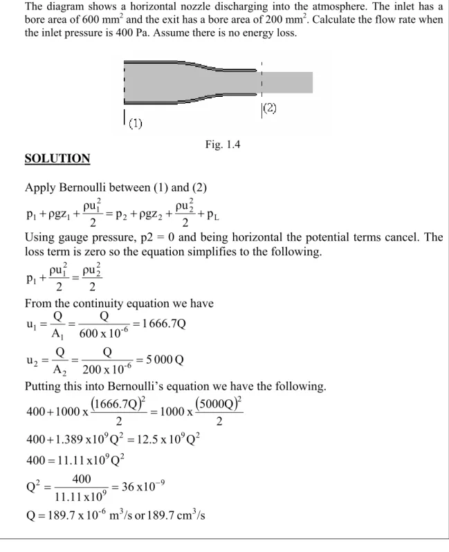
WORKED EXAMPLE 3
The diagram shows a horizontal nozzle discharging into the atmosphere. The inlet has a bore area of 600 mm2 and the exit has a bore area of 200 mm2. Calculate the flow rate when the inlet pressure is 400 Pa. Assume there is no energy loss.
Fig. 1.4
SOLUTION
Apply Bernoulli between (1) and (2) L 2 2 2 2 2 1 1 1 p 2 ρu ρgz p 2 ρu ρgz p + + = + + +
Using gauge pressure, p2 = 0 and being horizontal the potential terms cancel. The loss term is zero so the equation simplifies to the following.
2 ρu 2 ρu p 2 2 2 1 1+ =
From the continuity equation we have
Q 000 5 10 x 200 Q A Q u 666.7Q 1 10 x 600 Q A Q u 6 -2 2 6 -1 1 = = = = = =
Putting this into Bernoulli’s equation we have the following.
(
)
(
)
/s cm 189.7 or /s m 10 x 7 . 189 Q x10 36 x10 11.11 400 Q Q x10 .11 1 1 400 Q 10 x 5 2. 1 Q x10 389 . 1 400 2 5000Q x 1000 2 1666.7Q x 1000 400 3 3 6 -9 9 2 2 9 2 9 2 9 2 2 = = = = = + = + −1.4 HYDRAULIC GRADIENT
Consider a tank draining into another tank at a lower level as shown. There are small vertical tubes at points along the length to indicate the pressure head (h). Relative to a datum, the total energy head is hT = h + z + u2/2g and this is shown as line A.
The hydraulic grade line is the line joining the free surfaces in the tubes and represents the sum of h and z only. This is shown as line B and it is always below the line of hT by the velocity head u2/2g. Note that at exit from the pipe, the velocity head is not recovered but lost as friction as the emerging jet collides with the static liquid. The free surface of the tank does not rise. The only reason why the hydraulic grade line is not horizontal is because there is a frictional loss hf. The actual gradient of the line at any point is the rate of change with length i = δhf/δL
SELF ASSESSMENT EXERCISE 1
1. A pipe 100 mm bore diameter carries oil of density 900 kg/m3 at a rate of 4 kg/s. The pipe reduces to 60 mm bore diameter and rises 120 m in altitude. The pressure at this point is atmospheric (zero gauge). Assuming no frictional losses, determine:
i. The volume/s (4.44 dm3/s)
ii. The velocity at each section (0.566 m/s and 1.57 m/s) iii. The pressure at the lower end. (1.06 MPa)
2. A pipe 120 mm bore diameter carries water with a head of 3 m. The pipe descends 12 m in altitude and reduces to 80 mm bore diameter. The pressure head at this point is 13 m. The density is 1000 kg/m3. Assuming no losses, determine
i. The velocity in the small pipe (7 m/s) ii. The volume flow rate. (35 dm3/s)
3. A horizontal nozzle reduces from 100 mm bore diameter at inlet to 50 mm at exit. It carries liquid of density 1000 kg/m3 at a rate of 0.05 m3/s. The pressure at the wide end is 500 kPa (gauge). Calculate the pressure at the narrow end neglecting friction. (196 kPa)
4. A pipe carries oil of density 800 kg/m3. At a given point (1) the pipe has a bore area of 0.005 m2 and the oil flows with a mean velocity of 4 m/s with a gauge pressure of 800 kPa. Point (2) is further along the pipe and there the bore area is 0.002 m2 and the level is 50 m above point (1). Calculate the pressure at this point (2). Neglect friction. (374 kPa)
5. A horizontal nozzle has an inlet velocity u1 and an outlet velocity u2 and discharges into the atmosphere. Show that the velocity at exit is given by the following formulae.
u2 ={2∆p/ρ + u12}½ and u2 ={2g∆h + u12}½
2 PRESSURE LOSSES IN PIPE SYSTEMS
2 .1 REVIEW OF EARLIER WORK
FRICTION COEFFICIENT
The friction coefficient is a convenient idea that can be used to calculate the pressure drop in a pipe. It is defined as follows.
Pressure Dynamic Stress Shear Wall Cf = p = ½ ρ um2 L p D o 4 ∆ = τ 2 m f u L 4 p D 2 Pressure Dynamic Stress Shear Wall C ρ ∆ = =
From Poiseuille’s equation 2 m D Lu 32 p= µ ∆ Hence e 2 m 2 2 m f R 16 D u 16 D Lu 32 u L 4 D 2 C = ρ µ = ⎟ ⎠ ⎞ ⎜ ⎝ ⎛ µ ⎟⎟ ⎠ ⎞ ⎜⎜ ⎝ ⎛ ρ = DARCY FORMULA D 2 u L C 4 p 2 m f ρ = ∆
This is often expressed as a friction head hf gD 2 Lu C 4 g p h 2 m f f ρ = ∆ =
This is the Darcy formula. In the case of laminar flow, Darcy's and Poiseuille's equations must give the same result so equating them gives
e m f 2 m 2 m f R 16 D u 16 C gD Lu 32 gD 2 Lu C 4 = ρ µ = ρ µ =
This is the same result as before for laminar flow.
A formula that gives an approximate answer for any surface roughness is that given by Haaland.
⎪⎭ ⎪ ⎬ ⎫ ⎪⎩ ⎪ ⎨ ⎧ ⎟ ⎠ ⎞ ⎜ ⎝ ⎛ ε + − = 11 . 1 e 10 f R 3.71 9 . 6 log 6 . 3 C 1
WORKED EXAMPLE 4
Determine the friction coefficient for a pipe 100 mm bore with a mean surface roughness of 0.06 mm when a fluid flows through it with a Reynolds number of 20 000.
SOLUTION
The mean surface roughness ε = k/d = 0.06/100 = 0.0006 Locate the line for ε = k/d = 0.0006.
Trace the line until it meets the vertical line at Re = 20 000. Read of the value of Cf horizontally on the left. Answer Cf = 0.0067
Check using the formula from Haaland.
0067 . 0 C 206 . 12 C 1 71 . 3 0006 . 0 20000 9 . 6 log 6 . 3 C 1 71 . 3 0006 . 0 20000 9 . 6 log 6 . 3 C 1 71 . 3 R 9 . 6 log 6 . 3 C 1 f f 11 . 1 10 f 11 . 1 10 f 11 . 1 e 10 f = = ⎪⎭ ⎪ ⎬ ⎫ ⎪⎩ ⎪ ⎨ ⎧ ⎟ ⎠ ⎞ ⎜ ⎝ ⎛ + − = ⎪⎭ ⎪ ⎬ ⎫ ⎪⎩ ⎪ ⎨ ⎧ ⎟ ⎠ ⎞ ⎜ ⎝ ⎛ + − = ⎪⎭ ⎪ ⎬ ⎫ ⎪⎩ ⎪ ⎨ ⎧ ⎟ ⎠ ⎞ ⎜ ⎝ ⎛ ε + − =
WORKED EXAMPLE 5
Oil flows in a pipe 80 mm bore with a mean velocity of 4 m/s. The mean surface roughness is 0.02 mm and the length is 60 m. The dynamic viscosity is 0.005 N s/m2 and the density is 900 kg/m3. Determine the pressure loss.
SOLUTION
Re = ρud/µ = (900 x 4 x 0.08)/0.005 = 57600
ε= k/d = 0.02/80 = 0.00025 From the chart Cf = 0.0052
hf = 4CfLu2/2dg = (4 x 0.0052 x 60 x 42)/(2 x 9.81 x 0.08) = 12.72 m
2.2 MINOR LOSSES
Minor losses occur in the following circumstances. i. Exit from a pipe into a tank. ii. Entry to a pipe from a tank. iii. Sudden enlargement in a pipe. iv. Sudden contraction in a pipe. v. Bends in a pipe.
vi. Any other source of restriction such as pipe fittings and valves.
Fig.2.1
In general, minor losses are neglected when the pipe friction is large in comparison but for short pipe systems with bends, fittings and changes in section, the minor losses are the dominant factor.
In general, the minor losses are expressed as a fraction of the kinetic head or dynamic pressure in the smaller pipe.
Minor head loss = k u2/2g Minor pressure loss = ½ kρu2
Values of k can be derived for standard cases but for items like elbows and valves in a pipeline, it is determined by experimental methods.
Minor losses can also be expressed in terms of fluid resistance R as follows. 2 4 2 2 2 2 2 L RQ D Q 8 k A 2 Q k 2 u k h = π = = = Hence 2 4 D k 8 R π = 2 4 2 2 L RQ D gQ 8 k p = π ρ = hence 2 4 D g k 8 R π ρ =
Before you go on to look at the derivations, you must first learn about the coefficients of contraction and velocity.
COEFFICIENT OF CONTRACTION Cc
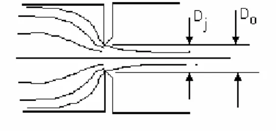
The fluid approaches the entrance from all directions and the radial velocity causes the jet to contract just inside the pipe. The jet then spreads out to fill the pipe. The point where the jet is smallest is called the VENA CONTRACTA.
Fig.2.2
The coefficient of contraction Cc is defined as Cc = Aj/Ao
Aj is the cross sectional area of the jet and Ao is the c.s.a. of the pipe. For a round pipe this becomes Cc = dj2/do2.
COEFFICIENT OF VELOCITY Cv
The coefficient of velocity is defined as Cv = actual velocity/theoretical velocity
In this instance it refers to the velocity at the vena-contracta but as you will see later on, it applies to other situations also.
EXIT FROM A PIPE INTO A TANK.
The liquid emerges from the pipe and collides with stationary liquid causing it to swirl about before finally coming to rest. All the kinetic energy is dissipated by friction. It follows that all the kinetic head is lost so k = 1.0
ENTRY TO A PIPE FROM A TANK
The value of k varies from 0.78 to 0.04 depending on the shape of the inlet. A good rounded inlet has a low value but the case shown is the worst.
Fig.2.4
SUDDEN ENLARGEMENT
This is similar to a pipe discharging into a tank but this time it does not collide with static fluid but with slower moving fluid in the large pipe. The resulting loss coefficient is given by the following expression. 2 2 2 1 1 ⎪⎭ ⎪ ⎬ ⎫ ⎪⎩ ⎪ ⎨ ⎧ ⎟⎟ ⎠ ⎞ ⎜⎜ ⎝ ⎛ − = d d k Fig.2.5 SUDDEN CONTRACTION
This is similar to the entry to a pipe from a tank. The best case gives k = 0 and the worse case is for a sharp corner which gives k = 0.5.
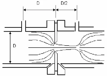
WORKED EXAMPLE 6
A tank of water empties by gravity through a horizontal pipe into another tank. There is a sudden enlargement in the pipe as shown. At a certain time, the difference in levels is 3 m. Each pipe is 2 m long and has a friction coefficient Cf = 0.005. The inlet loss constant is K = 0.3.
Calculate the volume flow rate at this point.
SOLUTION
There are five different sources of pressure loss in the system and these may be expressed in terms of the fluid resistance as follows.
The head loss is made up of five different parts. It is usual to express each as a fraction of the kinetic head as follows.
Resistance pipe A 5 2 6 2 5 2 5 A f 1 1.0328x10 s m 0.02 x g 2 x 0.005 x 32 gD L C 32 R = − π = π = Resistance in pipe B 5 2 5 2 3 2 5 B f 2 4.250x10 s m 0.06 x g 2 x 0.005 x 32 gD L C 32 R = − π = π = Loss at entry K=0.3 4 2 4 2 5 A 2 3 158s m 0.02 x π g 0.3 x 8 D g K 8 R = = − π =
Loss at sudden enlargement. 0.79 60 20 1 d d 1 k 2 2 2 2 B A = ⎪⎭ ⎪ ⎬ ⎫ ⎪⎩ ⎪ ⎨ ⎧ ⎟ ⎠ ⎞ ⎜ ⎝ ⎛ − = ⎪⎭ ⎪ ⎬ ⎫ ⎪⎩ ⎪ ⎨ ⎧ ⎟⎟ ⎠ ⎞ ⎜⎜ ⎝ ⎛ − = 5 2 4 2 4 A 2 4 407.7s m 0.02 x gπ 8x0.79 D gπ 8K R = = = − Loss at exit K=1 2 5 4 2 4 B 2 5 63710s m 0.06 x gπ 8x1 D gπ 8K R = = = − Total losses. 2 6 L 2 5 4 2 2 1 L 2 5 2 4 2 3 2 2 2 1 L Q 10 x 1.101 h )Q R R R R (R h Q R Q R Q R Q R Q R h = + + + + = + + + + = BERNOULLI’S EQUATION
Apply Bernoulli between the free surfaces (1) and (2) L 2 2 2 2 2 1 1 1 h g 2 u z h g 2 u z h + + = + + +
On the free surface the velocities are small and about equal and the pressures are both atmospheric so the equation reduces to the following.
z1 - z2 = hL = 3 3 = 1.101 x 10⁶ Q2 Q2 = 2.724 x 10⁻⁶ Q = 1.65 x 10⁻³ m3/s
2.3 SIPHONS
Liquid will siphon from a tank to a lower level even if the pipe connecting them rises above the level of both tanks as shown in the diagram. Calculation will reveal that the pressure at point (2) is lower than atmospheric pressure (a vacuum) and there is a limit to this pressure when the liquid starts to turn into vapour. For water about 8 metres is the practical limit that it can be sucked (8 m water head of vacuum).
Fig.2.8
WORKED EXAMPLE 7
A tank of water empties by gravity through a siphon. The difference in levels is 3 m and the highest point of the siphon is 2 m above the top surface level and the length of pipe from inlet to the highest point is 2.5 m. The pipe has a bore of 25 mm and length 6 m. The friction coefficient for the pipe is 0.007.The inlet loss coefficient K is 0.7.
Calculate the volume flow rate and the pressure at the highest point in the pipe.
SOLUTION
There are three different sources of pressure loss in the system and these may be expressed in terms of the fluid resistance as follows.
Pipe Resistance 5f 2 5 2 6 2 5 1 1.422 x 10 s m π 0.025 x g 6 x 0.007 x 32 π gD L 32C R = = = −
Entry Loss Resistance 2 2 4 2 4 15.1 x 10³ s2m 5 0.025 x gπ 0.7 x 8 D g K 8 R = = − π =
Exit loss Resistance 3 2 4 2 4 21.57 x 10³ s2m 5 0.025 x g 8x1 D g K 8 R = − π = π = Total Resistance RT = R1 + R2 + R3 = 1.458 x 10⁶ s2 m-5