Article
Py4CAtS—PYthon for Computational
ATmospheric Spectroscopy
Franz Schreier * , Sebastián Gimeno García†, Philipp Hochstaffl and Steffen Städt Deutsches Zentrum für Luft- und Raumfahrt (DLR), Institut für Methodik der Fernerkundung (IMF), 82234 Oberpfaffenhofen, Germany; [email protected] (S.G.G.);
[email protected] (P.H.); [email protected] (S.S.) * Correspondence: [email protected]
† Current address: EUMETSAT, 64283 Darmstadt, Germany.
Received: 5 April 2019; Accepted: 6 May 2019; Published: 10 May 2019 Abstract: Radiation is a key process in the atmosphere. Numerous radiative transfer codes have been developed spanning a large range of wavelengths, complexities, speeds, and accuracies. In the infrared and microwave, line-by-line codes are crucial esp. for modeling and analyzing high-resolution spectroscopic observations. Here we present Py4CAtS—PYthon scripts for Computational ATmospheric Spectroscopy, a Python re-implemen-tation of the Fortran Generic Atmospheric Radiation Line-by-line Code GARLIC, where computationally-intensive code sections use the Numeric/Scientific Python modules for highly optimized array processing. The individual steps of an infrared or microwave radiative transfer computation are implemented in separate scripts (and corresponding functions) to extract lines of relevant molecules in the spectral range of interest, to compute line-by-line cross sections for given pressure(s) and temperature(s), to combine cross sections to absorption coefficients and optical depths, and to integrate along the line-of-sight to transmission and radiance/intensity. Py4CAtS can be used in three ways: in the (Unix/Windows/Mac) console/terminal, inside the (I)Python interpreter, or Jupyter notebook. The basic design of the package, numerical and computational aspects relevant for optimization, and a sketch of the typical workflow are presented. In conclusion, Py4CAtS provides a versatile environment for “interactive” (and batch) line-by-line radiative transfer modeling.
Keywords:infrared; radiative transfer; molecular absorption; line-by-line
1. Introduction
Radiative transfer is an important aspect in various branches of physics, esp. in the atmospheric sciences, both for Earth and (exo-)planets [1–3]. Many radiative transfer models have been developed in recent decades (see [4], for an early review andhttps://en.wikipedia.org/wiki/Atmospheric_ radiative_transfer_codesfor an up-to-date listing (All links in this paper were checked and active 4 April 2019.)), ranging from simple approximations to complex, often highly optimized codes and usually tailored to a specific spectral domain.
An essential prerequisite for the analysis of data recorded by atmospheric remote sensing instruments as well as for theoretical investigations such as retrieval assessments is a flexible, yet efficient and reliable radiative transfer model (RTM). Furthermore, as the retrieval of atmospheric parameters is in general a nonlinear optimization problem (inverse problem), the retrieval code must be closely connected to the radiative transfer code (forward model).
Radiative transfer depends on the state of the atmosphere (pressure, temperature, composition), the optical properties of the atmospheric constituents (molecules and particles), geometry, and spectral range. Because of the numerous parameters the setup of a radiative transfer calculation Atmosphere2019,10, 262; doi:10.3390/atmos10050262 www.mdpi.com/journal/atmosphere
Atmosphere2019,10, 262 2 of 26
can be cumbersome and error prone, and several interfaces have been developed to ease the application. MODO ([5], see alsohttp://www.rese.ch/products/modo/) is a “graphical front-end” to the MODTRAN [6] radiative transfer code, and a Python interface to MODTRAN’s predecessor, the low-resolution band model LOWTRAN, is available athttps://pypi.org/project/lowtran/. Wilson [7], see alsohttp://www.py6s.rtwilson.com/, has developed a Python interface to the widely used 6S (Second Simulation of the Satellite Signal in the Solar Spectrum, [8]) model.
In the infrared and microwave region, line-by-line (lbl) modeling of molecular absorption is mandatory esp. for high spectral resolution. Furthermore, lbl models are required for the setup and verification of fast parameterized models, e.g., band, k-distribution, or exponential sum fitting models [6,9,10]. Moreover, lbl models are ideal for radiative transfer in planetary atmospheres, where fast models often parameterized for Earth-like conditions are not suitable [11,12].
An essential input for lbl radiative transfer codes are the molecules’ optical properties compiled in databases such as HITRAN [13], HITEMP [14], GEISA [15], the JPL and CDMS catalogs [16–18], or ExoMol [19] that list line parameters (center frequency, line strength, broadening parameters etc.) for millions to billions of lines of some dozen molecules. Lbl models are computationally challenging because of the large number of spectral lines to be considered and the large number of wavenumber grid points required for adequate sampling. Nevertheless, lbl models are available for almost half a century, e.g., FASCODE or 4A (Fast Atmospheric Signature Code, Automatized Atmospheric Absorption Atlas, [20,21]). Thanks to the increased computational power (and because of the increased number of high-resolution Earth and planetary spectra) a variety of codes has been developed since these early efforts, e.g., ARTS (Atmospheric Radiative Transfer Simulator, [22–24]), GARLIC (Generic Atmospheric Radiation Line-by-line Code, [25]), GenLN2 [26], KOPRA (Karlsruhe Optimized & Precise Radiative transfer Algorithm, [27]), LblRTM (Line-by-line Radiative Transfer Model, [28]), LinePak [29], RFM (Reference Forward Model, [30]),σ-IASI [31], and VSTAR (Versatile Software for Transfer of Atmospheric Radiation, [32]).
Several web sites offer an Internet access to lbl databases and/or lbl models: “HITRANonline” [33] athttp://hitran.org/allows the downloading of line and other data from the most recent HITRAN version. With the “Information System HITRAN on the Web (HotW)” at http://hitran.tsu.ru
(see also http://spectra.iao.ru/) several types of spectra can be simulated using HITRAN data. The HITRAN Application Programming Interface (HAPI) [34] is “a set of routines in Python which aims to provide remote access to functionality and data given by the HITRANonline”. A similar service (visualization etc.) for the GEISA database is offered athttps://cds-espri.ipsl.upmc.fr/geisa/. The “wavelength search engine” SpectraPlot ([35], see also http://www.spectraplot.com/) is a “web-based application for simulating spectra of atomic and molecular gases” employing, among others, HITRAN and HITEMP.http://www.spectralcalc.com/provides a web interface to the widely used LinePak [29] model (with extended functionality for subscribed users). Goddard’s Planetary Spectrum Generator (PSG,https://psg.gsfc.nasa.gov/, Villanueva et al. [36]) can be used to generate high-resolution spectra of planetary bodies (e.g., planets, moons, comets, exoplanets). Knowledge of the atmospheric transmission is also important for ground-based astronomy observations, and some tools for the correction of telluric absorption are available, e.g., MolecFit ([37], see also
https://www.uibk.ac.at/eso/software/molecfit.html.en) and TAPAS (Transmissions Atmosphériques Personnalisées Pour l’AStronomie, [38], online athttp://cds-espri.ipsl.fr/tapas/) (both codes use LblRTM). An early attempt to a “virtual lab” providing a web interface to MIRART (the Fortran 77 predecessor of GARLIC, [39]) and FASCODE is described in Ernst et al. [40].
In general, RTMs incl. lbl models work as a kind of “black-box”. Given a set of specifications on spectral range, atmospheric conditions, geometry etc. compiled in an input file (or configuration file etc., e.g., theTAPE5used by LOWTRAN, MODTRAN, and FASCODE), the program is executed reading this input file (and probably some further auxiliary files, e.g., the lbl database) and one or several spectra (transmission, radiance, . . . ) are returned (e.g., saved in file(s)). This approach is clearly advantageous when numerous transmission and/or radiance spectra must be generated, e.g., for the
operational analysis of thousands or millions of observed spectra. However, to better understand the physics of radiative transfer, inspection of intermediate variables can provide useful insight. For example, the selection of an appropriate spectral range or measurement geometry is crucial for the design and setup of a new measurement system, and analysis and visualization of line parameters, absorption cross sections and coefficients, layer optical depths, etc. can be useful. Methods and tools have been developed for the “automated” definition of “microwindows”, i.e., spectral intervals optimized for retrieval of temperature or molecular concentrations from thermal emission infrared observations (e.g., [41–46]). Despite these and similar efforts interactive and flexible RTMs with an easy access to all kind of intermediate variables (“step-by-step”, similar to a debugger) appear to be useful, also for pedagogical purposes.
Py4CAtS—Python for Computational Atmospheric Spectroscopy—has been developed with this intention. Since its first release in the mid-1990s [47,48] Python has become increasingly popular for scientific computing [49,50]. Thanks to its numerous extension packages, in particular NumPy/SciPy [51], the “Python-based ecosystem” ([52],https://scipy.org/) is widely considered to be the language of choice in many areas, e.g., atmospheric science and astrophysics [53–55].
Originally, the development of Py4CAtS was motivated by the idea of computational steering [56], i.e., numerically time-consuming tasks such as the lbl evaluation of molecular absorption cross sections are performed by a code (e.g., GARLIC subroutines) written in compiled languages such as Fortran (or C, C++, . . . ) that is made accessible from Python (or another scripting language) using a wrapper such as PyFort [57] or F2Py [58]. More precisely, the intention was to call subroutines of GARLIC from Python. Unfortunately porting the wrapper code from one machine to another turned out to be difficult and time-consuming with early versions of PyFort. However, thanks to the increased performance of NumPy a Python implementation of lbl cross sections became feasible, i.e., the interface to GARLIC’s subroutines became less important. Accordingly, the further development of GARLIC and Py4CAtS became largely independent, and Py4CAtS is now a full lbl radiative transfer tool kit delivering absorption cross sections and coefficients, optical depths, transmissions, weighting functions, and radiances.
The paper is organized as follows: After a brief review of the basic facts of lbl infrared and microwave (for brevity simply IR in the following) radiative transfer in the following section some numerical and implementation aspects are discussed in Section2.2. Usage of the code as well as some implementation details are presented in Section3. The paper continues with a discussion of several aspects in Section4before the final conclusion in Section5. Implementation aspects are described in the AppendixA.
2. Theory and Methods
2.1. Molecular Absorption and Radiative Transfer
Radiative transfer in the IR is essentially described by the Schwarzschild equation and Beer-Lambert law (assuming negligible scattering and local thermal equilibrium in an inhomogeneous atmosphere [1–3]). Given pressurepand temperatureTand line parameters from HITRAN, GEISA, etc. the first step of a simulation is to compute the absorption cross section (xs) for a particular moleculem
km(ν,p,T) =
∑
lSml(T)g(ν; ˆνml,γml(p,T)). (1)
whereνis the wavenumber and the sum comprises all relevant lines characterized by position ˆνml, strengthSml, and broadening parameterγml. The line strengthS(T)at temperatureTis obtained as (note that indices for lines and molecules have been omitted)
S(T) = S(T0)QQ(T0) (T) exp(−Ei/kBT) exp(−Ei/kBT0) 1 − exp(−hcνˆ/kBT) 1 −exp(−hcνˆ/kBT0). (2)
Atmosphere2019,10, 262 4 of 26
with reference strengthS(T0)and lower state energyEifrom the database;Q(T)is the product of rotational and vibrational partition functions (for details see [25], subsection 3.4 or [59]) andc,h, and kBare speed of light, the Planck constant, and the Boltzmann constant, respectively. The combined effect of pressure broadening (corresponding to a Lorentzian profilegL) and Doppler broadening (corresponding to a Gaussian profile gG) is described by a convolution resulting in the Voigt line profile [60]
gV(ν−νˆ,γL,γG) = gL⊗gG = Z ∞
−∞dν
0 gL(ν−ν0,γL) × gG(ν0−νˆ,γG). (3)
The Lorentz and Gauss half widthsγ(at half maximum, HWHM) are pressure- and temperature-dependent, γL = γL0 pp 0 T 0 T n (4) γG = νˆ s 2 ln 2kBT µc2 (5)
where the air-broadening coefficientγ0Land exponentnare given in the database for reference pressure p0and temperatureT0, andµis the molecular mass. Please note that contributions to the Lorentzian width (4) due to self-broadening have been ignored: Except for water at Earth’s bottom of atmosphere (BoA), molecular mixing ratios are usually very small, and the self-broadening contribution would be small to negligible. Moreover, the self-broadening coefficient is often close to the foreign broadening coefficient (or even undefined, at least for older versions of HITRAN and GEISA). Clearly, for planetary atmospheres (e.g., Mars or Venus) self-broadening can be an important issue.
The increasing quality of spectroscopic observations has indicated deficiencies of the Voigt profile, and several more advanced profiles have been suggested [61,62]. In addition to the Lorentz, Gauss, and Voigt profile, implementations of the Rautian and speed-dependent Voigt profile [63] are available. The absorption coefficient (ac) is defined as the sum of all molecular cross sections scaled by the molecular number densitiesnm(in general depending on altitudezand the corresponding pressure)
α(ν,z,p,T) =
∑
m nm(z)km(ν,p(z),T(z)). (6) Integration of the absorption coefficient along the line-of-sight gives the optical depth (od), i.e., for a plane-parallel atmosphere and a vertical path from altitudezlotozhi
τ(ν) =
Z zhi zlo
α(ν,z,p,T)dz. (7)
This is closely related to the monochromatic transmission describing the ratio of incoming and outgoing radiation
T(ν) = exp(−τ(ν)). (8)
Finally, the integral form of Schwarzschild’s equation gives the (spectral) radiance or intensity (ri) I(ν) = Ib(ν)e−τb(ν) + τb Z 0 B(ν,T(τ0))e−τ0dτ0 (9) = Ib(ν)e−τb(ν) − sb Z 0 B(ν,T(s0)) ∂T ∂s0 ds0 (10)
where the first term describes an attenuated background contribution Ib at a distancesb from the observer (corresponding to the optical depthτb), e.g., from Earth’s (or a planet’s) surface in case of nadir-viewing. The source function in the second term is Planck’s function depending on temperature,
B(ν,T) = 2hc
2ν3
exp(hcν/kBT)−1 . (11)
The finite spectral resolution of measured spectra can be modeled by convolution of the monochromatic transmission (8) and/or radiance (9) with an appropriate spectral response function (SRF, a.k.a. instrument line shape, ILS), e.g.,
˜
I= I⊗SRF . (12)
Weighting functions (wf) are an important concept for atmospheric temperature sounding and are a measure of the contribution of a particular atmospheric layer to the radiation seen by an observer, see Equation (10). They are defined by ∂T
∂z for a vertical path, or more generally ∂T(ν,s)
∂s = − T(ν,s)α(ν,s) (13)
for a slant path withs=z/ cosθand zenith angleθ(withθ=0 andθ=180◦for vertical uplooking and downlooking, respectively).
2.2. Numerics
2.2.1. Lbl Molecular Absorption Cross Sections: Multigrid Voigt Function
For the computation of the Voigt profilegV(3) depending on three variables it is convenient to introduce the Voigt functionK(x,y)depending on two variables, essentially the distancexto the center peak and the ratioyof the line widths
gV(ν−νˆ,γL,γG) = √ ln 2/π γG K(x,y) (14) K(x,y) = y π ∞ Z −∞ e−t2 (x−t)2+y2 dt (15)
with x = √ln 2(ν−νˆ)/γG andy = √ln 2γL/γG. As there is no closed-form solution for this convolution integral, numerical approximations are mandatory. Most modern algorithms consider the complex error function [64,65] whose real part is identical to the Voigt function
w(z) ≡ K(x,y) + iL(x,y) = i π Z ∞ −∞ e−t2 z−t dt with z=x+iy. (16) Rational approximations, closely related to continued fractions and defined as the quotient of two polynomials [66,67], have been used successfully for a large variety of functions including the complex error function (e.g., [68–70]). Py4CAtS (like GARLIC) uses an optimized combination [71] of the Humlíˇcek [69] and Weideman [70] algorithms
w(z) = iz/√π z2−1 2 |x|+y>15 π−1/2 L−iz + (L−2iz)2 N−1 ∑ n=0an+1Z n otherwise (17)
Atmosphere2019,10, 262 6 of 26
where Z = LL+−iziz and L = 2−1/4N1/2. For N = 24 this provides an accuracy better than 10−4 everywhere except for very smallyand intermediatexthat are hardly relevant in practice; forN=32 the relative error|∆K|/Kis less than 8×10⁻⁵for allx,yof interest.
Because of the huge number of Voigt function evaluations even highly optimized complex error function algorithms are insufficient and further optimizations are mandatory. Py4CAtS evaluates the monochromatic cross sections on a uniform (equidistant) wavenumber grid with the spacing estimated as a fraction of the “typical” line widths, i.e.,δν=hγi/nwith the mean half widthhγiand a default sampling raten=4. In case of the Voigt line profile (3), its width is estimated using an approximation due to Whiting [72] (accurate to about one percent)
γV ≈ 12
γL+ q
γ2L+4γ2G. (18)
Please note thatδνand hence the number of grid points and cross section values are dependent on pressure, temperature, and molecular mass (via Equations (4), (5), and (18)), and change with atmospheric level and molecule. These wavenumber steps are clearly appropriate in the line center region; however, in the line wings the profiles are relatively smooth (roughlyg(ν−νˆ)≈1/(ν−νˆ)2
for the Lorentz or Voigt profile) and a coarser grid would be sufficient.
Py4CAtS uses a two- or three-grid approach [73]. In the two-grid scheme, the Voigt line profile is calculated on the fine grid only in the line center region, and on a coarse grid (typically with spacing
∆ν=8δν) in the entire spectral region. The line profiles are accumulated independently to the fine and coarse grid cross sections, i.e., the interpolation of the coarse grid cross section is done only once after all lines have been summed up. This allows a speed-up roughly in the order of the ratio of fine and coarse grid points. A significant further speed-up can be achieved with three grids of fine, medium, and coarse resolution and exploitation of the asymptotic properties of the profile function.
2.2.2. Integration of the Beer and Schwarzschild Equations
From the very beginning of the code development (MIRART, GARLIC, and Py4CAtS) numerical schemes have been used whenever possible. Hence, in contrast to most lbl radiative transfer codes dividing the atmosphere into a series of layers with constant pressure, temperature, and concentrations (Curtis-Godson approximation), Py4CAtS and GARLIC are level-based and exploit numerical quadrature for Equations (7) and (9). In particular, the optical depth is approximated by the sum of absorption coefficients according to the trapezoid rule (e.g., [66]). For the Schwarzschild Equation (9) both codes use optical depthτas integration variable and assume that the Planck function varies linearly or exponentially with optical depth within a layer,
B(τ) = b0B(τl) +b1B(τl+1) withb0= τl+1−τ
τl+1−τl andb1=
τ−τl
τl+1−τl (19) B(τ) = B(τl)eβ(τ−τl) withβ=log B(τl)/B(τl+1)/(τl+1−τl) (20) forτl ≤τ≤τl+1(corresponding to the altitude interval[zl,zl+1]). Note the slightly different notation for the Planck function’s argument here compared to Equation (11) (the optical depth depends on wavenumber and temperature). With both approximations the integral (9) can be computed analytically within a layer.
Because the overall runtime is essentially determined by the evaluation of the cross sections, the speed of level-based and layer-based radiative transfer is equivalent (assuming that the number of levels and layers is comparable). With respect to accuracy, none of the two approaches is superior or inferior; in fact, neither of the intercomparison studies [74–76] identified path integration as an issue. For an in-depth discussion of the “linear-in-τ” vs. “exponential-in-τ” approximations as well as some further quadrature schemes see subsection 4.1 of the GARLIC paper [25].
3. The Package: Usage and Implementation
In Py4CAtS the individual steps of an IR radiative transfer computation are implemented in a series of modules and functions, see Figure1:
• higstract: extract (select) lines of relevant molecules in the spectral range of interest; • lbl2xs: compute lbl cross sections for given pressure(s) and temperature(s): Equation (1); • xs2ac: multiply cross sections with number densities and sum over all molecules: Equation (6); • ac2od: integrate absorption coefficients along the line-of-sight through the atmosphere to the
vertical optical depth (7);
• od2ri: solve Schwarzschild equation (9), i.e., integrate the Planck function (11) vs. optical depth along the line-of-sight through atmosphere (assuming a plane-parallel, non-scattering atmosphere in local thermal equilibrium).
Version May 3, 2019 submitted toAtmosphere 7 of 26
lines xs ac od ri
higstract lbl2xs xs2ac ac2od od2ri lbl2od
lbl2ac xs2od
wf
ac2wf
p,T VMR Geo
Figure 1.From Hitran/Geisa via cross sections (xs) and absorption coefficients (ac) to optical depths (od) and radiation intensity (ri). Note that cross sections are pressure and temperature(pT)dependent, absorption coefficients also depend on composition(VMR), and optical depth and radiation intensity depends on path geometry(geo).
• od2ri: solve Schwarzschild equation (9), i.e. integrate the Planck function vs. optical depth along 215
the line-of-sight through atmosphere (assuming a plane-parallel, non-scattering atmosphere in 216
local thermal equilibrium). 217
All Python source files along with supplementary files are delivered as a single tarball. Unpacking 218
this file will create four directories with the source files insrc, data indata, documentation indoc, 219
and executable scripts in bin. Actually the files in thebin directory are just links to the scripts 220
in thesrcdirectory (e.g.bin/lbl2xsis a link tosrc/lbl2xs.py), and in the following subsection 221
it is assumed that the bin directory is included in the shell’s search path for executables (PATH 222
environment variable for Unix like systems). When Py4CAtS is used inside the IPython interpreter 223
(see Subsection3.2), all functions etc. should have been imported using a statement such as%run 224
/home/schreier/py4cats/src/py4cats.py. Importing Py4CAtS can be easily done automatically by 225
an appropriate modification of the (I)Python configuration file, e.g. by adding this file to the list of files 226
to run at IPython startup3
227
3.1. Running Py4CAtS in the Classical Console 228
A typical session in a Unix/Linux environment (console/terminal) is shown in Fig.2. After 229
creating a new directory the first step is to extract the relevant lines from the HITRAN or GEISA data 230
base4usinghigstract. Note that for this command at least one option is mandatory, i.e. the spectral
231
range (here 50 to 60 cm−1) or a molecule has to be specified (for convenience,higstract -m main ...
232
can be used to extract line data for the first seven molecules (H2O, CO2, . . . , O2) of HITRAN or GEISA.)
233
higstractsaves the data in several tabular ASCII files, one file per molecule. By default, each file has 234
five columns for line position ˆν, strengthsS, energyE, air-broadening parameterγ0L, and the exponent
235
nand is named asH2O.vSEanetc., where the extension indicates the columns (further parameters, e.g. 236
for self-broadening, can be requested with the format option-f). 237
The next step is to compute absorption cross sections according to Eq. (1). Without any option, 238
cross sections are computed for the reference pressure and temperature used in the line parameter 239
database, i.e.p0=1013.25 mb andT0=296 K for HITRAN and GEISA. Alternatively, pressure(s) and
240
temperature(s) can be specified with the-pand-Toption. For atmospheric applications it is more 241
convenient to read the data from a file (e.g. “midlatitude summer” (mls) data assuming the first three 242
3 In IPython 6 this list is defined byc.InteractiveShellApp.exec_filesin.ipython/profile_default/iypthon_config.py.
4 Data are available athitran.organdhttp://cds-espri.ipsl.upmc.fr/. Py4CAtS can read the original data file as is, i.e. the
160-byte fixed-width format used since HITRAN 2004 (or the 100-byte format of the older HITRAN versions). Regarding GEISA, the format of a single record (corresponding to a “physical line”) has changed slightly from version to version, and Py4CAtS parses the file name to select the appropriate reader.
Figure 1. From HITRAN/GEISA via cross sections (xs) and absorption coefficients (ac) to optical depths (od) and radiation intensity (ri). Please note that cross sections are pressure and temperature (pT) dependent, absorption coefficients also depend on composition (VMR), and optical depth and radiation intensity depends on path geometry (geo).
All Python source files along with supplementary files are delivered as a single tarball. Unpacking this file will create four directories with the source files insrc, data indata, documentation indoc, and executable scripts inbin. Actually, the files in thebindirectory are just links to the scripts in the srcdirectory (e.g., bin/lbl2xs is a link to src/lbl2xs.py), and in the following subsection it is assumed that the bindirectory is included in the shell’s search path for executables (PATH environment variable for Unix-like systems). When Py4CAtS is used inside the IPython interpreter (see Section 3.2), all functions etc. should have been imported using a statement such as %run /home/schreier/py4cats/src/py4cats.py. Importing Py4CAtS can be easily done automatically by an appropriate modification of the (I)Python configuration file, e.g., by adding this file to the list of files to run at IPython startup. (In IPython 6 this list is defined byc.InteractiveShellApp.exec_filesin .ipython/profile_default/iypthon_config.py.)
3.1. Running Py4CAtS in the Classical Console
A typical session in a Unix/Linux environment (console/terminal) is shown in Figure2. After creating a new directory, the first step is to extract the relevant lines from the HITRAN or GEISA data base usinghigstract. (Data are available athitran.organdhttp://cds-espri.ipsl.upmc.fr/. Py4CAtS can read the original data file as is, i.e., the 160-byte fixed-width format used since HITRAN 2004 or the 100-byte format of the older HITRAN versions. Regarding GEISA, the format of a single record (corresponding to a “physical line”) has changed slightly from version to version, and Py4CAtS parses the file name to select the appropriate reader.) Please note that for this command at least one option is mandatory, i.e., the spectral range (here 50 to 60 cm−1) or a molecule must be specified (for convenience,higstract -m main ...can be used to extract line data for the first seven molecules (H2O, CO2, . . . , O2) of HITRAN or GEISA.)higstractsaves the data in several tabular ASCII files, one file per molecule. By default, each file has five columns for line position ˆν, strengthsS, energyE,
Atmosphere2019,10, 262 8 of 26
air-broadening parameterγ0L, and the exponentnand is named asH2O.vSEanetc., where the extension indicates the columns (further parameters, e.g., for self-broadening, can be requested with the format
optionVersion May 3, 2019 submitted to-f). Atmosphere 8 of 26
mkdir example; cd example
higstract -x 50,60 /data/hitran/2000/lines
lbl2xs H2O.vSEan CO2.vSEan O3.vSEan # one cross section per molecule at HITRAN p, T lbl2xs -o xSec --pT /data/atmos/mls.xy --cpT 1,2 H2O.vSEan CO2.vSEan O3.vSEan xs2od -o mls.od /data/atmos/mls.xy H2O.xSec CO2.xSec O3.xSec
od2ri -o mls_uplook.ri mls.od # default zenith angle 0dg, downwelling radiation
od2ri -o mls_nadir.ri -T 294 -z 180 mls.od # observer @ ToA, upwelling rad. incl. surface # bypassing the cross section and absorption coefficient file I/O
lbl2od -o mls.od /data/atmos/mls.xy H2O.vSEan CO2.vSEan O3.vSEan
Figure 2.Typical workflow for lbl modelling with Py4CAtS in a Unix-like shell: Hitran/Geisa→line parameter extracts→cross sections→absorption coefficients→optical depth→radiance / intensity. Output is not shown. All functions support the-hoption to ask for help, in particular a list of all available options/flags. For some notes on option parsing see AppendixA.7.
column list altitudes, pressure, and temperature). Again, the cross sections will be saved in files, one 243
per molecule, using NumPy’s pickle format or alternatively ASCII tabular or HITRAN formatted files. 244
The computation continues to absorption coefficients by summing all cross sections (level-by-level) 245
scaled with the molecular concentrations, cf. Eq. (6), and integrating these to the layer (or delta) optical 246
depth, Eq. (7). Finally, the radiance seen by an observer at ground and by a spaceborne observer 247
(actually an observer at top-of-atmosphere, ToA) is computed. 248
In each step of the calculation the results are written to file(s), and read in for the next step. 249
Obviously this can be quite time-consuming esp. for ASCII files (reading NumPy pickled files is 250
surprisingly fast). In particular, the cross section files can be very large (depending on the spectral 251
region, the size of the spectral interval, the number of molecules and atmospheric levels, etc.). For many 252
applications some of the intermediate quantities are not of interest, and the file transfer operations can 253
be omitted, e.g.(see the dashed arrows in Fig.2)
254
• lbl2ac compute lbl cross sections and combine to absorption coefficients; 255
• lbl2od compute lbl cross sections and absorption coefficients, then integrate to optical depth. 256
• xs2od multiply cross sections with densities, sum over molecules, and integrate to optical 257
depth. 258
In addition to these scripts there are several further Python files that contain functions used by 259
these “main” scripts (e.g. to read or write the data), but can also be executed stand-alone.5lines.py,
260
xSection.py,absCo.py,oDepth.pycan be used to read, extract subsets in the spectral or altitude 261
regime, summarize, plot, or reformat the respective data. molecules.pycollects properties (e.g. 262
mass) of the IR relevant molecules and also the ID numbers used in the HITRAN and GEISA database. 263
atmos1D.pyis useful to handle the atmospheric data (p,T, VMRs, . . . ). The functions inhitran.pyand 264
geisa.pyare used byhigstract.py, but can be used as a “low-level” interface to the respective dataset. 265
Unit conversions are implemented in thecgsUnit.pymodule (note that internally Py4CAtS uses cgs 266
units consistently,see AppendixA.6). Furthermore,radiance2radiance.pyandradiance2Kelvin.py 267
allow the conversion of radiance spectra, e.g. wavenumber←→wavelength or to equivalent brightness 268
temperature using the inverse of Planck’s function (11). 269
Thelbl2ac,lbl2od, orxs2odscripts clearly help to avoid the time-consuming reading and 270
writing of some of the intermediate quantities, however, these scripts turn Py4CAtS back into the 271
“black-box” radiative transfer discussed above. 272
5 Technically, the very first line of all executable scripts is something like#!/usr/bin/env pythonand the last segment of
the module starts withif __name__==’__main__’:.
Figure 2.Typical workflow for lbl modeling with Py4CAtS in a Unix-like shell: Hitran/Geisa→line parameter extracts→cross sections→absorption coefficients→optical depth→radiance / intensity. Output is not shown. All functions support the-hoption to ask for help, in particular a list of all available options/flags. For some notes on option parsing see AppendixA.7.
The next step is to compute absorption cross sections according to Equation (1). Without any option, cross sections are computed for the reference pressure and temperature used in the line parameter database, i.e., p0 = 1013.25 mb andT0 = 296 K for HITRAN and GEISA. Alternatively, pressure(s) and temperature(s) can be specified with the-pand-Toption. For atmospheric applications it is more convenient to read the data from a file (e.g., “midlatitude summer” (mls) data assuming the first three column list altitudes, pressure, and temperature). Again, the cross sections will be saved in files, one per molecule, using NumPy’s pickle format or alternatively ASCII tabular or HITRAN formatted files.
The computation continues to absorption coefficients by summing all cross sections (level-by-level) scaled with the molecular concentrations, cf. Equation (6), and integrating these to the layer (or delta) optical depth, Equation (7). Finally, the radiance seen by an observer at ground and by a spaceborne observer (actually an observer at top of atmosphere, ToA) is computed.
In each step of the calculation the results are written to file(s), and read in for the next step. Obviously, this can be quite time-consuming esp. for ASCII files (reading NumPy pickled files is surprisingly fast). In particular, the cross section files can be very large (depending on the spectral region, the size of the spectral interval, the number of molecules, and atmospheric levels, etc.). For many applications some of the intermediate quantities are not of interest, and the file transfer operations can be omitted, e.g., (see the dashed arrows in Figure2)
• lbl2ac compute lbl cross sections and combine to absorption coefficients;
• lbl2od compute lbl cross sections and absorption coefficients, then integrate to optical depth. • xs2od multiply cross sections with densities, sum over molecules, and integrate to optical depth.
In addition to these scripts there are several further Python files that contain functions used by these “main” scripts (e.g., to read or write the data), but can also be executed stand-alone. (Technically, the very first line of all executable scripts is something like#!/usr/bin/env pythonand the last segment of the module starts withif __name__==’__main__’:.) The scriptslines.py,xSection.py, absCo.py,oDepth.pycan be used to read, extract subsets in the spectral or altitude regime, summarize, plot, or reformat the respective data.molecules.pycollects properties (e.g., mass) of the IR relevant molecules and the ID numbers used in the HITRAN and GEISA database.atmos1D.pyis useful to handle the atmospheric data (p,T, VMRs, . . . ). The functions inhitran.pyandgeisa.pyare used by higstract.py, but can be used as a “low-level” interface to the respective dataset. Unit conversions are implemented in thecgsUnit.pymodule (note that internally Py4CAtS uses cgs units consistently, see AppendixA.6). Furthermore,radiance2radiance.pyandradiance2Kelvin.pyallow the conversion
of radiance spectra, e.g., wavenumber←→wavelength or to equivalent brightness temperature using the inverse of Planck’s function (11).
Thelbl2ac,lbl2od, or xs2odscripts clearly help to avoid the time-consuming reading and writing of some of the intermediate quantities, however, these scripts turn Py4CAtS back into the “black-box” radiative transfer discussed above.
When executing the series of individual steps, the subsequent steps must re-read the data saved in the previous step(s) from file(s) and check the consistency of the data. For example, thexs2ac.pyscript will test if all cross sections cover the same spectral interval, and if the pressures and temperatures match those in the atmospheric data file. Accordingly, a substantial part of the code is devoted to implement appropriate tests. A prerequisite for these tests is that all relevant attributes are saved in the file along with the spectra; for example, a single cross section is saved along with its pressure, temperature, and wavenumber grid specification.
3.2. Py4CAtS Used within the (I)Python and Jupyter Shell
Access to intermediate quantities is especially useful for visualization. In the (I)Python interpreter, graphics packages such as Matplotlib [77] allow the plotting of any kind of array. For plotting as well as for the subsequent processing steps it is important to have all attributes of a spectrum available. However, a function returning an array for the spectrum together with its attributes (e.g., with a call such aslines_h2o, pRef, tRef = higstract(’/data/hitran/86/lines’, ’H2O’)) would be cumbersome, and collecting the return values in a dictionary would not significantly improve this. In Py4CAtS this problem is solved by means of subclassed and/or structured NumPy arrays that will be briefly described (in AppendicesA.4andA.5) after a presentation of the typical workflow illustrated in Figure3.
3.2.1. Atmospheric Data
Knowledge of the atmospheric state, i.e., pressure, temperature, and molecular composition as a function of altitude, is indispensable for lbl modeling and radiative transfer. The Py4CAtS scripts called from the console automatically read these data from a file (along with the line data, cross section data, etc.) This is essentially accomplished by the functionatmReadof theatmos1D.pymodule, e.g., the commandmls = atmRead(’/data/atmos/20/mls.xy’)returns the data of the “midlatitude summer” atmosphere of the AFGL dataset [78] regridded to 20 levels (see the very first input labelled In[1]: in Figure 3). atmReadessentially expects a tabular ascii file with rows corresponding to the atmospheric levels and columns for altitudes, pressure (and/or air density), temperature, and molecular concentrations. Two comment lines are mandatory: #what: followed by the column identifiers and#units:followed by the physical units (e.g., “km”).
mlsis an example of a structured array (see AppendixA.5), where the individual profiles can be accessed by their name, e.g.,mls[’T’]ormls[’H2O’], and the data for a specific levellare given by the row index, e.g.,mls[0]ormls[-1]for the bottom and top level, respectively. Please note that “rows” and “columns” can be specified in two ways; for example, the BoA temperature ismls[’T’][0]
AtmosphereVersion May 3, 2019 submitted to2019,10, 262 Atmosphere 9 of 2610 of 26
Jupyter QtConsole 4.3.1
Python 3.6.5 (default, Mar 31 2018, 19:45:04) [GCC] In[1]: # get two mid latitude atmospheres
...: mls = atmRead('/data/atmos/20/mls.xy')
...: mlw = atmRead('/data/atmos/25/mlw.xy', zToA=50) Atmos1d: got p, T, air and 7 gases at 20 levels Atmos1d: got p, T, air and 7 gases at 18 levels In [2]: # HItran-GeiSa-exTRACT ---> lineListDictionary
...: llDict = higstract('/data/geisa/87/lines', (2100,2150), molecule='main')
9771 lines of 5 molecule(s), returning a dictionary
In [3]: # CO cross section at database pressure and temperature ...: xs = lbl2xs(llDict['CO'])
...: # cross sections for other pressures or temperatures ...: xs_10mb = lbl2xs(llDict['CO'], 1e4) # p=10mb
...: xss = lbl2xs(llDict['CO'], temperature=[200,250,300])
...: # a dictionary of x-section lists (for all p, T and gases) ...: xssDict = lbl2xs(llDict, mls['p'], mls['T'])
In [4]: # proceed step-by-step
...: acList = xs2ac(mls, xssDict) # absorption coefficients ...: dodList = ac2dod(acList) # delta optical depths In [5]: # alternatively bypass intermediate quantities, e.g.
...: dodList = lbl2od(mls,llDict) # delta opt.depths In [6]: # sum/combine optical depths and plot
...: odPlot([dodList[0], dodList[1]]) # the bottom layers ...: odPlot(dodList[0]+dodList[1]) # and their sum In [7]: # radiation intensity seen by uplooking observer at BoA
...: radUp = dod2ri(dodList)
...: # and downlooking observer at ToA (incl. surface @ 294K) ...: radNadir = dod2ri(dodList, 180, mls['T'][0])
Figure 3.Typical workflow of an IPython session (output not shown except for first two commands). When executing the series of individual steps, the subsequent steps have to re-read the data 273
saved in the previous step(s) from file(s) and check the consistency of the data. For example, the 274
xs2ac.pyscript will test if all cross sections cover the same spectral interval, and if the pressures and 275
temperatures match those in the atmospheric data file. Accordingly, a substantial part of the code is 276
devoted to implement appropriate tests. A prerequisite for these tests is that all relevant attributes 277
are saved in the file along with the spectra; for example, a single cross section is saved along with its 278
pressure, temperature, and wavenumber grid specification. 279
3.2. Py4CAtS used within the (I)Python and Jupyter Shell 280
Access to intermediate quantities is especially useful for visualization. In the (I)Python interpreter, 281
graphics packages such as Matplotlib [77] allow to plot any kind of array. For plotting as well as 282
for the subsequent processing steps it is important to have all attributes of a spectrum available. 283
However, a function returning an array for the spectrum together with its attributes (e.g. with a 284
call such aslines_h2o, pRef, tRef = higstract(’/data/hitran/86/lines’, ’H2O’)) would be 285
cumbersome, and collecting the return values in a dictionary would not significantly improve this. In 286
Py4CAtS this problem is solved by means of subclassed and/or structured NumPy arrays that will be 287
Figure 3.Typical workflow of an IPython session (output not shown except for first two commands). All data are stored internally in cgs units, e.g., pressure is converted to dyn/cm2 =g/cm/s2. Molecular concentrations are stored as number densities (i.e., if the data file contains volume mixing ratios (VMR), these are converted to densities by multiplication with the air number density n=p/(kT)). VMR can be obtained with the vmrfunction, e.g., vmr(mls). Further convenience functions of theatmos1D.pymodule includevcdto integrate the (molecular and air) number densities along a vertical path through the atmosphere to the “Vertical Column Density” (N=R
n(z)dzwith default limits given by top and bottom of atmosphere,zToAandzBoA),cmrfor the “Column Mixing Ratio”, i.e., the ratio of the molecular VCDs and the air VCD.
TheatmRegrid (mls, zNew, ...) function allows interpolation of the atmospheric data to a new altitude grid. If the limits of the new grid exceed the old limits,atmRegridprints a warning. The actual results are depending on the chosen interpolation scheme; in case of the default linear interpolation NumPy’sinterpfunction simply repeats the very first or last value at BoA or ToA, respectively.
Data from different files can be combined with theatmMergefunction, e.g.,
combiAtm = atmMerge (mlw, traceGases) (here the second data set “traceGases” is likely comprising only concentration profiles that can be read with thevmrReadfunction.) If the two data sets are given on different altitude grids, profiles from the second set are interpolated to the grid of
the first set. If a profile is defined in both data, then by default the second is ignored unless the flag replaceis “switched on”.
The data can be easily visualized using the standard Matplotlib [77] functions (e.g., plot(mls[’T’],mls[’z’])), but for convenience Py4CAtS provides a function atmPlot that expects a single structured array or a list thereof as first argument. (For some general remarks on visualization see AppendixA.2.) For example,atmPlot(mls)shows temperature vs. altitude, and atmPlot([mls,mlw], ’O3’, ’mb’)compares ozone profiles of the midlatitude summer and winter atmospheres with pressure as vertical axis. Finally, the functionatmSavecan be used to write the data to file (see also AppendixA.1).
3.2.2. Line Data
For the following presentation assume that you are interested in carbon monoxide (CO) retrievals from the thermal IR observations as done by IASI (e.g., [79,80]) or AIRS [81].
llDict = higstract(’/data/hitran/2012/lines’, (2100,2150))returns about 26 thousand lines in a dictionary of 22 line lists, more precisely structured arrays, one array for each molecule with transitions in this spectral range around the CO fundamental band around 2143 cm−1. Actually, these arrays are subclassed NumPy arrays (with typelineArray) holding some extra information as attributes, e.g.,llDict[’CO’].pandllDict[’CO’].tgives HITRAN’s reference pressure 1013.25× 103dyn/cm2 and temperature 296.0 K, respectively. If lines of a single molecule are extracted (e.g., higstract(’/data/geisa/2003/lines’, molecule=’CO’)), a single lineArray is returned. The option molecule=’main’returns the line parameters of the “main” molecules only, i.e., the molecules with ID numbers≤7 of the HITRAN and GEISA database.
Similar to the atmospheric data, the line data can be plotted using Matplotlib’s functions, or, more conveniently, with Py4CAtS’ function, e.g.,atlas(llDict). Theatlasfunction (named after Park et al. [82]) can be used with a singlelineArrayor a list or dictionary oflineArrays and displays line strength vs. position by default.
3.2.3. Cross Sections
In the next step the line parameters can be used to compute molecular cross sections, see the In[3]:block in Figure3.xs = lbl2xs(llDict[’CO’])returns the cross section of CO in the spectral range around 2140 cm−1for the database (here HITRAN) reference pressure and temperature. A single cross section is stored in a subclassed NumPy array (i.e.,type(xs) → xsArray) with “attributes” such as lower and upper wavenumber bound, pressure, temperature, and molecule stored in further items, e.g.,xs.xorxs.p. As a default, the Voigt profile is considered. Please note that the cross sections are evaluated on a uniform wavenumber grid (with spacing defined by the mean line width, see Section2.2.1), so it is sufficient (and more memory efficient) to save the very first and very last grid point only.
Cross sections for different pressures and temperatures are obtained by specifying the second or third function argument oflbl2xs. Please note that the data type returned bylbl2xsin these examples is different, i.e., the type is depending on the number ofp,Tpairs and the type of the line data (a single or a dictionary oflineArray, essentially the number of molecules). In the very first example (CO and onep,T) in Figure3a single subclassed NumPy arrayxsArrayis returned, whereas a list ofxsArray’s is returned for a list ofp,Tpairs and a single molecule. Finally, the last example gives a dictionary of lists ofxsArray’s, each list for a single molecule and a dictionary entry for each molecule.
ThexSection.pymodule has a functionxsPlotto visualize the cross sections, e.g.,xsPlot(xss). This function works recursively (cf. AppendixA.3), i.e., it can be called with a singlexsArray, a list thereof, or a dictionary of (lists of)xsArray’s. Figure4demonstrates the combined use of theatlas andxsPlotfunctions exploiting Matplotlib’s functiontwinxto share the common wavenumber axis. The functionsxsInfoandxsSavecan be used with a single cross section array, a list of cross sections,
Atmosphere2019,10, 262 12 of 26
or a dictionary of lists to summarize the cross sections’ properties or to write the data to file(s); Reading cross section data from file(s) is possible with thexsReadfunction.
Version May 3, 2019 submitted toAtmosphere 11 of 26
4275 4280 4285 4290 4295 4300 4305 4310 position ˆν[cm−1] 10−35 10−33 10−31 10−29 10−27 10−25 10−23 10−21 Strength S [cm − 1/ (molec . cm − 2)] CO p=1e+06 T=296.0 85 H2O p=1e+06 T=296.0 162 CH4 p=1e+06 T=296.0 246 N2O p=1e+06 T=296.0 3 10−28 10−27 10−26 10−25 10−24 10−23 10−22 10−21 10−20 cross section k ( ν ) [cm 2/ molec] 1.01e+03mb 296.00K CO 1.01e+03mb 296.00K H2O 1.01e+03mb 296.00K CH4 1.01e+03mb 296.00K N2O
Figure 4.Combination of line atlas and xsPlot. This example has been generated with
dll = higstract(’/data/hitran/2000/lines’,(4273,4312), ’main’) # dict of line lists xss = lbl2xs(dll) # dict of cross sections
atlas(dll); twinx(); xsPlot(xss)
with transitions in this spectral range around the CO fundamental band around 2143 cm−1. Actually,
336
these arrays are subclassed NumPy arrays (with typelineArray) holding some extra information as 337
attributes, e.g. llDict[’CO’].pandllDict[’CO’].tgives HITRAN’s reference pressure 1013.25 · 338
103dyn/cm2and temperature 296.0 K, respectively. If lines of a single molecule are extracted (e.g.,
339
higstract(’/data/geisa/2003/lines’, molecule=’CO’)), a singlelineArrayis returned. The 340
optionmolecule=’main’returns the line parameters of the “main” molecules only, i.e. the molecules 341
with ID numbers≤7 of the HITRAN and GEISA database. 342
Similar to the atmospheric data, the line data can be plotted using Matplotlib’s functions, or, more 343
conveniently, with Py4CAtS’ function, e.g. atlas(llDict). Theatlasfunction (named after Park 344
et al.[82]) can be used with a singlelineArrayor a list or dictionary oflineArrays and displays line 345
strength vs. position by default. 346
3.2.3. Cross Sections 347
In the next step the line parameters can be used to compute molecular cross sections, see the 348
In[3]:block in Fig.3. xs = lbl2xs(llDict[’CO’]) returns the cross section of CO in the spectral 349
range around 2140 cm−1for the database (here HITRAN) reference pressure and temperature. A single
350
cross section is stored in a subclassed NumPy array (i.e.type(xs) → xsArray) with “attributes” such 351
as lower and upper wavenumber bound, pressure, temperature, and molecule stored in further items, 352
e.g.xs.xorxs.p.As a default, the Voigt profile is considered.Note that the cross sections are evaluated 353
on a uniform wavenumber grid (with spacingdefined by the mean line width, see subsection2.2.1), so 354
it is sufficient (and more memory efficient) to save the very first and very last grid point only. 355
Cross sections for different pressures and temperatures are obtained by specifying the second or 356
third function argument oflbl2xs. Note that the data type returned bylbl2xsin these examples is 357
different, i.e. the type is depending on the number ofp,Tpairs and the type of the line data (a single 358
or a dictionary oflineArray, essentially the number of molecules). In the very first example (CO and 359
onep,T) in Fig.3a single subclassed NumPy arrayxsArrayis returned, whereas a list ofxsArray’s is 360
returned for a list ofp,Tpairs and a single molecule. Finally, the last example gives a dictionary of 361
lists ofxsArray’s, each list for a single molecule and a dictionary entry for each molecule. 362
ThexSection.pymodule has a functionxsPlotto visualize the cross sections, e.g. xsPlot(xss). 363
This function works recursively(cf. AppendixA.3), i.e. it can be called with a singlexsArray, a list 364
Figure 4.Combination of line atlas and xsPlot. This example has been generated with
dll = higstract(’/data/hitran/2000/lines’,(4273,4312), ’main’) # dict of line lists xss = lbl2xs(dll) # dict of cross sections
atlas(dll); twinx(); xsPlot(xss)
.
3.2.4. Absorption Coefficients
Given cross sections of some molecules on a set ofp,Tlevels along with the atmospheric data, in particular the molecular number densities, the absorption coefficient (6) for all levels are generated withacList = xs2ac (mls, xssDict). The list contains a spectrum for each atmosphericp,Tlevel, where each spectrum is stored in a subclassed NumPy array:type(acList[0]) → acArraysimilar to the cross sections, i.e., with attributes stored as, e.g.,ac.xandac.zfor the wavenumber range and altitude, respectively. Please note that the number of levels in the atmospheric data set (heremls) and the lengths of the cross section lists in thexssDictdictionary must be identical. Furthermore, all molecules with cross section data must be contained in the atmospheric data (but there can be some “unused” molecules in the atmospheric data set).
The absorption coefficients can be plotted with the standard Matplotlib functions, but Py4CAtS also has a function to make this easier:acPlot(acList). The functionacInfo(acList)prints essential information about the absorption coefficients (Actually it is a loop calling the correspondinginfo method ofacArray, i.e.,for ac in acList: ac.info()).
The data can be saved to file (tabular ascii) with the standard NumPysavetxtor Py4CAtS’ awritefunction. TheacSavefunction automatically saves the absorption coefficients along with the atmospheric data, and the acRead function allows reading of the data (incl. the associated atmosphere) back from file, e.g.,absCo = acRead(acFile). BothacSaveandacReadalso support HITRAN formatted files or Python/NumPy’s internal pickle format.
3.2.5. Optical Depths
The next step is to integrate the absorption coefficients along the (vertical) path through the atmosphere using the functionac2dod(seeIn[4]in Figure3). Similar to cross sections and absorption coefficients this returns a list of(nLevels-1)subclassed NumPy arrays odArray, where each list member is essentially the delta / differential / layer optical depth spectrum along with its attributes lower and upper altitudes, pressures, and temperatures (and the wavenumber interval, too).
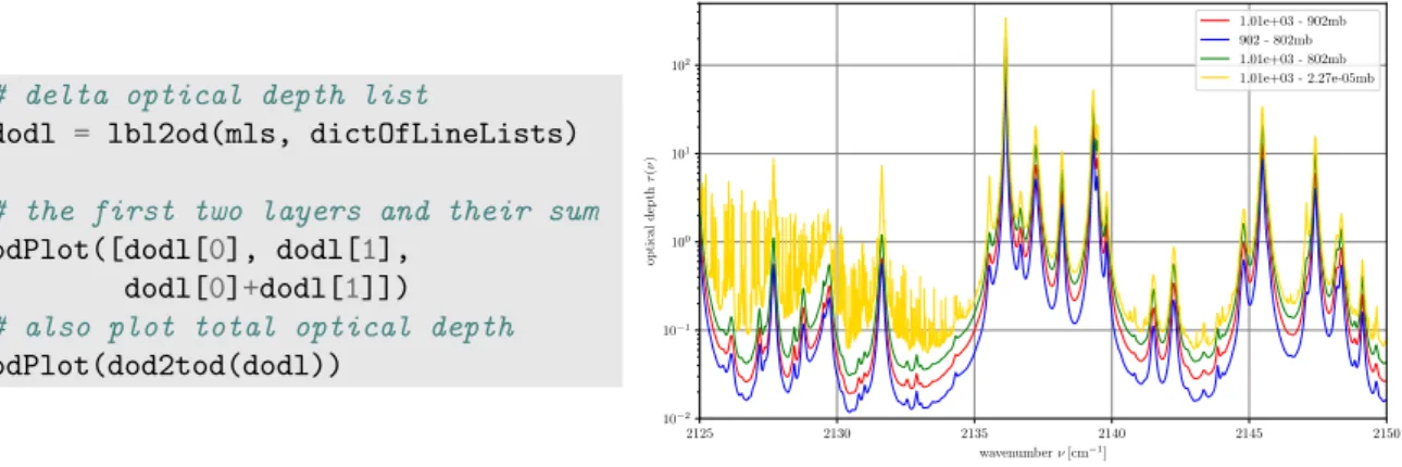
The optical depths instances can be combined by addition or subtraction, e.g., the delta optical depths of the first (bottom) two layers can be added by dodList[0]+dodList[1](see Figure 5).
The main purpose of the__add__special method is to combine the optical depths from neighboring layers, but it can also be used to sum the optical depths of different molecules in one layer.Version May 3, 2019 submitted toAtmosphere 12 of 26
# delta optical depth list
dodl = lbl2od(mls, dictOfLineLists) # the first two layers and their sum odPlot([dodl[0], dodl[1],
dodl[0]+dodl[1]]) # also plot total optical depth odPlot(dod2tod(dodl)) 2125 2130 2135 2140 2145 2150 wavenumberν[cm−1] 10−2 10−1 100 101 102 optical depth τ ( ν ) 1.01e+03 - 902mb 902 - 802mb 1.01e+03 - 802mb 1.01e+03 - 2.27e-05mb
Figure 5. Computing and combining optical depths.
thereof, or a dictionary of (lists of)xsArray’s. Figure4demonstrates the combined use of theatlas 365
andxsPlotfunctions exploiting Matplotlib’s functiontwinxto share the common wavenumber axis. 366
The functionsxsInfoandxsSavecan be used with a single cross section array, a list of cross sections, 367
or a dictionary of lists to summarize the cross sections’ properties or to write the data to file(s); Reading 368
cross section data from file(s) is possible with thexsReadfunction. 369
3.2.4. Absorption Coefficients 370
Given cross sections of some molecules on a set ofp,Tlevels along with the atmospheric data, in 371
particular the molecular number densities, the absorption coefficient (6) for all levels are generated 372
with acList = xs2ac (mls, xssDict). The list contains a spectrum for each atmosphericp,Tlevel, 373
where each spectrum is stored in a subclassed NumPy array:type(acList[0]) → acArraysimilar 374
to the cross sections, i.e. with attributes stored as, e.g.,ac.xandac.zfor the wavenumber range 375
and altitude, respectively. Note that the number of levels in the atmospheric data set (heremls) and 376
the lengths of the cross section lists in thexssDictdictionary has to be identical. Furthermore, all 377
molecules with cross section data must be contained in the atmospheric data (but there can be some 378
“unused” molecules in the atmospheric data set). 379
The absorption coefficients can be plotted with the standard Matplotlib functions, but Py4CAtS 380
also has a function to make this easier: acPlot(acList). The function acInfo(acList) prints 381
essential information about the absorption coefficients (Actually it is a loop calling the corresponding 382
infomethod ofacArray, i.e.for ac in acList: ac.info()). 383
The data can be saved to file (tabular-ascii) with the standard NumPysavetxt or Py4CAtS’ 384
awritefunction. TheacSavefunction automatically saves the absorption coefficients along with the 385
atmospheric data, and theacReadfunction allows to read the data (incl. the associated atmosphere) 386
back from file, e.g. absCo = acRead(acFile). Both acSave and acReadalso support HITRAN 387
formatted files or Python/NumPy’s internal pickle format. 388
3.2.5. Optical Depths 389
The next step is to integrate the absorption coefficients along the (vertical) path through the 390
atmosphere using the functionac2dod(seeIn[4]in Fig.3). Similar to cross sections and absorption 391
coefficients this returns a list of(nLevels-1)subclassed NumPy arraysodArray, where each list 392
member is essentially the delta / differential / layer optical depth spectrum along with its attributes 393
lower and upper altitudes, pressures, and temperatures (and the wavenumber interval, too). 394
The optical depths instances can be combined by addition or subtraction, e.g. the delta optical 395
depths of the first (bottom) two layers can be added by dodList[0]+dodList[1] (see Fig.5). The 396
main purpose of the__add__special method is to combine the optical depths from neighboring layers, 397
but it can also be used to sum the optical depths of different molecules in one layer. 398
Figure 5. Computing and combining optical depths.
Please note that theac2dodfunction (and thexs2dod,lbl2od, . . . function discussed below) only return delta optical depths (dod), further functions can be used to convert to cumulative or total optical depth. Summation of all layer optical depths with thedod2todfunction delivers the total optical depth anddod2codreturns the (ac)cumulated optical depth. By default, the accumulation is starting with the very first layer (usually at BoA) and the very last element of the generated list should be the total optical depth, whereascod = dod2cod(dodList,True)starts accumulating with the very last layer and the very firstcod[0]corresponds to the total optical depth.
A quick-look of optical depth(s) can be generated with theodPlotfunction, and the data (incl. the attributes) can be saved to file usingodSaveusing ASCII, netcdf, or pickle format. Later, the optical depth data can be read from file into a (new) IPython session withoDepth = odRead (odFile).
TheoDepthOnefunction returns the distances1from the (uplooking or downlooking) observer to the point, where the optical depth is one,τ(ν,s1) =1.0, corresponding to a transmission that has decreased toT = 1/e. This distance should roughly correspond to the location of the weighting
function maximum. 3.2.6. Weighting Functions
wgtFct = ac2wf(acList[, angle, zObs]) computes weighting functions according to Equation (13) for an observer at altitudezObslooking in directionangle(default 180◦) and returns a subclassed 2D NumPy array of typewfArray(withwgtFct.shape = (len(vGrid), len(sGrid))). By default, the observer is assumed to be at ToA or BoA for viewing angles larger or smaller than 90◦. The attributes define the wavenumber interval, path distance gridsGrid(relative to the observer (in cm), i.e., from ToA to BoA in case of a downlooking nadir view), observer altitude, and viewing angle. Optionallyac2wfalso allows the treatment of finite field-of-view effects with an extra argumentFoVto set the type and width (HWHM, in degree) (e.g.,FoV=’Gauss 7.5’).
Alternatively, given the delta/layer optical depths the weighting functions can be approximated by finite differencing using the dod2wf(dodList,zObs,angle) function, but starting from the absorption coefficient is much more reliable. For weighting functions of a horizontal path (zenith angle θ=90◦) see the first remark in Section4.2.
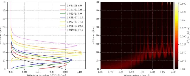
The functionwfSave(wgtFct, ...)andwfRead(wfFile, ...)can be used to save and read the data, andwfPlot(wgtFct[, wavenumber, ...])provides a simple visualization tool. If (a) specific wavenumber(s) are given, a 2D plot is presented, otherwise a contour plot is generated. An example of weighting functions for microwave temperature sounding in the region of the oxygen rotation band is given in Figure6.
AtmosphereVersion May 3, 2019 submitted to2019,10, 262 Atmosphere 14 of 2613 of 26
Figure 6.Combination of wfPlot. The labels in the left plot correspond to the central wavenumbers (in cm−1) for each of the seven SSM/T channels shown in Fig. 7.13 of Liou [2]. The second number
indicates the altitude grid point (in km) next to the maximum. This example has been generated with
sas = atmRead(’/data/atmos/50/subarcticSummer.xy’, zToA=80)
dll = higstract(’/data/hitran/2000/lines’,(0,10), ’main’); del dll[’CO’] acList = lbl2ac(sas, dll, (1.65,2))
wgtFct = ac2wf(acList, 180)
ssmtFreqs=array([50.5, 53.2, 54.35, 54.9, 58.825, 59.4, 58.4,])*1e9/c subplot(121); wfPlot(wgtFct, wavenumber=ssmtFreqs)
subplot(122); wfPlot(wgtFct, nLevels=50)
Note that theac2dodfunction (and thexs2dod,lbl2od, . . . function discussed below) only return 399
delta optical depths (dod), further functions can be used to convert to cumulative or total optical depth. 400
Summation of all layer optical depths with thedod2todfunction delivers the total optical depth and 401
dod2codreturns the (ac)cumulated optical depth. By default, the accumulation is starting with the 402
very first layer (usually at BoA) and the very last element of the generated list should be the total 403
optical depth, whereas cod = dod2cod(dodList,True) starts accumulating with the very last layer 404
and the very firstcod[0]corresponds to the total optical depth. 405
A quick-look of optical depth(s) can be generated with theodPlotfunction, and the data (incl. the 406
attributes) can be saved to file usingodSaveusing ASCII, netcdf or pickle format. Later on, the optical 407
depth data can be read from file into a (new) IPython session with oDepth = odRead (odFile). 408
TheoDepthOnefunction returns the distances1from the (uplooking or downlooking) observer
409
to the point, where the optical depth is one,τ(ν,s1) =1.0, corresponding to a transmission that has
410
decreased toT = 1/e. This distance should roughly correspond to the location of the weighting 411
function maximum. 412
3.2.6. Weighting Functions 413
wgtFct = ac2wf(acList[, angle, zObs]) computes weighting functions according to Eq. (13) 414
for an observer at altitudezObslooking in directionangle(default 180◦) and returns a subclassed 2D 415
NumPy array of typewfArray(withwgtFct.shape = (len(vGrid), len(sGrid))). By default the 416
observer is assumed to be at ToA or BoA for viewing angles larger or smaller than 90◦. The attributes 417
define the wavenumber interval, path distance gridsGrid(relative to the observer (in cm), i.e. from 418
ToA to BoA in case of a downlooking nadir view), observer altitude, and viewing angle. Optionally 419
ac2wfalso allows to treat finite field-of-view effects with an extra argumentFoVto set the type and 420
width (HWHM, in degree) (e.g.FoV=’Gauss 7.5’). 421
Alternatively, given the delta/layer optical depths the weighting functions can be approximated 422
by finite differencing using the dod2wf(dodList,zObs,angle) function, but starting from the 423
Figure 6.Combination of wfPlot. The labels in the left plot correspond to the central wavenumbers (in cm−1) for each of the seven SSM/T channels shown in Fig. 7.13 of Liou [2]. The second number
indicates the altitude grid point (in km) next to the maximum. This example has been generated with
sas = atmRead(’/data/atmos/50/subarcticSummer.xy’, zToA=80)
dll = higstract(’/data/hitran/2000/lines’,(0,10), ’main’); del dll[’CO’] acList = lbl2ac(sas, dll, (1.65,2))
wgtFct = ac2wf(acList, 180)
ssmtFreqs=array([50.5, 53.2, 54.35, 54.9, 58.825, 59.4, 58.4,])*1e9/c subplot(121); wfPlot(wgtFct, wavenumber=ssmtFreqs)
subplot(122); wfPlot(wgtFct, nLevels=50)
.
3.2.7. Radiance/Intensity
Thedod2rifunction evaluates the Schwarzschild integral (9) and returns the radiance or intensity, again a subclassed NumPy arrayriArraywith attributes for wavenumber interval, altitude, pressure, and temperature minimum/maximum, observer zenith angle, and background temperature, see the last block in Figure3. Without optional arguments, the radiance seen by an uplooking observer at the surface (BoA) is computed, whereasdod2ri (dodList, 180.0, mls[’T’][0])gives the radiance for a nadir-viewing observer looking down from ToA with an angle of 180.0◦(relative to the zenith angle) to Earth; the third argument specifies the surface temperatureTb(here the BoA temperature of the midlatitude summer (mls) atmosphere) that is used to evaluate a Planck background contribution in (9) withIb(ν) =B(ν,Tb).
Please note thatdod2ridoes not have any argument to specify the observer altitude, i.e., it computes the radiance at BoA or ToA for an angle smaller or larger than 90◦(a horizontal path with angle 90◦ is not implemented). If you want to model the radiance, say, for an airborne observer downlooking from 10 km and have a list of layer optical depths for an atmosphere with a uniform altitude grid of 1 km (hence layer thickness 1 km), supply a list of the first ten optical depths only, i.e., dod2ri(dodList[:10],180). (See also the remark on limitations in Section4.6.)
A further Boolean optional argument can be given to switch to the “B exponential-in τ” approximation instead of the default “B linear-inτ”, see Section2.2.2.
To plot and save the radiance spectrum (along with the wavenumber grid) in a file use the riPlotand riSavefunctions, respectively. To convolve the radiance spectrum I with a spectral response function according to (12), a special methodconvolvehas been implemented, e.g.,radBox1 = radiance.convolve()uses the default “box” with a half width 1.0 cm−1. Likewise,radGauss2
= radiance.convolve(2.0,’G’)uses a Gaussian response function with HWHM 2.0 cm−1. The
convolvespecial method is also available for theodArrayandwfArrayclasses (in the first case the convolution operates on the corresponding transmission).
3.2.8. Shortcuts
If some of the intermediate quantities are not required, it is possible to go directly from line and atmospheric data to optical depths usingdodList = lbl2od (mls, llDict). Likewise, cross sections and absorption coefficients can be bypassed with thelbl2acandxs2dodfunctions. Please note that lbl2acandlbl2od“inherit” most options accepted bylbl2xsorxs2ac.
4. Discussion
4.1. Selection of Spectral Range, Contributions from Line Wings
To compute cross sections, absorption coefficients, and optical depths for some spectral range νlo. . .νhi, all lines in an extended spectral rangeνlo−δ. . .νhi+δshould be considered, whereδis typically some wavenumbers ( cm−1). However, unless specified as fourth optional argumentxLimits of thelbl2xsfunction or as option-xof the command line scriptlbl2xs.py(and similarly for the lbl2acandlbl2odfunctions), the cross sections, absorption coefficients, and optical depths returned by Py4CAtS are computed on a uniform grid in the interval[νfirst,νlast]where the lower and upper limits correspond to the position of the very first and last line returned byhigstract. As thehigstract andlbl2xsscripts are completely independent, this extension is not done automatically. The impact of line wing contributions on cross sections is demonstrated in Figure7.
10 15 20 25 position ˆν[cm−1] 10−33 10−31 10−29 10−27 10−25 10−23 10−21 10−19 Strength S [cm − 1/ (molec . cm − 2)] Hitran 2008 — H2O 228 lines in 6 – 26cm−1 74 lines in 14 – 19 cm−1 43 lines in 15 – 18 cm−1 17 lines in 16 – 17 cm−1 16.0 16.2 16.4 16.6 16.8 17.0 wavenumberν[cm−1] 10−23 10−22 cross section k ( ν ) [cm 2/ molec] p=1 atm andT=296 K 228 lines in 6 – 26cm−1 74 lines in 14 – 19 cm−1 43 lines in 15 – 18 cm−1 17 lines in 16 – 17 cm−1
Figure 7.Impact of line wings on H2O cross section in the ODIN [83] 501 GHz channel. A series of
cross sections has been computed taking into account more and more lines to the left and right of the 16 to 17 cm−1window.
4.2. Optical Depths, Transmissions, and Weighting Functions for a Horizontal View
The functionsac2dodorlbl2oddo not have an angle as argument, so the optical depth returned is always the vertical optical depth through the atmosphere. If transmission (or weighting functions) for a horizontal path (i.e., zenith angle 90◦, hence a homogeneous atmosphere) are needed, the transmission T(ν,s) =exp(−α(ν)l)can be readily evaluated as a function of path lengthlgiven an appropriate
absorption coefficientα. Likewise, the weighting functions are easily computed according to (13) as the product of transmissionT(ν,s)times the absorption coefficientαfor some lengthsl.
4.3. Arbitrary Observer Positions
An observer “inside” a layer, i.e., with the observer altitude different from any atmospheric altitude grid point, is not supported by Py4CAtS. However, if one needs an observer at a specific altitude (e.g., 3.14159 km), one can interpolate the atmospheric profiles to a new grid including this point and proceed as usual.
![Figure 7. Impact of line wings on H 2 O cross section in the ODIN [83] 501 GHz channel](https://thumb-us.123doks.com/thumbv2/123dok_us/10115818.2912134/15.892.124.772.527.790/figure-impact-line-wings-cross-section-odin-channel.webp)