Portfolio optimisation models

(1)

Cristiano Arbex Valle

A thesis submitted for the degree of Doctor of Philosophy

School of Information Systems, Computing and Mathematics, Brunel University

(2)

Abstract

In this thesis we consider three different problems in the domain of portfolio optimisation. The first problem we consider is that of selecting an Absolute Return Portfolio (ARP). ARPs are usually seen as financial portfolios that aim to produce a good return regardless of how the underlying market performs, but our literature review shows that there is little agreement on what constitutes an ARP. We present a clear definition via a three-stage mixed-integer zero-one program for the problem of selecting an ARP.

The second problem considered is that of designing a Market Neutral Portfolio (MNP). MNPs are generally defined as financial portfolios that (ideally) exhibit performance in-dependent from that of an underlying market, but, once again, the existing literature is very fragmented. We consider the problem of constructing a MNP as a mixed-integer non-linear program (MINLP) which minimises the absolute value of the correlation between portfolio return and underlying benchmark return.

The third problem is related to Exchange-Traded Funds (ETFs). ETFs are funds traded on the open market which typically have their performance tied to a benchmark index. They are composed of a basket of assets; most attempt to reproduce the returns of an index, but a growing number try to achieve a multiple of the benchmark return, such as two times or the negative of the return. We present a detailed performance study of the current ETF market and we find, among other conclusions, constant underperformance among ETFs that aim to do more than simply track an index. We present a MINLP for the problem of selecting the basket of assets that compose an ETF, which, to the best of our knowledge, is the first in the literature.

For all three models we present extensive computational results for portfolios derived from universes defined by S&P international equity indices with up to 1200 stocks. We use CPLEX to solve the ARP problem and the software package Minotaur for both our MINLPs for MNP and an ETF.

(3)

4 Market neutral portfolios 64 4.1 Introduction . . . 64 4.2 Problem formulation . . . 65 4.2.1 Overview . . . 65 4.2.2 Notation . . . 65 4.2.3 Constraints . . . 67 4.2.4 Objective function . . . 68 4.2.5 Other constraints . . . 69 4.2.6 Zero-beta approach . . . 71 4.3 Computational results . . . 73 4.3.1 Minotaur . . . 73

4.3.3 Results, in-sample. . . 74

4.3.4 Results, out-of-sample . . . 76

4.3.5 Comparison with the zero-beta portfolio . . . 77

4.3.6 Comparison with market neutral S&P 500 funds . . . 79

4.3.7 Variations . . . 80

4.4 Discussions . . . 82

4.4.1 Choice of regression for the ARP model. . . 82

4.4.2 Pearson correlation coefficient . . . 82

4.4.3 Alternative approaches to MNP . . . 83

4.5 Conclusions . . . 84

5 Exchange-traded funds: a survey and performance analysis 86 5.1 Introduction . . . 86

5.2 ETF construction and literature review . . . 87

(5)

5.2.2 Regulatory concerns . . . 89

5.2.3 Literature review . . . 90

5.3 ETF survey . . . 92

5.4 ETF performance . . . 99

5.4.1 Underperformance in mean return . . . 101

5.4.2 Underperformance in volatility. . . 104

5.5 Summary and Conclusions . . . 107

6 An optimisation approach to constructing an exchange-traded fund 109 6.1 Introduction . . . 109 6.2 Problem formulation . . . 110 6.2.1 Notation . . . 110 6.2.2 Constraints . . . 112 6.2.3 Objective function . . . 113 6.2.4 Long/short fix . . . 114 6.3 Computational results . . . 114

6.3.2 Results, inverse ETFs . . . 115

6.3.3 Results, leveraged ETFs . . . 116

6.3.4 Varying h and α . . . 116

6.3.5 Results with transaction cost . . . 118

6.3.6 Results with restrictions on asset holdings . . . 119

6.4 Results, index tracking (L= 1) . . . 121

6.4.1 Artificial index . . . 121 6.4.2 Real index . . . 122 6.5 Conclusions . . . 123 7 Conclusions 125 7.1 Summary . . . 125 7.2 Contribution to knowledge . . . 127 7.3 Future research . . . 127 References 129

(6)

List of Figures

2.1 Efficient Frontier for the FTSE100. . . 6

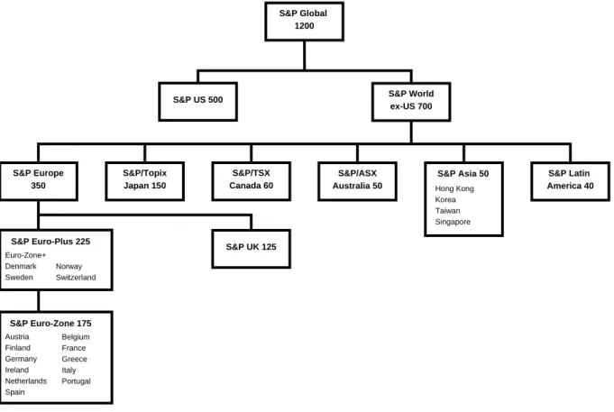
3.1 The structure of the S&P Global 1200 index, its components and the na-tions covered . . . 34

3.2 Out-of-sample portfolio and index value, S&P Global 1200, ARP-RT,H = 26 39

3.3 Varying K for the S&P Global 1200 . . . 56

3.4 ARP-RT, our approach compared with the 1/N portfolio . . . 58

5.1 Cumulative number of ETFs over time . . . 93

5.2 Single market equity ETFs: the top 20 countries by market value, showing percentage of total by market value and number of ETFs . . . 98

5.3 Multi-market equity ETFs: the top 20 indices by market value, showing percentage of total by market value and number of ETFs . . . 98

5.4 Commodity ETFs: the top 10 commodity or commodity indices by market value, showing percentage of total by market value and number of ETFs . 99

5.5 A comparison of ETF mean return with that of its benchmark. The mean is calculated over all available data . . . 102

5.6 A comparison of ETF volatility with that of its benchmark. Volatility is calculated over all available data. . . 105

(7)

List of Tables

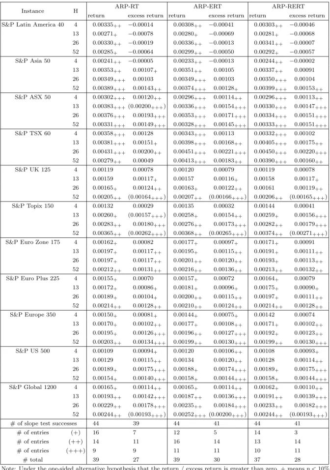
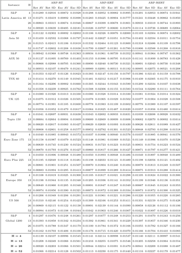
3.1 Out-of-sample returns and excess returns for each model . . . 37

3.2 Summary table for the slope test at varying significance levels . . . 40

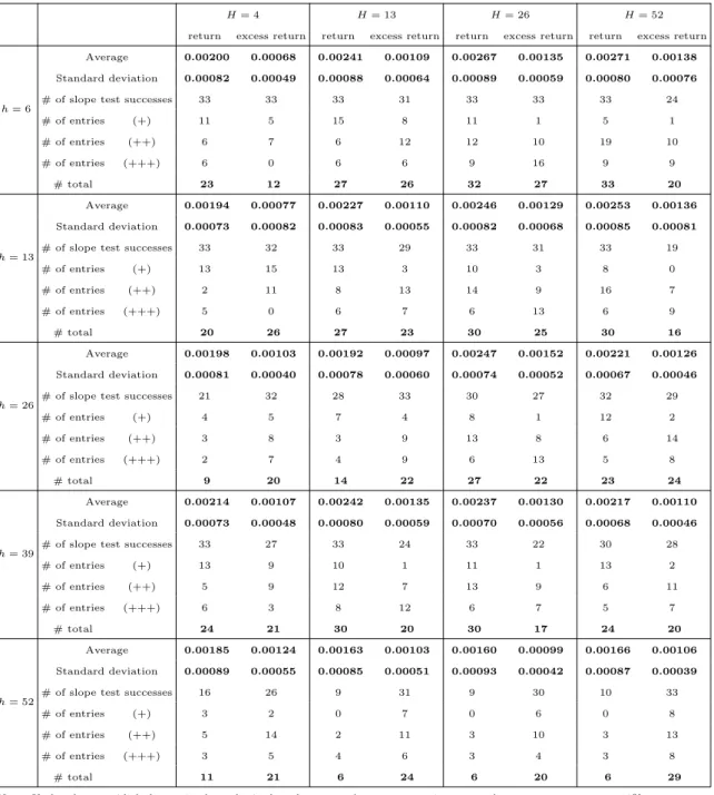
3.3 Average return and excess return for each choice of h and H . . . 41

3.4 Sharpe ratios . . . 43

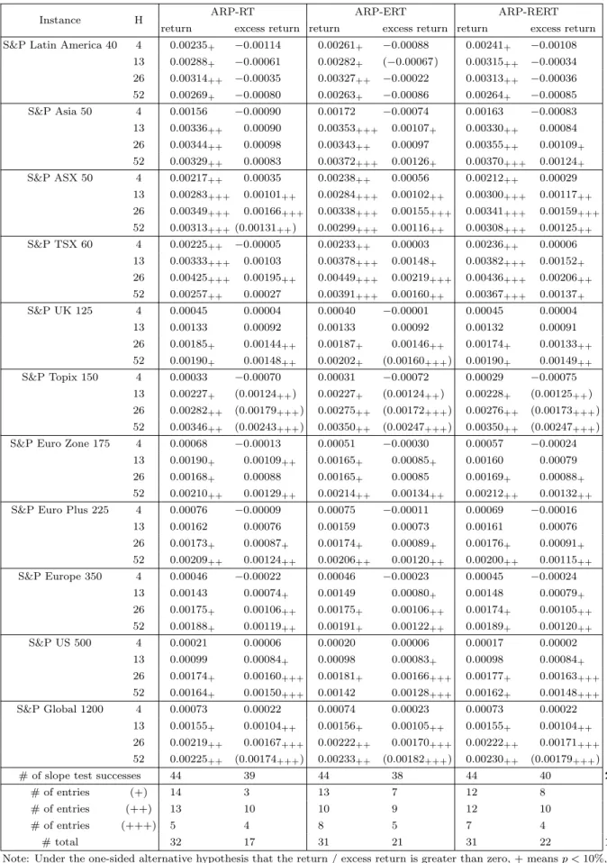
3.5 Out-of-sample returns and excess returns for each model, transaction cost case . . . 44

3.6 Sharpe ratios, transaction cost case . . . 46

3.7 Regression against time, p-value count . . . 47

3.8 Probability of Type II errors and p-values . . . 49

3.9 95% prediction interval counts . . . 50

3.10 Average mean return and standard deviation in return, averaged over all rebalances . . . 52

3.11 Prediction interval counts . . . 53

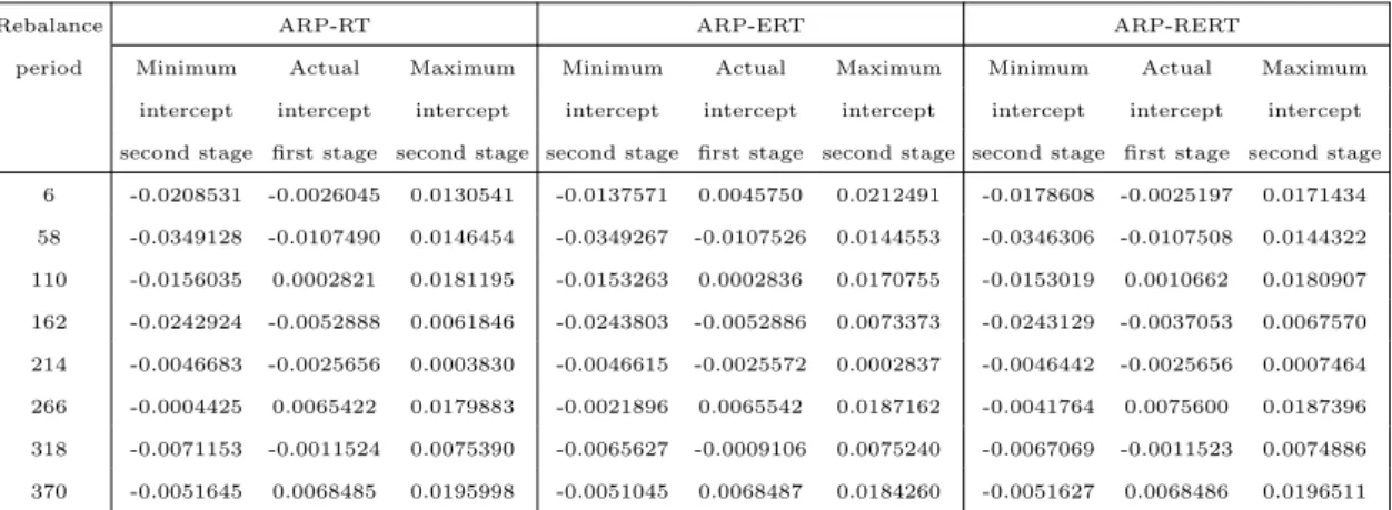
3.12 Intercept values, S&P Global 1200,H = 52 . . . 54

3.13 Sharpe ratios, 1/N portfolio . . . 59

3.14 Sharpe ratios comparison . . . 60

4.1 Summary of in-sample results . . . 75

4.2 Number of optimal solutions found . . . 76

4.3 Summary of out-of-sample results . . . 77

4.4 Comparison with the zero-beta model . . . 78

4.5 Comparison with market neutral S&P 500 funds . . . 79

4.6 In-sample summary statistics, different variations . . . 81

4.7 Out-of-sample summary statistics, different variations . . . 81

5.1 Papers dealing with the performance of ETFs . . . 90

5.2 ETF summary by number within each major and sub-classification and performance type . . . 94

5.3 Number of active ETFs by year of introduction and category . . . 95

5.4 ETF market value (MV) summary . . . 96

(8)

5.6 Two regressions to decompose the underperformance of an ETF in terms

of the properties of the ETF . . . 104

5.7 Regression to explain the difference between the volatility of an ETF and that of its benchmark in terms of the properties of the ETF . . . 106

5.8 Regressions looking at a decomposition of the difference between the volatil-ity of an ETF and that of its benchmark in terms of the properties of the ETF . . . 106

6.1 Tracking errors for the 150/50 case with L=−1 . . . 116

6.2 Tracking errors for the 150/50 case with L= 2 . . . 117

6.3 Average values for all instances with α= 0.5 . . . 117

6.4 Average values for all instances with h= 52 . . . 118

6.5 Tracking errors with transaction cost and L=−1 . . . 119

6.6 Tracking errors with transaction cost and L= 2 . . . 119

6.7 Tracking errors with asset limits,L=−1 . . . 120

6.8 Tracking errors with asset limits,L= 2 . . . 120

6.9 Artificial index, Minotaur versus PH . . . 122

(9)

Chapter 1 Introduction

1.1 Introduction

Ever since the pioneering work of Markowitz (1952), optimisation has been at the centre of work concerned with deciding the composition of financial portfolios. As such, both practitioners and academic researchers have been willing to trade off the disadvantages of optimisation (multiple optimal solutions, solution sensitivity) for its advantages (clear modelling framework, computational efficiency, algorithmic decision making).

The most popular portfolio optimisation problem is that of minimising risk for a given target expected return, or, conversely, maximising expected return while constraining risk. Different approaches measure risk differently, examples of different risk measures are variance of returns, CVar (Conditional Value at Risk, Rockafellar & Uryasev (2000)) and Sortino ratio (Sortino & van der Meer (1991)). Another popular portfolio optimi-sation problem is that of index tracking, where the concern is to reproduce (track) the performance of a financial index. Once again, there are different ways to measure tracking performance and hence there are different (and sometimes non-comparable) models for this purpose.

In short, different types of portfolios require different mathematical models, and, even for portfolios intended for the same purpose, the model to use is not uniquely defined. In this thesis we examine three portfolio optimisation problems that are not clearly defined in the present literature. We introduce optimisation models for the problems of selecting an Absolute Return Portfolio (ARP), a Market Neutral Portfolio (MNP) and the basket underlying an Exchange-Traded Fund (ETF).

ARPs are generally defined as financial portfolios that aim to produce good returns regardless of how the underlying market performs. However, our literature review shows that there is barely any agreement on what exactly defines a portfolio as an ARP. MNPs are defined as financial portfolios that (ideally) exhibit performance independent from

(10)

that of an underlying market. Once again, there are numerous models and different ways to measure the independence of a MNP. Based on these definitions, both problems seem similar and, indeed, one can think of a portfolio that is independent from a benchmark as one which produces absolute returns irrespective of how the benchmark is performing. These problems are however different, and, in this thesis, we present clear and unique definitions and we introduce optimisation models for both of them.

ETFs, on the other hand, are not per se a portfolio model. They are funds that are traded on the open market and that usually have their expected performance tied to a benchmark index. ETFs are composed of a basket of assets held by the ETF creator and shares that are issued and traded in the open market. An ETF share entitles its holder to a portion of the underlying basket. Most ETFs are index trackers, however, some seek to achieve a multiple of benchmark return. For example, some ETFs aim to achieve the negative of index return, while others seek to achieve twice index return. The former are called inverse ETFs and the latter are known as leveraged ETFs. In this thesis we also examine the optimisation problem of defining an ETF basket of assets, a non-trivial problem especially for leveraged and inverse ETFs.

1.2 Thesis outline

The structure of this thesis is as follows. In Chapter 2 we present a literature survey of portfolio optimisation in general with special attention to ARPs, MNPs and ETFs. We start by summarising the history and context of portfolio optimisation theory. We then dedicate separate sections to the literature on each of the three main problems studied in this thesis.

In Chapter3 we consider the problem of selecting an ARP. We present a three-stage mixed-integer zero-one program for the problem that explicitly considers transaction costs associated with trading. The first two stages relate to a regression of portfolio return against time, whilst the third stage relates to minimising transaction costs. We extend our approach to the problem of designing portfolios with differing characteristics. Com-putational results are given for portfolios of eleven different problem instances derived from universes defined by S&P international equity indices.

In Chapter 4 we consider the problem of constructing a MNP. We formulate this problem as a mixed-integer nonlinear program (MINLP), minimising the absolute value of the correlation between portfolio return and index return. Our model is a flexible one that incorporates decisions as to both long and short positions in assets. Computational results, obtained using the software package Minotaur, are given for the same problem instances as in Chapter4. We also compare our approach against an alternative approach

(11)

based on minimising the absolute value of regression slope (the zero-beta approach). In Chapter5we present a survey of the current ETF market by collecting and analysing a large snapshot of 8192 ETFs, which compose the vast majority of the ETF market. We selected a subset of 822 ETFs to analyse more fully. Our performance analysis covers the period from January 1993 to September 2011 and statistically analyses these 822 ETFs, which have a total market value of US$1.81 trillion, using over 1.1m daily return observations. The accuracy with which ETFs replicate the behaviour of their benchmark is a mixed story; only 19% of ETFs reproduce both the mean return and the volatility of their benchmark within 1% p.a.. With respect to replicating benchmark volatility we found that most ETFs have higher volatility than their benchmarks.

Following the ETF survey performed in Chapter 5, we consider in Chapter 6 the problem of deciding the portfolio of assets that should underlie an ETF. We formulate this problem as a MINLP. We mostly consider ETFs which have positive leverage with respect to their benchmark index, as opposed to ETFs which simply attempt to track the benchmark performance, and ETFs which have negative leverage (inverse ETFs). Our formulation is a flexible one that incorporates decisions as to both long and short positions in assets, as well as including rebalancing and transaction costs. Computational results are given for problems for the same set of instances as used in Chapter 3. We also computationally compare our model to a previous model in the literature for index tracking.

Finally, in Chapter7 we summarise the main results of our research, highlighting the contribution to knowledge we have made, and suggest directions for future work.

(12)

Chapter 2 Literature review

In this chapter we present a brief historical overview of portfolio optimisation and discuss studies in the literature related to Absolute Return and Market Neutral portfolios. We also discuss work related to Exchange-Traded Funds.

2.1 History of portfolio theory

The foundations of Modern Portfolio Theory (MPT) date back to the 1950s thanks to a landmark article and subsequent book by Markowitz (1952, 1959). Prior to his work, assets were analysed individually in order to construct a portfolio. Markowitz proposed that portfolios should be selected based on overall (instead of individual) risk-return assessment. An important assumption of MPT is that investors are risk averse, meaning that given two portfolios that offer the same expected return, investors will choose the less risky one. Investing is a tradeoff between risk and return; investors will take increased risk only if compensated by higher expected returns. Following this assumption Markowitz formulated the portfolio problem as that of finding the weighting of assets that minimise risk given a target expected return. Risk is measured as variance of expected returns.

The important message of MPT is that assets should not be selected only on charac-teristics that are unique to the asset. Rather, investors have to consider how each asset relates to all other assets.

To present the basic Markowitz mean-variance portfolio model, we need to introduce some notation. Let:

(13)

N be the number of assets available, ¯

ri be the expected (average, mean) return (per time period) of asset i,

ρij be the correlation between the returns for assets iand j (−1≤ρij ≤+1),

si be the standard deviation in return for asset i,

σij be the covariance between returns for assets i and j (σij =ρijsisj), and

M be the desired expected return from the portfolio chosen.

Then the decision variables are:

ωi the proportion of the total investment associated with asset i(0≤ωi ≤1).

Observe that we imposed non-negativity (ωi), meaning we can only go long, that is,

buying and holding an asset in the hope that its price will rise. If we were to allow negative weights (soωi can be positive or negative), then we would be allowing shorting. Shorting

(or short selling) is when investors borrow a particular asset and sell it immediately in the market, in the hope that the asset price will fall, enabling them to buy the asset back later at a lower price and return it to the original lender.

Using the standard Markowitz mean-variance approach we have that the portfolio optimisation problem is:

minimise N X i=1 N X j=1 ωiωjσij (2.1) subject to N X i=1 ωir¯i =M, (2.2) N X i=1 ωi = 1, (2.3) 0≤ωi ≤1, i= 1, . . . , N. (2.4)

Here in Equation (2.1) we minimise the total variance (risk) associated with the portfolio. Equation (2.2) ensures that the portfolio has an expected return of M. Equation (2.3) ensures that the proportions sum to one, so that all available cash is invested in assets.

This formulation is a nonlinear programming problem. Usually nonlinear problems are difficult to solve, however in this case, since the objective is quadratic and [σij] is positive

semidefinite (a property of covariance matrices), computationally effective algorithms exist so that in practice the above model can be solved with little difficulty.

(14)

The point of the above optimisation problem is to construct an efficient frontier, a smooth non-decreasing curve that gives the best possible tradeoff of risk against return, i.e. the curve represents the set of Pareto-optimal (non-dominated) portfolios.

Beasley (2013) gives one such efficient frontier, shown in Figure 2.1, for assets drawn from the UK Financial Times Stocks Exchange (FTSE) index of top 100 companies. Note how this nice smooth continuous curve runs from the minimum variance portfolio to the maximum return/maximum risk portfolio. Here we can choose to hold any of the portfolios on this efficient frontier. For this particular data set the minimum variance portfolio contained 30 out of the 100 assets.

Figure 2.1: Efficient Frontier for the FTSE100

Based on Markowitz’ mean-variance model,Treynor(1961),Sharpe(1964) andLintner

(1965) independently introduced the Capital Asset Pricing Model (CAPM). CAPM says that the expected return of an asset or portfolio equals the return on a risk-free asset plus a risk premium. If an asset is to be added to an already diversified portfolio, CAPM determines a theoretically appropriate rate of return that compensates the investor for taking the risk premium associated with that asset. CAPM assumes that each individual asset in a portfolio entails specific risk, but, through diversification, an investor’s net exposure can be reduced to the systematic risk of the market portfolio.

The general idea behind CAPM is that investors need to be compensated in two ways: time value of money and risk. The time value of money is represented by the risk-free rate (which we denote as rf), which means how much return an investor would expect

from an absolutely risk-free investment over a given period of time. A rational investor that decides to take a risky investment expects at least to exceed the risk-free rate.

The other input to CAPM is the amount of compensation an investor needs for taking additional risk. This is calculated by taking the asset’s sensitivity to non-diversifiable

(15)

(specific) risk, often represented by the quantityβin the financial industry, and comparing the asset returns to the market premium (return over a risk-free investment). Given observed market returns rm and asset a returnsra,βa is calculated as:

βa =

σma

σ2

m

, (2.5)

where σma is the covariance between asset returns ra and market returns rm, and σm2 is

the variance of market returns rm. Given expected market return ¯rm, in order to decide

whether an asset should be added to a portfolio we have to apply, according to CAPM, the formula:

¯

ra=rf +βa(¯rm−rf) (2.6)

where asset a should be included in a portfolio only if its expected returns exceed ¯ra.

An important assumption of CAPM is that asset prices move together because of one factor: the common movements of markets. The simplicity of CAPM led to the development of Arbitrage Pricing Theory (APT), first proposed by Ross (1976). APT considers that the expected return of an asset can be modelled as a linear function of various macroeconomic factors or theoretical market indices, where sensitivity to changes in each factor is represented by a factor-specific β coefficient. These models are usually referred to as factor models (see Wilmott (1998); Alexander(2001); Elton et al. (2007)). The standard form of a factor model can be written as

¯ ra = m X j=1 βajfj +a (2.7)

whereβaj are factor-specific sensitivities,m is the number of factors anda is the portion

of the return on asset a not related to any of them factors.

The success of factor models in predicting returns depends on both the choice of the factors (fj) and the method for estimating factor sensitivities (βaj). Factors may be

chosen according to economics (interest rates, inflation, etc.), finance (market indices, yield curves, exchange rates, etc.), fundamentals (book-to-market ratios, dividend yields, etc.) or statistics (factor analysis, principal component analysis, etc.). Sensitivities can be estimated using cross-sectional regression, time series techniques or eigenvalue methods.

The most popular factor model is the Fama-French three-factor model, designed by

Fama & French (1993) to describe asset returns. Fama and French observed that two classes of assets have tended to outperform the market: small caps and assets with a high book-to-market ratio. They expanded CAPM to include portfolio exposure to these two classes. According to the Fama-French three-factor model, asset return is explained according to the formula:

(16)

¯

ra=rf +βa1(¯rm−rf) +βa2 SMB +βa3 HML +a (2.8)

where SMB stands for “Small (market capitalisation) Minus Big” and HML stands for “High (book-to-market ratio) Minus Low”. Here βa1 is analogous to the classical βa

(given in Equation (2.5)) but not equal to it since there are now two additional factors.

2.2 Discussion on portfolio models

In the Markowitz framework, the portfolio is decided so as to minimise risk, where risk is defined as the in-sample variance in portfolio return. Clearly, risk can be defined in different ways. For example, a downside risk framework would equate risk with portfolio return falling below a predefined target. In this case, the objective of our optimisation model would be changed.

In fact, minimising risk is one of many possible objectives when defining a portfolio optimisation model. Take, for instance, the problem of designing an index tracking port-folio, where the objective is to replicate the performance of an index such as the S&P500 or the FTSE100.

In order to achieve this, full replication (buying all assets in the proportions that they compose the index) is possible, albeit for larger indices it can be an expensive strategy in terms of transaction cost. For example, whenever an asset enters/leave the index, the entire fund must be rebalanced, and any new money invested in the fund must be spread across all assets to mirror the index. For these reasons it is common not to adopt full replication. In such cases it is necessary to solve an index tracking portfolio optimisation model where the number of assets that can be bought is restricted. The objective of this problem is to minimise the tracking error, defined as the average squared difference between the tracking portfolio return and the index return.

Tracking error, however, is not the only way to measure the success of an index tracking portfolio. An alternative view on the above problem relates to regression. Suppose we perform a linear regression of the return from the tracking portfolio against the return of the index, i.e. the regression rt = α+βRt, where rt and Rt are the portfolio and index

returns at time t. If we are looking for an index tracking portfolio then clearly we want an interceptα = 0 and a slopeβ = 1. We can obtain αand β by using an ordinary least-squares regression (as in Canakgoz & Beasley(2009)), or, alternatively, by using quantile regression (Mezali & Beasley(2013)). The former looks for regression coefficients based on the least-squares mean regression line, while the latter uses coefficients based on median regression (the 50% quantile).

(17)

Recent work, other than that discussed above, dealing with index tracking can be found in Chen & Kwon (2012), Garcia et al. (2011), Guastaroba & Speranza (2012),

Krink et al. (2009), Maringer (2008), Ruiz-Torrubiano & Suarez (2009), van Montfort et al. (2008), and Wang et al.(2012).

Essentially, different types of portfolios require different mathematical models, and even for portfolios intended for the same purpose, the model to use is not uniquely defined, such as the index tracking problem discussed above. In this thesis, we concentrate on three problems which in our view are not well defined in the literature: the problems of selecting an absolute return portfolio, a market neutral portfolio and an asset basket for an exchange-traded fund. We review the literature on each of these problems in the next sections.

2.3 Absolute return portfolios

The reader should be aware that the term ‘Absolute Return Portfolio’ is not clearly defined, as noted previously for example by Waring & Siegel (2006). Differing authors interpret the phrase ‘Absolute Return’ differently, as will be seen in our discussion of the literature below.

2.3.1 Stochastic programming models

One strand relevant to ARPs that can be found in the literature relates to guaranteed return funds. They fall within the ARP category as they aim to achieve a minimum absolute return. Work that deals with guaranteed return funds is often based on stochastic programming or some other form of future scenario prediction. The minimum return will hence be guaranteed provided the future is one of the predicted scenarios.

Dert & Oldenkamp (2000) proposed a stochastic programming model for a single-period guaranteed return portfolio that may include European put and call options. In this work a casino effect is shown to exist when one chooses portfolios to maximise expected return subject to achieving a minimum level of return under all circumstances (scenarios). The casino effect arises where there are high probabilities of obtaining low returns and low probabilities of receiving high returns. Since investors may dislike casino solutions the authors enhance their model by adding chance constraints which require that the probabilities of achieving returns less than pre-specified levels should be small. Numeric testing is based on options from the Standard & Poor’s 500 index for 1997 with an investment horizon of 23 days. No details are given on the solution approach used.

(18)

Berkelaar et al. (2002) proposed an interior point approach based on primal-dual decomposition for a two-stage stochastic linear program. The work itself presents a general algorithm for this class of stochastic problems, but as an illustration their method is applied to a portfolio optimisation problem where an investor can invest in a money market account, a stock index and options on the index; moreover, a minimum return has to be guaranteed over a set of future scenarios. In their problem the portfolio (once constructed) can be rebalanced once (on a set date) before the end of the time horizon. The author mention, as advantages of their work, that the method proposed does not need a feasible starting solution and its computation time seems to grow linearly with the number of scenarios. Numeric testing is based on high liquidity options for the Standard & Poor’s 500 index for 1999. The number of scenarios considered is 50 for the rebalancing date and 100 for the time horizon. No computation time for this portfolio optimisation problem is given, however there is a computational time comparison for some other test problems where their algorithm shows a much better performance than its deterministic equivalent. See Berkelaar et al. (2005) for an extension of this work to multistage stochastic convex programs.

Another work that relies on stochastic programming to guarantee a minimum return is that presented by Dempster et al. (2007). They proposed a stochastic formulation to a complex multivariable problem where, after an initial investment in a closed end guarantee fund, the objective is to hedge the risks involved in order to avoid having to buy costly insurance to guarantee the minimum return. This problem requires long-term forecasting in multiple time periods for many investment classes. They proposed a dy-namic stochastic programming model to solve the problem. Stock prices are modelled using both standard geometric Brownian motion and geometric Brownian motion with Poisson jumps. Backtesting is presented for a 5 year period, from January 1999 to De-cember 2003. The model is compared to the Euro Stoxx 50 index. Given a minimum barrier which the portfolio must exceed over time, the model behaves quite well, the only period where it drops below the barrier is on the 11th of September 2001. The number of scenarios considered is either 7776 or 8192, depending on the tree structure used for different horizon backtests, but no computation times are given. See also Dempster et al.

(2006).

Herzog et al. (2007) applied sequential stochastic programming to an Asset Liabil-ity Management (ALM) problem that guarantees a minimal return on investments. The stochastic programming optimisation is resolved for every time interval on a new set of stochastic scenarios that is computed according to the latest conditional information. They show that such a technique approximates a continuous state dynamic programming algorithm and that, by using a sufficiently large number of scenarios, the difference

(19)

be-tween the exact solution and the approximation can be made arbitrarily small. They also argue that the most suitable risk measures for guaranteed return funds are shortfall risk measures. Hence, they define a penalty function relating to any shortfall below guaran-teed return. Their objective function is to maximise multi-period return while keeping the penalty function under a certain level as defined by a coefficient of risk aversion. The model also includes transaction costs. They presented a case study relating to a Swiss fund with quarterly data over the period 1988 to 2005 with up to 5000 scenarios.

Barro & Canestrelli(2010) proposed a multistage stochastic programming framework for a dynamic asset allocation problem which takes into account the conflicting objectives of a minimum guaranteed return and of an upside capture of asset returns. They argue that maximising the upside capture increases the total risk of the portfolio, thus they attempt to balance this by introducing a second goal where they try to minimise the shortfall with respect to the minimum guarantee level. To combine these two conflicting goals they formulate them in the framework of a double dynamic tracking error problem using asymmetric tracking measures, one for a risky benchmark and one for a minimum guaranteed benchmark. The objective is a combination of both tracking errors functions. They describe the uncertainty of future returns by using the concept of a scenario tree where each scenario is represented as a path from the origin to a leaf of the tree. An interesting feature of this model is the introduction of liquidity constraints which take into account the bid-ask spread. They also briefly discuss a second approach where the problem of minimum guaranteed return is tackled with the introduction of chance constraints. No numerical results are given.

2.3.2 Other models

There are also papers presented in the literature that (unlike those discussed above) do not use stochastic programming.

Nishiyama(2001) considered an absolute return strategy derived from multi-manager investment, a fund of funds (FoF) approach, in Japan. He argued that FoFs have tra-ditionally low correlation against the benchmark index and little impact from external changes, thus being absolute return strategies. He observes that nonlinear events occur frequently in the market, e.g. crashes, and that this phenomena should not be interpreted using traditional theory framework, which divides a portfolio risk in two: systematic (market) and unsystematic (specific) risk. He then proposes the use of the physics the-ory of Self-Organised Criticality (SOC) to find the point at which a system changes its behaviour or structure, for instance, from solid ice to liquid water. Unlike the melting case, where the control parameter is the temperature, a SOC reaches a critical state by its

(20)

intrinsic dynamics, e.g. the market reaches a critical state when it crashes and this is not due to a control parameter. To understand the dynamics he focused on the correlation matrix of nonlinear fluctuations in the market, where he looked into historical movement of asset correlation and assumed its behaviour would be ex-ante signals of a market crisis. He introduces a third risk category called group risk, which lies between systematic and unsystematic risk and accounts for the nonlinear type of market movements. He believes that minimising variance is not sufficient to measure risk, and he emphasises the impor-tance of correlation rather than variance. Simulated results over the period 1995-2000, so including the 1998 Russian crisis and the failure of Long-Term Capital Management, were presented.

Korn(2005) proposed a different approach for portfolio selection with a positive lower bound on the final wealth. The solution given consists of transforming the original problem into an equivalent unconstrained portfolio problem with a modified utility function that does not include the lower bound. Unlike the majority of work on guaranteed return funds, time is considered a continuous series instead of being divided into discrete intervals. As mentioned by the author, the unconstrained version is solved analytically via numerical methods, although no details are given on which numerical methods were used. After the problem is solved, the optimal final wealth is separated into a hedging term, needed to satisfy the requirement of a minimum final wealth, and a speculative term. The hedging term is a portfolio made up of put options and stocks. The speculative part could be calculated by computing the delta of the corresponding options. A few examples are given that demonstrate the relationship between stock investment and the growth or decay of total wealth, however, the deltas (speculative term) are not computed since they require lengthy expressions to be solved. No computational results are given for real world data. Stock prices are modelled using generalised geometric Brownian motion.

Amenc et al. (2008) proposed an approach based on a dynamic core-satellite portfo-lio. This technique, explained in detail in Amenc et al. (2004), consists of splitting the cash allocation into different portfolios. The core portfolio is mainly a low-risk portfolio that intends to respect the investor’s long-term risk return objectives, while the satellite portfolio provides access to upside potential by investing in more risky assets that are expected to outperform the benchmark. At discrete time intervals, the investor decides the proportion invested in each portfolio based on a minimum guaranteed value that is relative to the benchmark, e.g. 90% of an underlying index. The dynamic allocation pro-cess will systematically increase the exposure to the satellite portfolio when it does well with respect to the core, while controlling risks by shifting to the core when the satel-lite does poorly. They gave an example where the core is composed of Euro bonds and the satellite is an exchange-traded fund relating to the Euro Stoxx 50. They compared

(21)

their core-satellite approach with an active manager simulation, and showed that overall their dynamic core-satellite portfolio led to better results than a simulation of an actively managed portfolio built on largely accurate forecasts.

Lejeune(2011) considered an absolute return strategy derived from a long-only fund of funds approach which was formulated as a mixed-integer nonlinear programming problem. Portfolio variance is constrained to be below a given limit, this is ensured through a Value-at-Risk (VaR) constraint that limits the magnitude of the loss with a specified probability level over a certain period of time. In the model presented VaR takes the form of a prob-abilistic constraint. They estimate asset returns by using the Black-Litterman framework (Black & Litterman(1992)) which attempts to overcome problems of highly-concentrated input-sensitive portfolios. The model presented is computationally expensive and thus the probability constraint is approximated deterministically by a second-order cone con-straint which makes the problem convex for a wide range of probability distributions. They present a specialised nonlinear branch-and-bound algorithm which is implemented by an open source nonlinear solver. The branch-and-bound is compared to two other solvers in terms of computational performance over 12 different problem instances.

Zymler et al. (2011) proposed an approach based on combining robust optimisation with options, an approach they call insured robust portfolio optimisation. Robust optimi-sation (e.g. see Ben-Tal & Nemirovski (1998)) gives a guarantee provided data variation lies within a specified uncertainty set. They add another layer of guarantee to hedge against rare events which are not captured by a reasonably sized uncertainty set. They enrich the portfolio with specific derivative products to obtain a deterministic lower bound that essentially provides a barrier (insurance) such that the portfolio value cannot drop below the required level. They argue that enlarging the uncertainty set to cover extreme events (instead of adding the second layer of insurance) would lead to robust portfolios that are too conservative and could perform poorly under normal market conditions. The model they develop is a convex second-order cone program which is scalable in the number of stocks. Numeric results were given based on simulated data as well as historical data, where they observed that while the uninsured portfolio tends to have higher expected re-turns in normal market conditions, the proposed insured model shows clear advantages in terms of Sharpe ratios, expected returns and cumulative wealth when the markets behave abnormally.

2.4 Market neutral portfolios

The history of Market Neutral Portfolios traces back to the mid-1980s, when Morgan Stanley assembled a group of mathematicians, physicists and computer scientists to

(22)

de-velop trading programs whose intention was to take the intuition and trader’s “skill” out of arbitrage and replace it with disciplined, consistent filter rules. Among other things, this group identified pairs of securities that tended to move together. This marked the beginning of Pairs trading, which is the first known market neutral technique and it is generally assumed to be the ancestor of statistical arbitrage (see Gatev et al. (2006)).

Pairs trading works as follows. If two assets (sayP andQ) are in the same industry or have similar characteristics, one expects the two asset returns to track each other within a certain error. If Pt and Qt denote the corresponding price series which are historically

correlated, then we can model a system such as:

ln(Pt/Pt0) = Sln(Qt/Qt0) +t (2.9)

wheretis a stationary, or mean reverting, process, usually known ascointegration residual

and S is a constant equating ln(Pt/Pt0) with ln(Qt/Qt0). The model above suggests an investment strategy where, if t is sufficiently positive, we short S£ of asset Q for every

1£ invested in long positions of asset P. Conversely, if t is sufficiently negative, we go

short on P and long on Q. The portfolio is expected to oscillate near some statistical equilibrium, bringing tcloser to zero. This is usually called a mean-reversion strategy as

the investor bets that the prices will eventually revert to their historical trends. This is typically associated with market overreaction: assets are temporarily under or overpriced with respect to one or several reference securities (Lo & MacKinlay (1990)). See Pole

(2008) for a comprehensive review on statistical arbitrage and cointegration.

Pairs trading is considered market neutral as it provides a hedge against market risk. For example, if the whole market crashes, and the two assets plummet along with it, the trade should result in a gain on the short position and a loss on the long position, leaving the profit close to zero in spite of the large move. Note, however, that market neutral investing is not a single strategy; pairs trading is one possible technique to achieve market neutrality. For instance, an alternative strategy is known as delta neutral, where delta is defined as the sensitivity of an option value with respect to changes in the underlying asset’s price when all other variables remain unchanged. A delta neutral portfolio is one which tries to maintain its value unchanged when small changes occur in the value of the underlying securities. Such a portfolio typically contains options and their corresponding underlying securities such that positive delta components (namely, long call or short put options) and negative delta components (short call or long put options) offset. Work found in literature that study market neutral investments are summarised below.

Avellaneda & Lee(2010) define a market neutral portfolio as one that is uncorrelated with the market. They define the market as the combination of multiple factors, where they present a model to explain stock returns as composed of a systematic component

(23)

dependent on factors and an idiosyncratic (uncorrelated) component. They then regard a market neutral portfolio as one where the portfolio has zero exposure to these factors. To estimate the factors they use two different approaches. The first one is called the Principal Components Analysis (PCA) (see Jolliffe (1986)) which uses historical data to create an empirical correlation matrix. From this matrix they extract eigenvalues and rank them in decreasing order, where those that exceed a given percentage of the trace of the correlation matrix are considered significant. From the significant eigenvalues they form weighted “eigenportfolios”, which are the estimates of factors. In the second approach, they select a sufficiently diverse set of Exchange-Traded Funds (ETFs) and consider them as factors. Extensive computational results were given, where they noted that the performance of mean-reversion strategies appears to benefit from situations where most of the variance can be “explained” (with significant regression coefficients) by a relatively small number of factors. If the “true” number of factors needed to explain variance was very large then using only a few factors would not be enough to “defactor the returns”, so residuals would “contain” market information that the model is not able to detect. If, on the other hand, they used a large number of factors, the corresponding residuals would have small variance, and thus the opportunity of making money, especially in the presence of transaction costs, is diminished.

Baronyan et al. (2010) investigated different pairs trading strategies by combining 7 different policies of pairs selection with 2 trading methods, in a total of 14 strategies. Together the pairs are meant to be “market neutral” although, as is clear from the varying strategies proposed in Baronyan et al.(2010), there are many different measures that can be used to decide whether a pair is “market neutral” or not. Computational results were presented for pairs of stocks drawn from the Dow Jones 30 index, so 30₂ = 435 pairs. Yearly tests were performed fromN = 1999, . . . ,2006, where yearsN andN+ 1 comprise the training (in-sample) period, and year N + 2 comprises the testing (out-of-sample) period. Thus, the last test included the year of the global financial crisis. They compared the seven different strategies and found that in general all of them resulted in positive cumulative returns, especially in 2008. They argued that mispricings in pairs of similar stocks are more commonplace in a global crisis, thus allowing more trading possibilities to emerge in bad times.

Ganesan(2011) used a regression of individual stock returns against a number of fac-tors. He defines a market neutral portfolio as one whose exposure to factors is zero. He presents a single factor and a multi-factor model for describing the stocks expected re-turns. He adopted a Markowitz mean-variance approach to portfolio construction, where new constraints were added to transform the problem into that of finding a market neu-tral portfolio. Using geometrical subspace analysis he shows that any portfolio can be

(24)

decomposed as the sum of a market-neutral portfolio and a factor-exposure portfolio. Examples with three stocks were used to explain both the single factor and multi-factor approaches. An empirical study was performed comprising all U.S. stocks traded on New York and NASDAQ (about 2000 stocks) during the period from 1998 to 2010. The study results show that the performance of the market-neutral component depends on the cross-sectional variation of stock returns (called dispersion), while the performance of the factor component depends on the volatility of the overall stock market.

Kwan (1999) used a regression of stock returns against market returns and regarded a market neutral portfolio as one where the long portfolio weighted regression parame-ters relating to slope are equal to the equivalent short parameparame-ters. His model focused on accurately portraying institutional procedures for short selling (i.e. by including in the model all possible costs involved in short transactions) while adhering to the mean-variance framework. The portfolio is subject to a constraint where the weighted average of the long and short beta (slope) coefficients must be equal and the model’s objective is to maximise the Sharpe ratio (Sharpe(1966, 1975,1994)). The securities are doubled (to account for long and short) and ranked according to criteria that take into consideration how undervalued (overvalued) a particular asset is. The model is solved via an itera-tive procedure where securities are added one by one to the portfolio while maintaining feasibility. Computational results were given for one illustrative example involving 20 stocks from the Dow Jones Industrial index. The model is flexible enough to accommo-date different market outlooks by adjusting the weights between the market-neutral and market-sensitive components.

Ma et al.(2011) used a regression of individual stock returns against a number of fac-tors. In their regression different parameters applied depending upon the market regime (e.g. bull or bear market, where prices are increasing or decreasing respectively). They formulated a stochastic linear program to maximise portfolio return whilst constraining the portfolio factor exposure to lie within limits. The market neutral strategy is imple-mented by constructing and rebalancing the portfolio that has overall zero betas for all relevant risk factors and thus the return of the portfolio under such a strategy is uncor-related with the market risk factors. They used Bayesian information criteria to estimate the number of regimes. Three regimes were identified, where the third (apart from bull and bear) was a transitional market. A transition probability matrix between the three regimes is given, but no details are provided on how it was estimated. Computational results were given for one example involving nine sector ETFs over the period January 2005 to September 2009. The strategy is compared to a benchmark strategy which invests passively and equally among the nine sector ETFs. Their results show that, in general, the regime-dependent strategy outperforms the benchmark strategy. Their evaluation,

(25)

however, did not include a bear market situation.

Pai & Michel (2012) used a regression of stock return against market return and re-garded a market neutral portfolio as one where the portfolio weighted regression parame-ters relating to slope are nonlinearly constrained. They used a Markowitz mean-variance approach to portfolio construction with a nonlinear portfolio risk constraint. They argued that while the problem of constructing a basic market neutral portfolio could be modelled as a linear program, its complexity would be greatly increased by adding constraints such as investor preferences, market norms or investment strategies. Thus, they implement a differential evolution heuristic (Storn & Price (1997)) that exploits a penalty function strategy and employs weight standardisation procedures. These procedures are respon-sible for the complex constraints handling, ensuring the feasibility of the population of individuals in each step of the evolution cycle and leading to faster convergence. Compu-tational results for portfolios with up to 64 stocks drawn from the Bombay stock exchange were given, where they performed statistical hypothesis tests to prove the robustness of their out-of-sample results.

Badrinath & Gubellini(2011) examined 27 market neutral funds over the time period October 1990 to December 2007. They consider a market neutral strategy as a specific implementation of a long-short strategy that minimises exposures along one of multiple possible dimensions: VAR-neutral, mean-variance neutral, dollar-neutral just to name a few. They concluded that market neutral funds monthly returns were uncorrelated with those of the market, where the market is represented by the Fama-French three-factor model and its momentum augmented version, the Carhart four-three-factor model (see

Carhart (1997)). They also conducted an evaluation of portfolio performance, where they concluded that market neutral funds require relatively frequent adjustments to market-risk exposure to achieve their goals; their analysis also showed a superior market-risk-adjusted performance in down-market states when compared to up-market states.

During a week in August 2007, a number of high-profile market neutral hedge funds ex-perienced unprecedented losses as the credit crunch crisis hit financial markets. Khandani & Lo (2007,2011) discussed the effect of these events on long/short market neutral funds. They also attempted to explain the causes that led to such unusual market movements. In Khandani & Lo(2007), they concluded that the rapid unwinding (liquidation) of such a fund may have led to a cascade effect. They argue that these events are not particularly relevant to the general efficacy of quantitative investing since the losses were more likely to be the result of a firesale rather than shortcomings of quantitative methods. However, they explain that the 2007 events show that problems in one corner of the financial mar-ket can spill over to a completely unrelated corner, leading them to discuss regulation of the hedge-fund sector. In Khandani & Lo (2011) they identified indirect evidence of

(26)

two specific unwinds on August 1st and 6th 2007. They simulated the performance of a high-frequency mean-reversion strategy that indirectly explained why liquidity declined sharply during August 2007.

Patton(2009) pointed to a lack of clarity in the meaning of the term “market neutral” and considered a number of different definitions. He considered the concept of neutrality more generally than that implied by the use of beta by proposing five alternative concepts: mean-neutrality (which nests the correlation or beta-based definition), variance, Value-at-Risk and tail neutrality, and finally a concept of complete neutrality which corresponds to statistical independence of fund and market returns. Statistical tests for each concept of neutrality were introduced in the hope of aiding investors’ evaluation of funds. A detailed study of a combined database of 1423 hedge funds in a variety of fund styles was performed, using monthly returns, over the period April 1993 to April 2003. The market benchmark was considered to be the S&P 500 index for most of the hedge funds, and he showed that the results do not vary greatly if other equity indices are used. He found that approximately 28% of 197 funds described as market neutral exhibited significant correlation with the market at the 5% significance level. When comparing to other fund categories he argues that his findings suggest that many market neutral funds are in fact not market neutral, but overall, at least, they are more market neutral than other categories.

2.5 Exchange-traded funds

Exchange-Traded Funds (ETFs) were introduced in the 1990s, early issues around their introduction are discussed inKupiec(1990) andGastineau(2001). Kupiec discussed ETFs predecessors, which were called Index Participation shares (IPs) and had been recently approved but not yet issued. Their goal was to provide investors with a flexible tool to trade an entire portfolio in a single transaction. The idea of a portfolio traded as a share actually dates back from the 1970s and 1980s, when the introduction of S&P 500 index futures provided an arbitrage link between futures contracts and the traded portfolio of stocks. The effect of all these developments was to make portfolio trading in either cash or futures markets an attractive activity for many trading desks and for many institutional investors, which naturally led to an interest in a readily tradable portfolio or basket product for smaller institutions and individual investors. In the early 1990s IPs grew in popularity. IPs were much like a futures contract, but they were margined and collateralised like stocks. Like futures, there was a short position for every long and a long position for every short. A federal court in Chicago found that the IPs were indeed illegal futures contracts and had to be traded on a futures exchange. This eventually led

(27)

to the end of IPs and paved the way for the development of ETFs and their subsequent introduction in 1993.

Poterba & Shoven (2002) provided some statistics on the growth of ETFs since their introduction. The total ETF market was approximately US$80bn in 2001, having grown steadily since 1993. Two ETFs (the SPDR Trust SPY and the Nasdaq-100 QQQ) made up some 60% of the market at that time. They compared the pre-tax returns of the SPDR Trust SPY and the Vanguard Index 500 Fund, which is a domestic equity index fund, to the S&P 500 returns. The calculations showed that the average return on both funds was close to returns from the S&P 500 index, with the Vanguard Index 500 Fund returns being slightly higher. They noted that the fact that ETF shares values are detached from the actual basket value can lead to non-trivial year to year return differences. They also showed that the difference in returns between the two funds was reduced when after tax returns were considered, mainly because of the higher tax burden associated with mutual and index funds.

Boehmer & Boehmer (2003) considered the introduction by the New York Stock Ex-change (NYSE) of trading in three large ETFs (SPY, QQQ and a Dow Jones ETF, DIA), plus a number of smaller ETFs, that had previously been traded just on other exchanges. They documented double-digit percentage declines in quoted, effective, and realised spreads after the NYSE entry. The difference between effective and realised spread, an aspect of liquidity, also decreased significantly. The NYSE entry considerably improved liquidity in the entire market and also in the individual market centres. Detailed tests were conducted showing that this result was not due to shifts in informed trading or a temporary phenomenon. They also concluded ETF trading costs were lowered. A possible explanation for this reduction rests on the assumption that different market cen-tres have comparative advantages with certain order types. For example, one market may be better able to handle a large volume of small, uninformed orders, while another may be better able to handle a high volume of large orders, because it has a deeper pool of liquidity. Under this view, the NYSE entry may have led to a more efficient allocation of orders to the respective lowest-cost market centre, such that all markets are able to offer lower trading costs.

Kostovetsky(2003) examined the conditions under which it is preferable for an investor to invest in an (index tracking) ETF as compared with a conventional index tracking mutual fund. He developed a one-period model, which is then expanded to multi-period, to examine the major differences between ETFs and index funds. The model, albeit simple, emphasised the importance of management fees, shareholder transaction fees and taxation. He also discusses qualitative differences between ETFs and index funds. For example, some advantages of ETFs are the convenience of being able to trade at any time

(28)

of the day and the ability to buy on margin and to short sell. The latter makes ETFs appropriate for hedging strategies.

Alexander & Barbosa (2008) examined the hedging problem which arises in ETF creation and redemption when the portfolio underlying the ETF shares involves illiquid stocks with relatively high transaction costs. Their work examined the use of minimum variance hedging using three different performance criteria: aversion to negative skewness, excess kurtosis and effective reduction in variance. They found that minimum variance hedging was preferable to a simple hedge (based on one long position in the ETF and one short position in futures) if aversion to negative skewness and positive excess kurtosis were considered. Their results considered an out-of-sample period from January 2001 until September 2006, in which they identified three distinct regimes. They argue that the performance of each hedging strategy was independent of the market regime as little difference in performance was observed in different regimes.

Mariani et al.(2009) examined the return distributions of three ETFs and their corre-sponding benchmark indices using a Levy model. They described the temporal evolution of financial markets as a normalised Truncated Levy Flight (TLF), which in their view is more suitable for long-range correlation scales than classical Levy models. They exam-ined the S&P 500 SPDR, the Dow Diamonds and the PowerShares QQQ and compared them with the behaviour of their indices, namely the S&P 500, the Dow Jones Industrial Average and the NASDAQ 100, respectively. The time period considered is extensive as their data is composed of daily ETF and index prices from when the respective ETF was issued until October 2007. The S&P 500 SPDR, for example, was issued in 1993. They concluded that these ETFs exhibited the same behaviour as their indices and argued that the normalised TLF model allowed them to accurately complete a numerical analysis.

Avellaneda & Zhang (2010), Giese (2010), Haugh (2011) and Jarrow (2010) all con-sidered ETFs from the perspective that the underlying price dynamics of the assets can be modelled using some stochastic process (e.g. Brownian motion).

Avellaneda & Zhang (2010) presented an exact formula linking the return of a lever-aged ETF (an ETF which hopes to achieve a multiple of the benchmark return, for exam-ple, a 2×leveraged ETF attempts to achieve twice the daily return of its benchmark) with the corresponding multiple of the return of the unleveraged ETF and its realised variance. They tested their formula using a number of ETFs (twenty-two 2×ETFs, twenty-two−2×

ETFs, six 3× ETFs, six −3× ETFs) and concluded that their formula is a good expla-nation of ETF price behaviour. Their study showed that leveraged funds could be used to replicate the returns of the underlying index, provided a dynamic rebalancing strategy was used. Empirically, they found that rebalancing frequencies required to achieve this goal are on the order of one week between rebalancings. From their formula they draw

(29)

a series of conclusions about leveraged ETFs. For example, if the price of an underlying unleveraged ETF does not change significantly over time, but the realised volatility is large, the leveraged ETF will underperform the corresponding multiplied return of the unleveraged ETF. This make leveraged ETFs unsuitable for buy-and-hold investors.

Giese (2010) presented a model in which there is a tradeoff between exploiting the potential of higher returns, which grow linearly with the ETF leverage factor (e.g. 2×, 3×), and adverse losses owing to the volatility of the underlying, which is proportional to the ETF leverage squared. Their model seeks an optimal leverage value, and it can be adapted to either long or short leveraged trading strategies, but not both at the same time. Leveraged ETFs are rebalanced on a daily basis and hence transaction costs cannot be neglected, so these are taken into account. He observed that the optimal leverage value strongly depends on prevailing market conditions, such as a bullish or bearish market. They considered a numeric example based on the EUROSTOXX 50 total return index in two different time periods, from 1991 until 2007 (when at the end the markets were close to a peak) and from 1991 to 2009 (when at the end the markets were in a recession). Their optimal leverage model outperformed both a 2× ETF and 4× ETF simulation.

Haugh (2011) considered a constant proportion trading strategy, where the fraction of the total wealth invested in a risky asset remains fixed and does not vary over time. Such a strategy requires constant (daily) rebalancing. He argues that this strategy can be used to explain the performance of leveraged ETFs. They presented the terminal wealth of a constant proportion trading strategy as a function of terminal asset prices, which they used to explain leveraged ETF performance when specialised to the case of just one underlying asset. Hence, a leveraged ETF that tracks an index (composed of multiple assets) was not considered. They argued that an actively managed constant proportion ETF could be a suitable product for investors, although the costs associated with daily rebalancing would be prohibitively expensive for any small and individual investors. In addition, the manager of a constant proportion ETF (or a normal leveraged ETF) would necessarily sell at the close after an up-day and buy at the close after a down-day and would therefore tend to dampen market volatility. Because the direction of the daily rebalancing trades are widely known in the market, it is suspected that many proprietary trading desks illegally take advantage of advance knowledge of pending orders to profit from these trades. He suggests less frequent rebalances as a way to avoid this risk and incidentally reduce management costs at the expense of rendering a less useful approximation.

Jarrow(2010) presented a model where investment is dynamically switched between an ETF (whose value followed a diffusion process) and a money market account in an attempt to achieve a given multiple of ETF return. The model enables one to characterise the

(30)

return distribution of the leveraged ETF over any investment horizon. The instantaneous return on a k-times leveraged ETF is equal to k times the return on the ETF less the interest paid on the borrowings. He also shows that the k-times return does not hold over any finite investment horizon, due to the interest rate reduction component. He emphasises that promotional materials for leveraged ETFs warn about the volatility effect that devalues leveraged ETFs but usually ignore interest rate reductions. No numeric results were given for their model.

2.6 Conclusion

In this chapter we gave an extensive review of previous studies on portfolio optimisation models. In Section 2.1, we presented a historical context for portfolio optimisation. In Section2.2 we mentioned that portfolios are very diverse, with many different objectives. Even for portfolios intended for the same purpose, the model to use is not uniquely defined, which makes it difficult to compare different works in the literature.

In Section2.3we discussed several works that define their strategies as absolute return portfolios. Most make use of a minimum guaranteed return and are based on stochastic programming, but other solution methods also exist. In Section2.4, we presented several works that deal with market neutral portfolios. Market neutral models are more clearly defined than absolute return portfolios, albeit there are still multiple ways to define what market neutrality is.

Finally, in Section 2.5, we discussed a brief history of exchange-traded funds and related works. Optimisation models for ETFs are still not common in the literature, and most works study ETF properties and performance.

Overall, we summarise the works on these three models as very fragmented, with differ-ent models and differdiffer-ent data result in isolated papers, with great difficulty in connecting them in a mathematical/data sense. Many works do not give detailed computational results.

(31)

Chapter 3 Absolute return portfolios

3.1 Introduction

Absolute Return Portfolios (henceforth ARPs) are financial portfolios that aim to produce a good return regardless of how the underlying market performs. This (clearly) is a relatively easy task when the market is performing well, a much less easy task when the market is performing poorly. Essentially investors are interested in ARPs either because:

• they believe that the market will perform poorly, and so wish to focus on portfolios that will not perform as poorly; or

• they are unsure of how the market will perform and wish to hold an ARP as insur-ance against market deterioration.

ARPs are a relatively popular strategy amongst managers of some hedge funds, which, as their name suggests, often seek to hedge some of the risks inherent in their investments using a variety of methods. Their objective is to achieve absolute returns by balancing investment opportunities with the risk of financial loss. Al-Sharkas (2005), Connor & Lasarte (2010), Jawadi & Khanniche (2012) and Till & Eagleeye (2003), discuss the various strategies that hedge funds can adopt.

ARPs are sometimes called market neutral portfolios as they are designed to have a low correlation with overall market return. Whilst, due to this strategy, ARPs may be able to achieve positive returns in falling markets, on the other hand they may not perform as well as market indices or other types of investments in rising markets. However, the fear of significant financial events (we have seen the 2008 subprime financial crisis; in the near future will we see a Eurozone default?) makes ARPs popular amongst investors, who see them as a reasonable strategy to adopt given market uncertainty and volatility.

(32)

In this chapter, we present a three-stage mixed-integer zero-one program for the prob-lem of designing an ARP. Our formulation includes transaction costs associated with trading, a constraint limiting the number of assets that can be held and a limit on the total transaction costs that can be incurred. The first two stages relate to a regression of portfolio return against time, whilst the third stage relates to minimising transaction

cost. One feature of note in our ARP approach is that we do not specify the

return that the ARP should achieve; rather that emerges as a result of an optimisation.

The original contribution of our model/formulation relates not to the constraints adopted (which are in fact standard and have been seen before in the literature, e.g. in

Canakgoz & Beasley (2009)). Rather the original contribution of our model relates to a clear definition of an ARP via the three-stage objective function.

Because our approach is flexible we are able to extend it to the problem of designing portfolios with differing characteristics. In particular we present models for enhanced indexation (relative return) portfolios and for portfolios that are a mix of absolute and relative return.

The rest of this chapter is organised as follows. In Section3.2we present our regression based three-stage mixed-integer zero-one program used to decide an ARP. In Section 3.3

we go on to show how this formulation can be extended to design portfolios with differing characteristics.In Section3.4 we present computational results for portfolios derived from universes defined by S&P international equity indices. In Section 3.5 we present our conclusions.

3.2 Problem formulation

3.2.1 Overview

In the formulation presented in this chapter we adopt the view that in seeking an ARP we are seeking a portfolio that achieves a constant return per time period. Of course we may not find a portfolio with this property - but in terms of what we desire our view is that if we can find such a portfolio then we would have an ideal ARP - giving us the same (constant) return in each and every time period. Here the notion that an ARP is somehow ‘disconnected’ from the market is captured by the constancy of return. This is because if we achieve a constant return in each and every time period, when (presumably) the market varies, how can the portfolio and the market be related? This obviously simplifies the situation, but does reflect the essence of what we would like to achieve in an ARP, a portfolio with a constant return per time period.

(33)

Now if we desire a portfolio with a constant return per time period should we specify what that constant return is, or should we allow it to be determined in some other fashion? Specifying the desired level of constant return might at first sight seem attractive, but in reality it has some difficulties. If we specify a value that is too low then we may choose a portfolio that will not generate as much return as could otherwise be achieved. If we specify a value that is too high then we may not be able to find a portfolio that achieves that return (even in-sample). Because of these considerations we in our model do not specify the return that the ARP should achieve; rather that emerges as a result of an optimisation.

In this chapter we adopt a regression based view of the problem of selecting an ARP. A key computational advantage of this approach is that it allows us to develop a nonlinear formulation which can be linearised in a standard way. Our approach is a three-stage mixed-integer zero-one program. As such standard software packages, such as CPLEX Optimizer (2013), can be used to find optimal solutions. Computational experience re-ported in this chapter is that, for the test problems we examined, optimal solutions can be found very quickly.

Before presenting our model/formulation we should mention here the well-known re-gression based models, discussed in Section 2.1, that relate asset return (and by implica-tion/extension portfolio return) to various factors, for example the capital asset pricing model (Sharpe(1964)), the Fama-French three factor model (Fama & French(1993,1996)) and the Carhart four factor model (Carhart (1997)). Recall here that, as discussed above, we aredefining an ARP as a portfolio that (ideally) achieves a constant return per time period. As such a regression of portfolio return against time is the appropriate regression

to use. Regressing portfolio return against other factors (as in these models)

would not satisfy the definition we have set out for an ARP.

In the following sections we give our notation and present the constraints and objective that we use to find an ARP.

3.2.2 Notation

We observe over times t = 0,1,2, . . . , T the value of N assets. We are interested in selecting, at time T, the best set of K assets to hold (where K < N), as well as their appropriate quantities (number of asset shares or, equivalently, units). Let:

T be the time period where the composition of the portfolio is decided Vit be the value (price) of one unit of asset i at timet