This is a postprint version of the following published document:
Yin, F., Velastin, S.A., Ellis, T. y Makris, D. (2015). Learning
multi-planar scene models in multi-camera videos.
IET Computer Vision,
9(1), pp. 25-40.
DOI: https://doi.org/
10.1049/iet-cvi.2013.0261
Learning Multi-Planar Scene Models in Multi-
Camera Videos
Fei Yin1, Sergio A. Velastin2,3, Tim Ellis4 and Dimitrios Makris4
1College of Information and Management Science, Henan Agriculture University,
Zhengzhou, 450002, People’s Republic of China
2Department of Informatic Engineering, Universidad de Santiago de Chile, Chile.
3 Departamento de Informática, Universidad Carlos III de Madrid, Spain
4Digital Imaging Research Centre, School of Computing and Information
Systems, Faculty of Science, Engineering and Computing, Kingston University, Penrhyn Road, Kingston upon Thames, Surrey, KT1 2EE
[email protected], [email protected], {T.Ellis, D.Makris}@kingston.ac.uk
Abstract: Many man-made environments are constructed with multiple levels where people walk, joined by stairs, ramps and overpasses. This paper proposes a novel method to learn the geometry of a scene containing more than a single ground plane by tracking pedestrians and combining information from multiple views. The method estimates a scene model with multiple planes by measuring the variation of pedestrian heights across each camera’s field of view. It segments the image into separate plane regions, estimating the relative depth and altitude for each image pixel, building a 3D reconstruction of the scene. By estimating the multiple planes, the method enables tracking algorithms to follow objects (pedestrians and/or vehicles) that are moving on different ground planes in the scene. We also introduce what we believe is the first public dataset with pedestrian traffic on multiple planes to encourage other researchers to compare their work in this field.
Key words: Camera calibration, multiple planes, 3D scene model, scene region segmentation, motion variety, region homography mapping, depth and altitude estimation
1 Introduction
Recent years have seen significant research into pedestrian tracking for single and multi-camera scenarios [11, 16-20, 24]. Most approaches perform object tracking in 3D space by exploiting the assumption that the motion is coplanar and pedestrian are largely constrained to move on a single flat ground surface, defined either manually or automatically with respect to the camera positions. However, this assumption does not hold for many man-made environments that are constructed with multiple floors or levels, joined by ramps, stairs and overpasses.
3D scene geometry can be recovered using stereo reconstruction methods [27] but may not be appropriate for multi-camera CCTV scenarios, where the wide-baseline poses a challenge for estimating reliable point correspondences. Methods such as [28][29] may be limited by insufficient correspondences due to lack of texture or poor visibility (for example, the pedestrian bridge and stairs in Fig.10(a) and Fig.10(b) respectively, in section 5.1 describing the new dataset).
Other researchers have attempted to recover 3D scene structures using still images. Wilczkowiak et al. [22] proposed a method for 3D reconstruction of man-made environments using parallelepipeds. Saxena et al. [7], obtain detailed 3D structure from single still images using Markov Random Fields that model the relation between local material properties (colour and texture), 3D orientation and image location. However, these methods do not account for how the scene is used by pedestrians and it is unclear if they facilitate tracking.
Many researchers have considered the task of tracking across multiple views by exploiting the ground-plane constraint. Khan and Shah [18] matched pedestrians across multiple views by locating their feet, using the homography between camera views. Borg et al. [19] used the KLT feature tracking algorithm to track independent features from frame to frame and then to associate 3D ground plane tracks with measurements from multiple cameras using a nearest neighbour constraint. Black et al. [20] used ground plane homography to establish viewpoint correspondence between cameras and a Kalman filter to track objects on the ground plane.
Scene geometry can be recovered using the observed motion and size of tracked objects in CCTV footage. Hoiem et al. [6] proposed probabilistic modelling of the scale and location variance of objects in the scene, building a
false detections. Renno et al. [3], Krahnstoever and Mendonca [4] and Lv et al. [8] used an automatic method of calibrating single camera views to a ground plane from tracks of walking people., which assume accurate measurements of head and foot positions for single pedestrians. Rother et al. [15] improved these methods by learning a shadow model to obtain more precise locations of the head and foot points that are then used to recover the camera parameters and a flat ground model. Fouhey et al. [25] used human pose estimation method to extract functional surface information (walkable, sittable, reachable) and 3D geometric constraints about a single camera view.
In multiple camera systems, homography mapping is used to generate correspondence between camera views. Black and Ellis [16] [24] exploited observations of moving objects that were detected by background subtraction to establish viewpoint correspondence between objects detected in pairs of camera views using a Least Quantile of Squares approach. These correspondence points were then used to recover the homography mapping between the two views. Stauffer and Tieu [17] used a similar approach to link the multiple views of a camera network, assuming a visible and contiguous path between the views. However, all these methods are restricted to the assumption of a single ground plane.
Breitenstein et al. [1] proposed an online learning approach for estimating a rough 3D scene structure from the outputs of a pedestrian detector for a multi-planar environment. They divide the image into small cells and compute the relative depth of each cell. Finally, cells are grouped to represent different walking paths in the scene. Although their scene is modelled by a depth map or by a set of planes, it does not explicitly represent the real 3D spatial dimensions of scene features.
However, all these methods only deal with objects moving on a single ground plane. Noceti et al [30] discuss how multi-camera tracking may be achieved in multi-planar scenes using multiple homographies. However, the planes are manually annotated and no specific matching between planes of different cameras is established.
The main contribution of the research reported in this paper is the estimation of a multi-planar scene model using detected pedestrian tracks in both
methodology is its use of the variation of pedestrian heights across the camera Field of View (FOV) to infer depth. The scene image is then segmented into plane regions based on the relative depth and height (altitude) for each image pixel and a 3D reconstruction of the multi-planar environment is achieved. From this, accurate object correspondences between multiple planes from different camera views is achieved by “regional homographies” rather than a global homography, thus enabling multi-camera tracking in scenes with multiple planes.
Fig.1 Overview of the algorithmic framework for building the multi-planar model
This paper extends previous work by the authors [26] especially in the following respects: a) earlier we mainly concentrated on processing a single camera, while here we propose “regional/local homographies” to make object correspondence between multiple planes from different camera views, thus facilitating tracking between multiple planes in multi-camera cases; b) previously, altitude information could be provided for each walkable region while here we explicitly produce a 3D metric model, by using the camera parameters for each camera. For completeness and to make the paper self-contained, the techniques for single and multiple camera views are explained in some detail here.
This work demonstrates that scene structures with multiple walkable
Motion tracking &Noise Filtering (Sec.2.3)
Walkable regions
(Sec.3.1) Height variation across multiple planes (Sec.3.2)
Segmentation into scene planes (Sec.3.3) Motion variety &
reference plane (Sec.3.4)
Depth estimation (Sec.4.1) Altitude estimation (Sec.4.2) Region homography (Sec.3.5) 3D scene model (Sec.4.3)
application of existing single-plane tracking algorithms to a range of environments where objects (pedestrians and/or vehicles) are moving on multiple planes. Also, fusing information from multiple camera views is useful to achieve more accurate localization and tracking of objects, especially when an object is partly occluded in one view but fully visible in another view. In addition, knowledge of multi-planar geometry supports the visualization of the multiple views into a common combined view that is more realistic. Our method learns the multi-planar geometry through an accumulation of evidence derived from pedestrian tracking. When sufficient tracks are available, clustering is applied such that each image pixel is associated with a cluster that defines a distinct planar surface in the scene.
The method proposed for estimating a multi-planar ground model (MPGM) is summarized in Fig.1. The rest of this paper is organized as follows: Section 2 presents basic concepts of the camera projection model, the image patch model and the post-processing of motion tracking. These are used to build the relationship between the size (height) of tracked objects and a 3D reconstruction of the scene. Section 3 introduces the idea of using the variation of pedestrian heights in the scene to segment camera views into plane regions and the regional homography between the plane regions of different camera views. Section 4 describes the methods to estimate the depth map, the altitude map and the 3D scene model. Section 5 presents both qualitative and quantitative evaluation of the results on a new custom dataset that is publicly available. Finally, section 6 concludes the paper.
2. Basic concepts
It is assumed that if the relationship between an object’s image location and its size is learned, then it is possible to reason about the geometric location of the object. In order to achieve this, a camera projection model must be established. A linear relationship between location and size [2] can be learned for pinhole cameras under the assumption that the objects of interest rest on a single flat ground surface. However, in this work the object location/size relationship changes for objects located on different scene structures, such as stairs or overpasses. Therefore, multiple location/size relationships need to be learned to
to provide information about object’s locations and sizes in the image plane. This information is accumulated for small image patches to assist the construction of the multi-planar model. Finally, patch information is integrated to generate a single coherent image interpretation.
2.1 Camera projection model
The linear approximation model that assumes a linear relationship between the 2D image height of an object and its image vertical position is similar to that used by Greenhill et al. [2]. This object height model is derived from a typical CCTV view geometry as illustrated in Fig.2:
( B L)
h = R y − H (1)
where h is the object 2D image height, yB is the vertical image position of the
detected object (foot location), HL is the image y-coordinate of the horizon line
and R is the object height expansion rate, a ratio that defines how an object’s height h and its foot position yB are correlated. The object pixel height h is zero at
the horizon HL and a maximum at the bottom row of the image. This height
projection model can be parameterized and updated by collecting observations of pedestrians walking through the scene. Note that this model can only be applied for objects moving on a single flat surface, as the horizon depends on the plane slope. Therefore, this linear relationship changes if the scene contains multiple planes.
Fig.2 Camera projection model
The camera projection model assumes the camera roll angle is zero, i.e. the horizon is parallel to the x-axis. When this is not the case, an image transformation can be applied to satisfy this condition. In addition, the other camera parameters (e.g. tilt angle, height, focal length) have values that result in a
linear variation of object sizes with respect to their vertical coordinates. These assumptions are typical for the majority of static CCTV cameras.
2.2 Image patch model
The image is divided uniformly into small patches Pm,n where m and n are the row
and column indices respectively of each patch:
, , , , , , , ( , , , ) H
m n m n m n m n m n m n
P = W A c d (2)
and Wm,n is a binary variable that indicates whether this image patch is walkable
or not (Sec.3.1), μHm,n is the average pedestrian height located in this patch
(Sec.4.1), Am,n is the estimated altitude (Sec.4.2), and (cm,n, dm,n) are line
parameters that indicate the relationship between pedestrian height and image vertical positions (Sec. 3.2).
2.3 Motion tracking
For each pedestrian seen in a camera view, a track (or an observation) is derived by any general purpose blob tracking algorithm. For illustration, in our work we use the openCV blob tracker [31], whose performance was quantitatively evaluated in [23]. However, our methodology is independent of the choice of the tracker.
For a pedestrian j (j=[1,2..Np]), a track Oj is defined as:
m i n m a x m i n m a x
, , , ,
[ , , , ]
j j k j k j k j k
o = x x y y (3)
where k is the frame number. The bounding box [xminj,k, xmaxj,k, yminj,k, ymaxj,k]
defines the object width ( Wj,k= xmaxj,k - xminj,k) and height (Hj,k= ymaxj,k - yminj,k) and
location of the feet (Bj,k ,Cj,k), where Bj,k is the lower y-coordinate of the bounding
box (Bj,k = ymaxj,k) and Cj,kis the middle x-coordinate (Cj,k = (xminj,k + xmaxj,k)/2).
The LOWESS (locally weighted scatterplot smoothing) method [14] is used to smooth the bounding box size for each track (10% of the track length as the window size). Next, unreliable tracks are removed, i.e. for bounding boxes where the ratio between the height and width is below a threshold Thw
(experimentally set to 2), which are likely to violate the assumption that only walking pedestrians are processed.
3. Plane modelling
In this section, walkable regions in each camera view are identified. These regions are segmented into plane regions where each represents a planar surface (e.g. flat surface or stairs). Finally, these segmented plane regions from different camera views are matched by a “regional homography” method, to allow multi-camera object correspondence and tracking.
3.1 Walkable regions
A patch is said to be walkable if the number of observations (Bj,k ,Cj,k) located
inside a patch versus the total number of observations in the scene is above a threshold Tw. As described in the next section, connected component analysis is
used to group image patches that are labelled as walkable regions (please see Fig.11 and 12 in the results section 5.2). Walkable regions are further segmented into plane regions as in Sec. 3.3.
3.2 Height variation across multiple planes
The linear camera projection model (Eq.1) is valid for objects that move on a single plane, but is inadequate for scenes that contain multiple planes (e.g. ramps or stairs). Fig.3 shows that when a pedestrian moves between different planes (at the boundary between the flat area and the stairs at around y=480), there is an observable variation in the rate of change of an object’s height (i.e. the slope of the object height/image represented in the y-axis plot of the tracked person).
Fig.3 Bounding boxes of a tracked pedestrian j (left) and the relationship between object heights Hj,k and vertical position on the image of Bj,k (right)
The approach described below detects the slope change(s) and uses this to determine the number of planes for each walkable region. Let’s assume that the frame span of a track Oj is from Kj,o to Kj,p. Firstly, the track is divided uniformly
in time into N parts. Each track segment i=[1…N]), consists of a set of points
Qi={Bj,k ,Hj,k}, where , , , , , , , , , , , , ( 1 ) ( ) ( 1 ) ( ) ( 1 ) ( ) ( ) { j p j o , j p j o 1 , j p j o 2 , . . . j p j o } j o j o j o j o i K K i K K i K K i K K k K K K K N N N N − − − − − − − + + + + + +
is the frame index of Qi , , , , ( 1 ) ( j p j o) j o i K K K N − − + andKj o, i K( j p, Kj o, ) N −
+ are the start and
end frames of each track segment. Each point (Bj,k,Hj,k) reflects the relationship
between the vertical position on the image plane and a pedestrian’s height. Then, least square line fitting is applied to all points between Kj,o and Kj,p. The line
parameters (cj,i,dj,i) are obtained in slope-intercept form, by minimizing the
average square distance from points to the line segment. The ith fitted line function
for track j is (see Fig.4):
, , , ,
j k j i j k j i
H = c B + d (4)
and the average square distance error is:
( ) ( ) , , , , , , j k j i j k j i k j p j o H c B d E K K N − − = − (5)
For each track Oj, a set of line parameters {cj,i,dj,i} or equivalently {θj,i Sj,i}
are obtained, where θj,i=arctan(cj,i) is the angle between each line and the x-axis
and Sj,i=-dj,i/cj,i is the intercept. Each fitted line represents a linear relationship
between the pedestrian height and the image vertical position or equivalently the plane on which the pedestrian moves.
Further analysis considers the histogram of angles {θj,i}. Fig.5 shows that
for pedestrians moving between planes, the slope of the measured height changes and the histogram will contain multiple peaks (left side of Fig.5). For pedestrians moving on a single plane (right side of Fig.5), the heights will (ideally) be a single line, whilst the variation of angles of fitted lines will be small and the histogram will contain a single peak.
Fig.4 Least square line fitting in the object height-position space (black dots: tracking data points, gray lines: fitted lines)
Fig.5 Example of line angles and their histograms (Top: bounding boxes of two pedestrians, middle: the corresponding angles of fitted lines over time, bottom: pedestrians’ histograms of angles)
The histogram of angles of all the tracks for a specific walkable region is smoothed by a moving average followed by peak detection (local maxima) and, the set of planes in that region is modelled as a Gaussian mixture:
( S ) class l S l l l l l N w ,, , , = 1.. (6)
where wl is the weight, μθl , σθl are the mean and standard deviation of the angles
{θj,i} and μSl, σSl are the mean and standard deviation of the intercepts {Sj,i} for
each class l. Nclass is the number of Gaussians or the number of planes for a given
walkable region (see Fig.13 and 14 in the results and evaluation section 5.2).
3.3 Segmentation of the scene into planes
After the number of planes for a given walkable region has been estimated, image patches can be assigned to each plane. For each image patch Pm,n of a walkable
region, the foot points of all the tracked pedestrians (Bj,k ,Hj,k) located inside this
to compute the line parameters (cm,n, dm,n) for the patch. The angle between the
line and the x-axis, θm,n= arctan (cm,n) and the intercept Sm,n=-dm,n/ cm,n, are used as
a feature of the patch in order to classify it into one of the different planes.
Fig.6 Two different examples of finding line features (bottom) for image patches (the white rectangles on the top images) in different planes. To better illustrate the trend in the features, the bottom graphs show the features in a neighbourhood much larger than but centred on the shown image patches, hence the range of y-values is much larger than those of the patches.
Next, a method similar to [9] is applied so that image patch Pm,n is labelled
by a particular class number (plane) l (Eq.6) which minimizes the sum of two distributions of angles and intercepts mentioned in sec.3.2:
( ) ( ) ( ) c la s s 2 2 , , 2 2 i [ 1 , N ] ( ) L a b e l( m ,n ) = A r g m i n (1 ) S m n i m n i S i i S − − + − (7) where θm,n is the angle feature for the image patch, Sm,nis the intercept for the
image patch and α controls the combination between the two parts.
Due to noise, some image patches may be incorrectly labelled. To address this issue, the label of each image patch is re-estimated by minimizing the following cost function:
( ) c la s s 2 , , , 2 i [ 1 , N ] , , , ( ) L a b e l( m ,n ) = A r g m i n m c n c m n i o k o m c k n c m n o k i + + = − = − − + − (8) where ++ − = − = − c n c m c n k c m o m n ok k o , , , , ,
takes the difference between the patch and its
when Pm,n and Po,k have the same label ando,k =1 when Pm,n and Po,k have
different labels. The above process is repeated until no change of class label is observed.
3.4 Reference Plane
After each walkable region has been segmented into several plane regions, a reference plane is chosen such that the remaining planes are defined relative to this reference plane. If possible, the reference plane is a wide and flat area of constant altitude, and the altitude of other planes is calculated with respect to this zero altitude reference plane (Sec. 4.2).
In many environments people commonly move in a limited set of preferred directions as they navigate the local geometric structures. For example, people often follow the path on a bridge; on stairs they move either up or down and only rarely sideways. However, in wide and flat areas of constant altitude, people tend to move in all directions and this variety can be exploited to identify a reference plane. Specifically, statistics of the motion directions are computed: each time a pedestrian’s foot Bj,k is located within Pm,n, a motion vector is computed over the
next few frames to estimate the direction of travel. Then, all motion directions are accumulated in a histogram, consisting of Nv direction bins as are shown in Fig.7:
Fig.7 Main directions motion model
Vi, i = [1, ..NV ] (9)
where i indicates the direction of motion (NV = 4 in this work, see Fig. 7), and Vi is
the count of the number of times pedestrians have taken that direction. The motion variety Vr is defined for each plane region r as follows:
1 2 1 1 1 , . . . . V V V N N N r i i N v i i i i V V V V V V V = = = = (10)
where r = 1,2…Nplane, Nplane is the total number of plane regions in the scene. The
plane region with the largest motion variety is chosen as the reference plane. Although this reference plane is not necessarily a horizontal ground plane, it is more likely to be a plane parallel to the ground plane, as stairs and slopes tend to have a restricted range of motion variety (see Fig.19a and 20a).
3.5 Plane correspondence and homography between cameras
As discussed in the previous sections, a single camera view is segmented into several regions that represent different planes (e.g., flat ground area, stairs, overpass). However, to achieve object tracking for a wider area covered by multiple cameras, object correspondences between cameras are necessary. Here the homography mapping between pairs of plane regions seen from different camera views (called here the region homography) is estimated. Once estimated, the homography is used to correspond objects detected in different camera views.
First, co-occurrence voting, which uses object detections from different cameras, is used to establish a plane correspondence between camera views. Let (BPj,k ,CPj,k) be the coordinates of the centre of the bottom edge of the bounding
box of an object j at frame k from camera P. For each pair of time-synchronized image frames, colour histograms [11] for each tracked object are used to establish a correspondence between objects from those camera views. When such objects are matched, the two regions where the objects’ foot points (BPj,k ,CPj,k) are
located, are counted as a potential correspondence plane region. Although some mismatches may occur between objects from different regions in different cameras, e.g. because of colour similarity, correct plane correspondences receive the majority of the votes. The results of plane correspondence can be seen in Fig.16 and Table 1 in section 5.2.
For each pair of correspondences, object foot points are used to estimate the homography relationship between these two plane regions. For every pair of a total of T time-synchronized image frames, and for all the M possible pairs of detected objects (when multiple objects in the plane regions), their foot points are used as potential correspondence points. Then, RANSAC [21] is employed to process all the potential pairs of points, filtering outliers and finally, estimating the homography using the resulting inliers to maximize the accuracy of the
cameras observing scenes with multiple planes, as shown in the results section 5.2 in Figs. 17 and 18.
4. 3D scene modelling
In this section, segmented plane regions are “measured” in order to define their real 3D spatial dimensions. More specifically, the altitude of each plane region above the common ground plane is determined. Also, a common 3D multi-plane model for two camera views is constructed for a more realistic viewing of the scene.
4.1 Statistical estimation of object heights
To recover the scene geometry, a relative depth map is estimated by accumulating height observations of tracked objects for each image patch, Pm,n. The mean μHm,n
and standard deviation σHm,n. of all pedestrian height measurements Hj,k
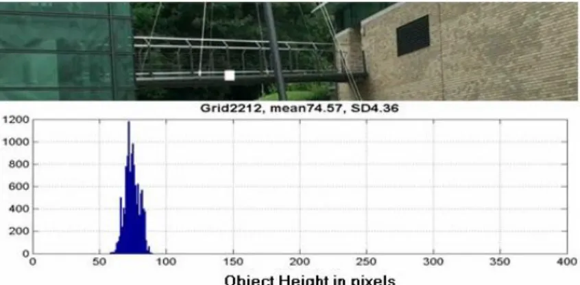
associated with each image patch are modelled with a Gaussian. Note that areas that are not walkable are expected to have few or no observations. Fig. 8 shows the distribution for the image patch marked with a white rectangle in the associated image view.
Fig.8 Pedestrian height distribution for a specific image patch (white rectangle)
4.2 Altitude estimation
Using the reference plane selected as described in section 3.4 and the pedestrian height information for each image patch (Sec. 4.1), the relative altitude of each image patch in the scene with respect to the reference plane is estimated.
Fig. 9 illustrates that for each image patch (red rectangles), an average pedestrian height μHm,n is obtained, as described in section 4.1. Equation 11
computes a position with the same pedestrian height somewhere on the reference plane; yrm,n is called the reference vertical position (green rectangles in Fig. 9).
, , /
r H
m n m n r h
y = R + y (11)
The expansion rate Rr and the horizon yh (where the pedestrian height is
zero) for the reference plane is estimated using the line fitting method described in section 3.2.
Fig.9 Illustration of how altitude is estimated
If there is a difference between the vertical position of the image patch and the reference vertical position yr
m,n, this indicates that the image patch may not be
located on the reference plane but on other planes that are higher or lower than the reference plane. Then, the relative altitude Ar
m,n for the image patch Pm,n is
estimated by taking the difference of vertical positions normalized by the average pedestrian height μH m,n: ( ) , , , / , r r H m n m n m n m n A = y − y (12)
Finally, assuming an average pedestrian height of Hav (e.g. 1.70 meters),
the altitude of each image patch Pm,n can be converted into real units (metres).
r
A visualization of the results of altitude estimation can be seen in Fig. 21 and the evaluation of altitude estimation is shown in Table 3 (results and evaluation section 5.2).
4.3 3D scene model
The relative depth and altitude information are used to build a 3D multi-planar scene model. An automatic method (e.g. as in [8]) is employed to recover the camera’s intrinsic and extrinsic parameters using detected pedestrians on the image plane. Traditional methods of camera calibration (such as Tsai’s calibration) cannot be applied directly, because the scene contains multiple planes. For instance, planes that are high above the ground, will be projected infinitely far away. To address this problem, the reference plane region is used as the dominant ground plane (only objects located on the reference plane are used to recover camera parameters). Then, image pixels in other plane regions are mapped onto the reference plane using Eq. 11 (see Fig. 9b), allowing recovery of all the real world ground positions (in other words, ground plane depth) of image pixels which belong to the other planes (stairs, overpass). Combining the recovered camera parameters with the estimated altitudes, a 3D scene model with real world depth and altitude can be built (please see Fig.22 in section 5.2) for each camera.
5. Dataset and results
5.1 Kingston Hill dataset
We are unaware of any existing public surveillance datasets with scenes containing people moving on multiple planes. Therefore, we have created a new dataset that was captured on the Kingston Hill campus of Kingston University, London and is available1 to researchers who wish to use the results in this paper
as a baseline to be improved upon and future workers to be able to compare their results. We can provide on request data files with annotated ground truth and the results reported here. Because of the extensive human effort required to build a new dataset, the data is understandably limited and we hope that with greater interest from others it will grow in size and variety. Currently, it has views from two cameras monitoring roughly the same area and time synchronized. The videos
were recorded by HD cameras at 25fps with an image resolution of 1280×720. They contain several hours showing a steady flow of a small number of pedestrians walking through the scene. There are three planar structures in the scene including a flat ground area, stairs and an overpass.
Fig.10 Kingston Hill Dataset: a) camera view1, b) camera view 2
5.2 Results and evaluation
Image frames from the HD videos are divided into 10×10 pixel patches. A standard Kalman filter blob tracker with Gaussian background modelling from the OpenCV library [31] (parameters FG_1, BD_CC, CCMSPF, Kalman, RawTracks, HistPVS) is used to obtain the position and size of each pedestrian walking through the scene, resulting in more than two hundred tracks. These are available on request from the authors, as part of the new public dataset, to allow others to reproduce our results.
Walkable regions were extracted using a threshold of Tw experimentally
set to 0.0005 (Sec.3.1) (Fig.11, Fig.12). For both cameras, the common ground area, stairs and an overpass bridge were automatically segmented using data of tracked pedestrians. The plane on the top of the stairs that is visible in the foreground in Fig.12 has not been detected as a walkable region due to pedestrians were avoiding camera 2, which was placed near the top of the stairs.
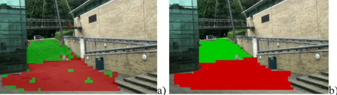
The number of planes in each walkable region is estimated from the number of peaks in the histogram of angles. Fig.13a and Fig.14a indicate the existence of two planes in the first walkable region, while Fig.13b and Fig.14b imply a single plane in the second walkable region. Multiple planes in a single walkable region are segmented by initially merging patches according to Eq.7 (=0.7) (see Fig15a) and then iteratively filtering their labels according to Eq.8 (=0.5) (see Fig. 15b). The segmented planes for all walkable regions are shown in Fig.16.
Fig.11 Walkable regions for cam1
Fig.12 Walkable regions for cam2
Fig.13 Cam1 a) Histogram of angles of lines for walkable region1 b) Histogram of angles of lines for walkable region2
Fig.14 Cam2 a) Histogram of angles of lines for walkable region1, b) Histogram of angles of lines for walkable region2
The correspondence of planes between the two camera FOVs is estimated from the co-occurrence matrix (Sec.3.5), which accumulates the foot positions within each segmented plane (Fig.16) considering all tracked pedestrians in all frames for both cameras. The correct pairs (overpass: A1-A2, stairs: B1-C2, flat area: C1-B2) show the highest co-occurrence scores, according to Table 1.
Fig.15 a) Initial segmentation result for cam1 walkable region1, b) Final segmentation result for cam1 walkable region1.
Fig.16 Scene segmentation results for a) cam1 and b) cam2
Table 1: Co-occurrence matrix for plane correspondence (correct pairs are shown in bold).
Cam1 Cam2
A1 plane B1 plane C1 plane
A2 plane 2340 0 244
B2 plane 466 1433 11359
C2 plane 0 7649 3239
For each correspondence between planes from different camera views, a regional homography mapping is established. We validate the accuracy of mappings by comparing the positions of foot points as seen by one camera and as projected from the other camera. Fig.17 shows examples of pedestrian matching between cameras and projection of trajectories from one camera to the other
mapping errors for different plane regions of different camera views. As pedestrians appear with significantly different heights and widths in different parts of the image, in order to do a fair comparison, all the mapping errors are normalized by the width of the bounding box, and then converted into meters based on an average pedestrian shoulder width of 43cm. As we can see, the overall homography mapping errors are small (7-15cm) except in the stair region of cam2 to cam1 (35cm error). This is caused by occlusion of foot points in the lower section of the stairs in the cam2 view, and as a result objects are inaccurately localized. Compared with methods that assume a single ground plane model, if we took the flat ground area (not considering the stairs and overpass separately) as the “single ground plane”, the homography mapping errors would be infinitely large for the overpass area because it is beyond the horizon line for the “single ground plane”.
Fig.18 shows examples of errors in the homography mapping caused by the occlusion of the lower section of stair in cam2. Since the stair are clearly visible in cam1, objects are located with greater accuracy and reliability in that view. Therefore, when fusing detections from two camera views, greater weight can be given to the camera view which has a smaller homography mapping error, to achieve more accurate localization and tracking of objects.
a) b)
points are the projections of feet from the other camera view using homography b) pedestrian trajectories projected from Cam1 to Cam2 (blue) using region homography.
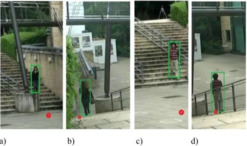
a) b) c) d)
Fig.18 Homography mapping errors caused by the degenerate view of the stairs in cam2 (green boxes are the bounding boxes of pedestrians in the current view, red points are the projections of foot points from the other camera view using homography a) person1 viewed by cam1, b) person1 viewed by cam2, c) person2 viewed by cam1, d) person2 viewed by cam2
Table 2: Average homography mapping error
Flat area Stairs Overpass Cam1 to 2(mean) 0.15m 0.09m 0.12m Cam1 to 2 (STD) 0.09m 0.06m 0.10m Cam 2 to 1(mean) 0.08m 0.35m 0.07m Cam 2 to 1 (STD) 0.05m 0.34m 0.04m
Motion variety in different planes is shown in Fig.19a and Fig.20a (Sec.3.4). The motion vectors associated with the overpass are clearly identified and uniform (mainly in direction 0). Motion vectors on the stairs are fairly uniform (mainly in direction 1). The motion variety of the flat area is clearly greater than the others, and therefore it is selected as the reference plane.
Relative depth maps based on the average pixel-wise pedestrian height are estimated for each image patch for both cameras (Sec.5.1), where different colours represent different pedestrian heights (Fig.19b, Fig.20b).
Fig.19 a) Global motion variety for cam1 with histograms showing motion direction frequency, b) Pedestrian height for each image patch for cam1 (the different colours represent different object heights in pixels)
Fig.20 a) Global motion variety for cam2 with histograms showing motion direction frequency, b) Pedestrian height for each image patch for cam2 (different colours represent different object height in pixels).
Fig.21 a) Estimated altitude for each image patch for cam1, b) estimated altitude for each image patch for cam2, c) side view for camera 1, d) side view for camera 2
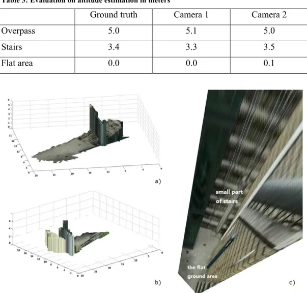
The reference plane and the relative depth map are used to estimate the altitude of each image patch for both camera views (Sec. 4.2). In Fig.21, the (x, y) axes are the image coordinates and the z axis is the estimated altitude. We can see a rough 3D structure of the scene: the flat area, the stairs and the overpass, which is higher than the stairs. In order to evaluate the accuracy of the altitude estimation, we have measured their real heights. The stairs comprise 19 steps: the first 18 steps are 18cm in height, whilst the last step is 16cm. Hence the total height of the stairway is 3.4 meters. The height of the overpass is 5 meters. Table 3 shows the height of the stairs and the overpass estimated for cam1 is 3.3 and 5.1 meters respectively, and 3.5 and 5.0 meters for cam2, giving an overall error of less than 0.1 meter against the true height. Fig. 22 shows the 3D reconstruction of the walkable regions of the scene derived from altitude estimates (Sec.4.3).
Table 3: Evaluation on altitude estimation in meters
Ground truth Camera 1 Camera 2
Overpass 5.0 5.1 5.0
Stairs 3.4 3.3 3.5
Flat area 0.0 0.0 0.1
Fig.22 (a) 3D multiple plane scene model for cam1 (x,y and z axes in meters) (b) 3D multiple plane scene model for cam2 c) projected multi-planes (cam1) caused by using traditional camera calibration method
6. Conclusions and future work
We have considered a typical CCTV installation, with static cameras monitoring a scene containing multiple ground planes, including planar structures such as an overpass and stairs. We have developed a novel method to estimate a multi-planar 3D scene model by exploiting the variation of pedestrian heights across the camera FOV. The method is able to estimate the relative depths of different planes in the scene, segment the image plane into regions that belong to the same geometric plane, identify a reference plane, estimate the relative altitude for each image pixel and finally, build a 3D scene model containing multiple planes. The method has been demonstrated on a scene containing multiple levels and shown to
In addition, in order to extend the method to multiple cameras, the method deals with multiple plane regions in each camera view separately, estimating the homography between different plane regions. The idea of global homography works well when there is a single plane, but effectively what happens outside the plane is ignored. The method proposed in this paper allows the use of multiple homographies corresponding to the multiple planes. These regional homographies allow object correspondence between multiple plane regions from different camera views and furthermore, will facilitate tracking between cameras.
However, there are a few situations that can lead to failure. The method relies on the visibility of the pedestrian’s feet, so if these are occluded (e.g., by a wall or fence) our geometric yardstick of an average person’s measured height will be incorrect. Also, the results of the proposed method may be affected by the accuracy of the tracking. The method will fail if the tracker fails, especially under conditions such as a crowded scene, shadows, occlusions etc. Finally, because homographies are restricted to flat surfaces (or surfaces that may be approximated by planes, e.g., stairs) the method does not cope with surfaces that are not flat, to any significant degree.
In terms of time complexity, learning the model is an off-line process and on a conventional personal computer it takes a matter of hours rather than days. On-line tracking costs depend on the tracker used, which is outside the scope of the paper (for example a Kalman filter would typically be much more time efficient than a particle filter). The only additional computational burden for an online tracking algorithm is associated with computing the homography, which is a negligible cost in matching a pedestrian, as it is based on a simple 3x3 matrix operation.
This research extends the application of ground-plane trackers to multi-planar environments, which are common in the man-made world, and hence opens new directions for tracking objects in more complex environments than have been previously considered, for both single and multiple camera CCTV systems. In this paper we have demonstrated its application using a single scenario, but plan to extend and validate it in a wider range of environments. In particular, we are preparing a follow-on paper that develops multi-camera tracking in a multi-planar environment. The video dataset used has been made available so that other
Acknowledgment
The authors would like to acknowledge BARCO View, Belgium, for their financial support to this project.
References
1. M.D. Breitenstein, E. Sommerlade, B. Leibe, L. van Gool and Ian Reid,:“Probabilistic Parameter Selection for Learning Scene Structure from Video”, British Machine Vision Conference (BMVC'08), September (2008)
2. D.Greenhill, J.R.Renno, J.Orwell, G.A.Jones, “Occlusion Analysis: Learning and Utilising Depth Maps in Object Tracking, in Image and Vision Computing”, Special Issue on the 15th Annual British Machine Vision Conference 26(3), pp. 430-44, Elsevier Publishing, March (2008)
3. J.R.Renno, J.Orwell, G.A.Jones, “Learning Surveillance Tracking Models for the Self-Calibrated Ground Plane”, British Machine Vision Conference, September, Cardiff, pp. 607-616. (2002)
4. N. Krahnstoever and P.Mendonca, “Autocalibration from Tracks of Walking People”, British Machine Vision Conference, Edinburgh, UK (2006)
5. C. Huang, Bo Wu, and R. Nevatia, “Robust Object Tracking by Hierarchical Association of Detection Responses”, ECCV, Marseille, France, pp.788-801. (2008)
6. D.Hoiem, A. A.Efros, and M.Hebert, “Putting objects in perspective, International Journal of Computer Vision”, pp. 0920-5691 (2008).
7. A.Saxena, M.Sun, and A.Ng: “Make3D: Learning 3D Scene Structure from a Single Still Image”, IEEE Trans on Pattern Analysis and Machine Intelligence, pp. 824-840 (2009) 8. F.Lv, T.Zhao, and R.Nevatia, “Camera calibration from video of a walking human, IEEE
Trans on Pattern Analysis and Machine Intelligence”, pp.1513-1518 (2006)
9. L.Lin, L.Zhu, F.Yang, T.Jiang, “A novel pixon-representation for image segmentation based on Markov random field”, Image and Vision Computing, Vol. 26, No. 11. pp. 1507-1514, November (2008)
10. C. C.Loy, T.Xiang, S.G.Gong, “Modelling Multi-object Activity by Gaussian Processes”, British Machine Vision Conference (BMVC’09) (2009)
11. C.Madden, E. D.Cheng, M.Piccard, “Tracking people across disjoint camera views by an illumination-tolerant appearance representation”, Machine Vision Applications, pp. 18(3-4): 233-247 (2007)
12. L.A.F.Fernandes. M.M.Oliveira, “Real-time line detection through an improved hough transform voting scheme”, Pattern Recognition, Vol. 41, No. 9, pp.299-314, September
13. M.Xu, T.J.Ellis, “Partial observation vs. blind tracking through occlusion, British Machine Vision Conference”, BMVA, September, Cardiff, pp. 777-786 (2002)
14. W.S.Cleveland, S.J.Devlin, “Locally-Weighted Regression: An Approach to Regression Analysis by Local Fitting”. Journal of the American Statistical Association 83 (403): 596-610 (1988)
15. D.Rother, K.A.Patwardhan, G.Sapiro, “What Can Casual Walkers Tell Us About A 3D Scene? ”, ICCV2007, pp.1-8, IEEE 11th International Conference on Computer Vision (2007)
16. J.Black, T. Ellis. “Multi camera image tracking”, In Proc. IEEE Workshop on Performance Evaluation of Tracking and Surveillance. (2001)
17. C. Stauffer and K. Tieu., “Automated multi-camera planar tracking correspondence modelling”, In proceedings of CVPR, pp.259. (2003)
18. S. Khan, and M.Shah, “Consistent Labeling of Tracked Objects in Multiple Cameras with Overlapping Fields of View”, IEEE Trans. on Pattern Analysis and Machine Intelligence, Vol. 25, No. 10, pp.1355-1360 (2003)
19. M. Borg, D. J.Thirde, J.M. Ferryman, F. Fusier, V. Valentin, F. Brémond, M. Thonnat, J. Aguilera, M. Kampel, “Automated Scene Understanding for Airport Aprons”, The 18th Australian Joint Conference on Artificial Intelligence (AI05) in Sydney, Australia, December, Vol. 3809, pp. 593-603 (2005)
20. J. Black, T. Ellis, D. Makris, “Wide Area Surveillance With a Multi Camera Network”, In: Intelligent Distributed Surveillance Systems, London, pp. 21-25 (2004)
21. O. Chum and J. Matas. “Randomized ransac with T(d,d) test”, In Proceedings of the British Machine Vision Conference, volume 2, pages 448-457 (2002)
22. M. Wilczkowiak, E. Boyer, and P. Sturm, “Camera Calibration and 3D Reconstruction from Single Images Using Parallelepipeds,” Proc. Int’l Conf. Computer Vision, pp. 142-148 (2001)
23. F. Yin, D. Makris, S.A. Velastin, J. Orwell, “Quantitative Evaluation of Different Aspects of Motion Trackers under Various Challenges,” in 'Annals of the British Machine Vision Association', (5) British Machine Vision Association, pp. 1-11. (2010)
24. J. Black, T. Ellis, “Multi camera image tracking,” in 'Image and Vision Computing', 24(11) Elsevier, Nov 1, pp. 1256-1267. ISBN/ISSN 0262-8856. (2006)
25. D. Fouhey, V. Delaitre, A. Gupta, A. A. Efros, I. Laptev, J. Sivic. “People watching: Human actions as a cue for single view geometry”, Computer Vision–ECCV 2012. Springer Berlin Heidelberg, pp.732-745.(2012)
26. F. Yin, D. Makris, J. Orwell, S.A. Velastin. “Learning Non-coplanar Scene Models by Exploring the Height Variation of Tracked Objects”, ACCV 2010, Lecture Notes in Computer Science, 2011, Volume 6494, pp 262-275
27. R. Hartley and A. Zisserman. Multiple View Geometry in Computer Vision. Cambridge University, Press, Cambridge, UK, 2000.
29. D. G. Lowe, "Distinctive image features from scale-invariant keypoints." International journal of computer vision 60.2 (2004): 91-110.
30. N. Noceti, L. Balduzzi, F. Odone. "What Epipolar Geometry Can Do for Video-Surveillance." In Image Analysis and Processing–ICIAP 2013, pp. 442-451. Springer Berlin Heidelberg, 2013
31. OpenCV (n.d.). Open source computer vision library. http://www.opencv.org/ (accessed: December 2013).