RADAR Signal Processing Using Multi-Objective Optimization Techniques

(1)

RADAR Signal Processing using

Multi-Objective Optimization Techniques

Vinod Kumar

Roll no. 213EC6256

Department of Electronics and Communication Engineering National Institute of Technology, Rourkela

Rourkela, Odisha, India 2015

(2)

RADAR Signal Processing using

Multi-Objective Optimization Techniques

Thesis submitted in partial fulfillment of the requirements for the degree of

Master of Technology

in

Signal & Image Processing

by

Vinod Kumar

Roll no. 213EC6256

under the guidance of

Prof. Ajit Kumar Sahoo

Department of Electronics and Communication Engineering National Institute of Technology, Rourkela

Rourkela, Odisha, India 2015

(3)

(4)

National Institute of Technology

Rourkela

CERTIFICATE

This is to certify that the work in the thesis entitled ”RADAR Signal Processing using Multi-Objective Optimization Techniques”submitted byVinod Kumaris a record of an original work carried out by him under my supervision and guidance in partial fulfillment of the requirements for the award of the degree ofMaster of TechnologyinSignal & Image Processingfrom National Institute of Technology, Rourkela. Neither this thesis nor any part of it, to the best of my knowledge, has been submitted for any degree or academic award elsewhere.

Prof. Ajit Kumar Sahoo

Assistant Professor Department of ECE National Institute of Technology Rourkela

(5)

National Institute of Technology

Rourkela

DECLARATION

I certify that

1. The work contained in the thesis is done by myself under the supervision of my supervisor.

2. The work has not been submitted to any other Institute for any degree or diploma.

3. Whenever I have used materials (data, theoretical analysis, and text) from other sources, I have given due credit to them by citing them in the text of the thesis and giving their details in the references.

4. Whenever I have quoted written materials from other sources, I have put them under quotation marks and given due credit to the sources by citing them and giving required details in the references.

(6)

Acknowledgment

This work is one of the most important achievements of my career. Completion of my project would not have been possible without the help of many people, who have constantly helped me with their full support for which I am highly thankful to them.

First of all, I would like to express my gratitude to my supervisor Prof. Ajit Kumar Sahoo, who has been the guiding force behind this work. I want to thank him for giving me the opportunity to work under him. He is not only a good Professor with deep vision but also a very kind person. I consider it my good fortune to have got an opportunity to work with such a wonderful person.

I am obliged to Prof. K.K. Mahapatra, HOD, Department of Electronics and Communication Engineering for creating an environment of study and research. I am also thankful to Prof. A.K. Swain, Prof. L.P. Roy, Prof. S. Meher, Prof. S. Maiti, Prof. D.P. Acharya and Prof. S. Ari for helping me how to learn. They have been great sources of inspiration.

I would like to thank all faculty members and staff of the ECE Department for their sympathetic cooperation. I would also like to make a special mention of the selfless support and guidance I received from PhD Scholar Mr. Sanand Kumar and Mr. Nihar Ranjan Panda during my project work.

When I look back at my accomplishments in life, I can see a clear trace of my family’s concerns and devotion everywhere. My dearest mother, whom I owe everything I have achieved and whatever I have become; my beloved late father, who always believed in me and inspired me to dream big even at the toughest moments of my life; and sisters; who were always my silent support during all the hardships of this endeavor and beyond.

(7)

Abstract

Pulse compression technique is used in radar system to achieve the range res-olution of short duration pulses and Signal to Noise Ratio (SNR) of long duration pulses. In pulse compression technique a long duration pulse is transmitted with either a frequency or phase modulation. At receiver end, we use matched filter, which accumulate the energy of long pulse into a short pulse. Linear Frequency Modulated (LFM) pulse is one type of signal used in radar. The matched filter response of LFM pulse gives side lobe of about −13dB, which can be improved by using windowing, adaptive filtering and optimization techniques. In wide-band radar, for good range resolution, very wide bandwidth is used. The conventional hardware may not be able to sustain this large bandwidth. So the wide-band signal is split into narrow-band signals. These narrow-band signals are transmitted and recombined coherently at receiver’s end.

In narrow-band signals, frequency changes linearly for complete duration of pulse. We change the center frequency of each LFM pulse by introducing a fre-quency step between consecutive pulses. Resultant signal is known as Stepped Frequency Pulse Train (SFPT) or Synthetic Wide-band Waveform (SWW). The disadvantage of SFPT is that when the product of pulse duration and frequency step become more than one, the Autocorrelation Function (ACF) of SFPT yields undesirable peaks, known as grating lobes. Along with grating lobe, the higher peak side lobe either can hides the small targets or can cause the false alarm detec-tion. Also the wide main lobe width deteriorate the range resolution capability of the signal. Many analytic techniques have been proposed in the literature to select the SFPT parameter to suppress the grating lobe, without paying much attention to side lobe and main lobe width. Multi-Objective Optimization (MOO) methods are also used for this purpose.

In this work we compare three MOO algorithms to find the optimized param-eter of SFPT. The optimization problem is studied in two ways: In first we take

(8)

objective of minimization of grating lobes and peak side lobe level. The constraint is of increase in bandwidth. In second problem, our aim is to minimize the main lobe width, which improves the resolution. The objective functions for second problem are minimization of main lobe width and peak side lobe level. We don’t want high grating lobe amplitude, so we add a constraint, which restrict the maxi-mum grating lobe amplitude below a threshold value. Simulations are carried out for different range of parameter values and the simulation result shows the poten-tial of the MOO approach.

Keywords: ACF, Grating Lobes, Matched filter, Multi-objective optimization, Pulse Compression, Side lobes.

(9)

List of Figures

2.1 Pulsed RADAR waveform . . . 8

2.2 Transmitter and receiver ultimate signals . . . 9

2.3 Block diagram of a pulse compression radar system . . . 10

2.4 Block diagram of a matched filter . . . 11

2.5 Phase modulated waveform . . . 18

2.6 The instantaneous frequency of the LFM waveform over time . . . 19

2.7 Real Part of LFM signal. B=200MHz,t =10µsec. . . 20

2.8 Imaginary Part of LFM signal. B=200MHz,t =10µsec. . . 21

2.9 Spectrum of LFM signal. B=200MHz,t =10µsec. . . 21

2.10 Ambiguity function plot of single pulse, constant frequency signal 22 2.11 Ambiguity function plot of single pulse, constant frequency signal for zero Doppler cut. . . 22

2.12 Ambiguity function plot of single pulse, constant frequency signal for zero delay cut. . . 23

2.13 Ambiguity function plot of single LFM pulse . . . 23

2.14 Ambiguity function plot of single LFM pulse zero Doppler cut . . 24

2.15 Ambiguity function plot for LFM pulse train. Number of pulse N =3 . . . 24

2.16 Ambiguity function plot for LFM pulse train for zero Doppler cut. Number of pulseN =3 . . . 25

(13)

List of Figures

3.2 SFPT for Tp∆f =3, TpB=4.5 andN =8. Top shows |R1(τ)| in

solid line and|R₂(τ)| in dashed line. Bottom shows ACF in dB. . 31

3.3 Constant frequency pulse train for Tp∆f =3, TpB=0 and N =8. Top shows|R₁(τ)|in solid line and|R2(τ)|in dashed line. Bottom shows ACF in dB. . . 31

4.1 Crowding distance calculation . . . 42

4.2 NSGA-II procedure . . . 44

4.3 Possible cases for the archive controller . . . 52

4.4 Insertion of a new solution (lies inside the boundary) in Adaptive grid. . . 53

4.5 Insertion of a new solution (lies outside the boundary) in Adaptive grid. . . 53

4.6 Behavior of mutation operator . . . 55

4.7 The performance metric Hypervolume (HV) in MOO. . . 56

4.8 Number of generation vs objective function value for G-1 problem 59 4.9 Number of generation vs objective function value for G-6 problem 59 4.10 Pareto front obtained for CTP-2 problem . . . 60

5.1 Pareto front obtained forTp∆f = [2,10]and c= [2,10] . . . 64

5.2 Pareto front obtained forTp∆f = [2,10]and c= [2,5] . . . 64

5.3 ACF plot of SFPT for F₁ = 0. Parameter of SFPT are obtained from NSGA-II algorithm. Tp∆f = 2, c =5 and tpB =12. Top shows |R₁(τ)| by solid line and |R₂(τ)| by dashed line. Bottom shows ACF in dB . . . 67

5.4 ACF plot of SFPT for F₁ = 0. Parameter of SFPT are obtained from MOPSO Algorithm. Tp∆f =3, c =5 and TpB = 18. Top shows |R₁(τ)| by solid line and |R2(τ)| by dashed line. Bottom shows ACF in dB . . . 67

(14)

List of Figures

5.5 ACF plot of SFPT forF₁ =0.01. Parameter of SFPT are obtained from NSGA-II Algorithm. Tp∆f =2, c=5.12 andTpB=12.24.

Top shows |R₁(τ)| by solid line and |R₂(τ)| by dashed line.

Bot-tom shows ACF in dB . . . 68 5.6 ACF plot of SFPT for F₁ = 0.01. Parameter of SFPT are

ob-tained from MOPSO Algorithm. Tp∆f =2.93,c=5.06 andTpB=

17.75. Top shows|R₁(τ)|by solid line and|R₂(τ)|by dashed line.

Bottom shows ACF in dB . . . 68 5.7 Pareto front obtained forTp∆f = [2,10]and c= [2,10] . . . 69

(15)

List of Tables

3.1 Weighting function to reduce the side lobes . . . 33

4.1 Calculation of constraint violation measure . . . 48

5.1 Performance metrics Obtain using MOO Algorithms for

Problem-1 . . . 66

(16)

List of Algorithms

1 Nondominated Sorting Genetic Algorithm-II . . . 41 2 Infeasibility Driven Evolutionary Algorithm . . . 46 3 Multi Objective Particle Swarm Optimization Algorithm . . . 51

(17)

List of Acronyms

Acronym

Description

ACF

Autocorrelation Function

AF

Ambiguity Function

AWGN

Additive White Gaussian Noise

BW

Bandwidth

IDEA

Infeasibility Driven Evolutionary Algorithm

CW

Continuous Wave

LFM

Linear Frequency Modulation

NSGA

Nondominated Sorting Genetic Algorithm

MOO

Multi-Objective Optimization

MOPSO

Multi-Objective Particle Swarm Optimization

PCR

Pulse Compression Ratio

PSD

Power Spectral Density

PSO

Particle Swarm Optimization

PSR

Peak to Side lobe Ratio

RADAR

Radio Detection and Ranging

SFPT

Stepped Frequency Pulse Train

SNR

Signal to Noise Ratio

(18)

Chapter 1 Thesis Overview

Background Motivation Objective Thesis Organization

(19)

Chapter 1 Thesis Overview

1.1 Background

From last few decades, radar system is widely used in many applications like military and commercial. The reason for the widespread use of radar is advance-ment in the signal generation and processing technology. In military applications, high range resolution radar systems are always a top priority. High range resolu-tion radar design is hindered by the high bandwidth requirement.

Applying modulation is one way to increase the bandwidth of the signal. Linear frequency modulated (LFM) pulse is one such signal that gives us good range resolution. Range resolution can be further improved by using Stepped Frequency Pulse Train (SFPT). The SFPT employ inter-pulse, pulse compression technique. In this technique, a frequency step, ∆f, is applied to consecutive pulses. Because

of frequency step, carrier frequency changes linearly. Applying frequency step∆f,

on the successive pulse, increase the signal bandwidth. The bandwidth of SFPT become equal to the product of number of coherently integrated pulse, N, and a frequency step size, ∆f. SFPT overall become a wide-band signal, but each pulse

is a narrow-band signal. This feature makes the design of receiver simpler.

The key advantage of the SFPT as compared to other radar signal is its high range resolution with wide overall bandwidth and small instantaneous bandwidth. Implementation of SFPT is simple. The disadvantage of SFPT is that it exhibits high side lobe at location τg =g/∆f. These side lobes, known as grating lobes,

have comparable energy as to main lobe. Grating lobe in some applications can hide the weak target or can cause a false alarm, so they are not desirable in the

(20)

Chapter 1. Thesis Overview

output. Also when we improve the range resolution of a pulse, its main lobe width decreases. From the properties of ambiguity function, if we try to squeeze the main lobe, the volume removed from the main lobe must appear somewhere else. This volume appears in the form of side lobes. So the better the range resolution, the more side lobes it shows. These side lobes are also not desirable. Proper selection of the parameter of SFPT can yield an optimum range resolution with suppressed or no grating low and minimized peak side lobe.

1.2 Motivation

Many efforts have been made, in the available literature, to suppress the side lobes in the matched filter output of the radar system. Different mismatch filters are proposed in past to improve the peak to side lobe ratio, but the mismatched filters provide weak convergence performance. So there is a need to improve the mismatch filters.

In polyphase and LFM waveforms, amplitude weighing techniques can be used to suppress side lobes. When there is Doppler shift in the waveform, the matched filter gives us degraded PSR. Under such situations, it is required to improve the PSR.

The matched filter output for stepped frequency LFM pulse train is its auto-correlation function. Stepped frequency pulse train shows the grating lobe in the matched filter output. Grating lobe appears because of a constant frequency step. Many techniques are available in the literature to suppress the grating lobe, but they ignore the PSR and main lobe width. Therefore, there is a need to develop methods by which we can choose the parameters of stepped frequency waveform such that it provides high range resolution, lower grating lobes and reduced side lobes.

1.3 Objective

The objective of this work is to find out the optimum parameter of stepped frequency pulse train, which can yield good range resolution with suppressed or

(21)

eliminated grating lobe. With grating lobe suppression, we also aims for the min-imization of the peak side lobe. In the radar system, if we try to suppress or eliminate the grating lobe, then the peak side lobe might increase (From ambigu-ity function property). For us, both side lobes and grating lobe are undesired. We want to eliminate both grating lobe and side lobe.

Here we have a conflicting situation, minimizing grating lobe result in in-creased side lobe. To deal with this situation we use Multi-Objective Optimiza-tion (MOO) techniques. MOO techniques used to simultaneously optimized one or more than one objective function. In this work, we use NSGA-II, MOPSO and IDEA algorithms to find the optimized parameter of stepped frequency pulse train which can give us good range resolution, minimum grating lobe amplitude, and low peak side lobe.

1.4 Thesis Organization

1. Chapter 1: Thesis Overview 2. Chapter 2: Introduction

This chapter introduces the basics concept of pulse compression, matched filter, ambiguity functions and various signals used in radar. MATLAB simulation of some signals with their ambiguity function is also presented in this chapter.

3. Chapter 3: Coherent Train of LFM Pulses

In this chapter, we discussed about the Coherent Train of LFM Pulses (stepped frequency pulse train). We, first derived the expression for ACF of SFPT, then grating lobe and side lobes are explained. Literature review for side lobe and grating lobe is presented next. Problem used for optimization is formulated in the next section and finally the conclusion for the chapter is presented.

4. Chapter 4: Multi-Objective Optimization

Multi-objective optimization techniques are discussed in this section. The ba-sic concept is presented first. Then we discuss the MOO techniques used to find the optimized parameter of SFPT. In MOO techniques, first we discuss

(22)

the Nondominated Sorting Genetic algorithm (NSGA-II), then Multi-Objective Particle Swarm Optimization (MOPSO) and at last Infeasibility Driven Evolu-tionary Algorithm (IDEA) is discussed. Simulation of some standard test prob-lem is done for all three optimization algorithms. In last section conclusion for the chapter is presented.

5. Chapter 5: Simulation Results

This chapter presents the simulation results for the problem formulated in chap-ter 3. MATLAB simulation using MOO algorithms for both problems are shown for various values of signal parameters. Results obtain using MOO al-gorithms is also compared on the basis of a performance comparison metrics.

6. Chapter 6: Conclusion and Future Work

In this chapter the conclusion of this work is presented. This chapter also gives details about the further research work which can be attempted subsequently.

(23)

Chapter 2 Introduction

Introduction Pulse Compression Matched Filter Ambiguity Function Radar Signals Simulation Results Conclusion

(24)

Chapter 2 Introduction

2.1 Introduction

RADAR is an acronym of RAdio Detection And Ranging. Radar is used in many applications to find the presence of an object within the search space. Apart from just giving the existence of the object, modern radars are capable of providing many other information about the properties of the object like range, altitude, size, direction, speed, etc. The radar antenna transmits an electromagnetic signal into the search space. The transmitted signal is reflected by the object present (if any). Radar antenna receives the reflected signal, known as echo, from the object. The echoes are processed to extract the information about the object. There are two type of radar, Continuous Wave (CW) radar and pulsed radar. The CW radar continuously transmits the signal. CW radar has the advantage of unambiguous Doppler measurement, but it require two antennas. Also due to the continuous nature of the signal the target range measurement of CW radar is ambiguous.

In the modern era, we use pulse radar system because it provides accurate range information. Also, the hardware requirement is less since transmitter and receiver can share the same antenna. The unambiguous range of pulsed radar is given by [1, p. 3]

Ru =

cTr

2 F (2.1)

Where c is the speed of light, Tr is the pulse repetition time. One such pulse

(25)

ex-Chapter 2. Introduction

Figure 2.1: Pulsed RADAR waveform

pressed as [2, p. 5], [3]

∆R= cTp

2 = c

2B (2.2)

HereB is for the bandwidth of the pulse. Pulse width decides the range resolu-tion of the signal. Low pulse width gives the better range resoluresolu-tion, but low pulse width decrease the average pulse energy (Pavg = Pt_TTP

r ) [1, p. 74]. So we have to

transmit more power to have reasonable average pulse energy.

The minimum detectable signal to noise ratio is given by [1, p. 34] as

S N min = PtGAeσ (4π)2kT₀BFnR4max (2.3)

To detect signal, Signal to Noise Ratio (SNR) should be more than _NS_min. For constant radar parameter _NS_min is high for high Pt. So we can’t detect signals

with low SNR when we transmit high power. This is one drawback of using low pulse width.

In Radar system, we have a conflicting problem. We want pulse width to low for good range resolution, but with low pulse width, we have to transmit more power to detect weak signals. To transmit low power(detect low SNR signal) with good range resolution, pulse compression techniques is employed in radar systems.

2.2 Pulse Compression

Equation 2.2 gives the range resolution for a radar signal. The time duration of the unmodulated pulse is inversely proportional to its bandwidth. Low time duration and high bandwidth signal exhibits an excellent range resolution, but we can not increase the bandwidth of the signal (or decrease the time duration )

(26)

Chapter 2. Introduction

Figure 2.2: Transmitter and receiver ultimate signals

indefinitely. Fourier theory says that, for the signal having bandwidth B, the time period can not become less than 1/B. In other words, the product of time and bandwidth can not become less than unity. For large distance communication, short duration pulses require high energy. The equipment used in high power radar are bulky, requires more space and they increase the total cost of the system. Therefore, high power transmission is restricted by the transmitter.

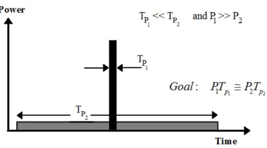
The maximum detection range depends upon the energy of the received echo signal. For echo signal to have high energy, transmitted pulse should have high energy. The energy of received echo depends on the pulse duration and peak transmitted power. We can achieve the average power of low pulse width and high peak transmission power by transmitting low peak power with high pulse width. Figure 2.2 shows two such pulse; both are having different pulse width, but their energy is same.

Frequency or phase modulation technique can be used to enhance the band-width of a large duration pulse. Increase in bandband-width also improves the range resolution. In pulse compression technique, we transmit low peak power, long duration pulse. This pulse is either phase or frequency modulated. At the re-ceiver side, we pass this received signal through matched filter. Matched filter accumulate the energy of long pulse into a short pulse. The performance of pulse

(27)

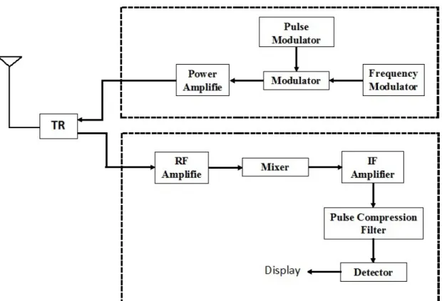
Figure 2.3: Block diagram of a pulse compression radar system

compression is measured by Pulse Compression Ratio (PCR), and it is defined in [1] as

PCR= pulse,width be f ore compression

pulse width a f ter compression (2.4) The higher the value of PCR, the better will be the compression.

Figure 2.3 shows the block diagram of a radar pulse compression system. The transmitted signal is either frequency or phase modulated to enhance the band-width. Transceiver (TR) is a switching unit, which helps to use the same antenna as a transmitter and as a receiver. Matched filter is used in pulse compression system at the receiver side. Its frequency spectrum matches with that of transmit-ted signal. The matched filter gives correlation between two signals (transmittransmit-ted and received pulses). When we give received pulse as an input to matched filter, then we will get maximum SNR, compressed pulse as an output, if properties of received pulse matches to the transmitted pulse.

(28)

Figure 2.4: Block diagram of a matched filter

2.3 Matched Filter

A radar detects the presence of an object by echo signal reflected from the ob-ject. Additive White Gaussian Noise (AWGN) present in search space may cor-rupts the reflected signal. The noise power in received signal may be comparable with original signal power, which gives us the low value of SNR. The maximum probability of detection depends on the SNR [1, p. 43]. So to maximize SNR, matched filter is employed. The matched filter impulse response is expressed in terms of the signal for which the filter is matched. When the exactly matched sig-nal (plus white noise) is passed to matched filter, it gives maximum SNR [4, p. 20]. The maximum SNR occurs at a particular instant of time. This time is a design parameter.

The block diagram of matched filter is shown in Figure 2.4. An input signal s(t) passes through the channel, which corrupts the signal by adding AWG noise. Let the two-sided Power Spectral Density (PSD) of the AWGN channel is N0

2 . We want to find the filter transfer function H(f) which results in maximum SNR at a predetermined time delay t₀. The output SNR of matched filter shown in Figure 2.4 is given by [4, p. 24] S N out = |s0(t0)| 2 n2₀(t) (2.5)

(29)

at the time instant where we want to maximize the SNR. The mean square value of noise is presented asn2₀(t) . Let the Fourier transform ofs(t) is S(f). s₀(t) can be obtained as s₀(t) = ∞ Z −∞ H(f)S(f)ej2πf t_{d f} _(2.6)

The value of s₀(t) att =t₀ is given by s₀(t₀) =

∞ Z

−∞

H(f)S(f)ej2πf t0_{d f} _(2.7)

The mean square value of noise

n2₀(t) = N0 2 ∞ Z −∞ |H(f)|2d f (2.8) Substituting equation 2.7 and 2.8 into 2.5 gives

S N out = ∞ R −∞ H(f)S(f)ej2πf t0_{d f} 2 N0 2 ∞ R −∞ |H(f)|2d f (2.9)

Using Schwarz inequality the numerator of 2.9 can be written as

∞ Z −∞ H(f)S(f)ej2πf t0_{d f} 2 ≤ ∞ Z −∞ |H(f)|2d f ∞ Z −∞ S(f)ej2πf t0_{d f} _(2.10) Equality in equation 2.10 if H(f) =K₁ h S(f)ej2πf t0 i∗ =K₁S∗(f)e−j2πf t0 _(2.11)

Where K1 is any arbitrary chosen constant and ∗ is for complex conjugate. Using the relationship of S(f) and H(f) into equation 2.5, which corresponds to maxi-mum SNR S N out = ∞ R −∞ |S(f)|2d f N₀ 2 = 2E N₀ (2.12) 12

(30)

The energy of finite time signal s₀(t) is given by E = ∞ Z −∞ |s(t)|2dt = ∞ Z −∞ |S(f)|2d f (2.13) From equation 2.13, it is clear that the maximum SNR depends on the energy of the signal, not on the shape of the signal. Applying inverse Fourier transform on equation 2.11 gives the matched filter impulse response as

h(t) =K₁s∗(t₀−t) (2.14) This equation says that the impulse response of matched filter is a delayed version of input signal with complex conjugate.

The output at time t =t₀ is s₀(t₀) =K₁ ∞ R −∞ S(f)S∗(f)e−j2πf t0_ej2πf t0_{d f} =K₁ ∞ R −∞ |S(f)|2d f =K1E (2.15)

This equation say that at predefined delayt =t0 output is the energy of the signal (assume K₁ =1), regardless of the type of waveform. The output of the matched filter is expressed as s0(t) =s(t)⊗h(t) = ∞ R −∞ s(τ)h(t−τ)dτ = ∞ R −∞ s(τ)K₁s∗(τ−t+t0)dτ = ∞ Z −∞ s(τ)s∗(τ −t)dτ K1=1,t0=0 (2.16)

Where ⊗is for linear convolution. The right hand side of equation 2.16 is known as autocorrelation function (ACF) of the input signals(t).

(31)

2.3.1 Matched filter for a narrow bandpass signal

Modern radar generally uses narrow-band signals. The Fourier transform of the baseband signal is centered at a carrier frequency ωc and covers a frequency band

of 2B. The fundamental representation of baseband signal is [4, p. 20]

s(t) =g(t)cos[ωct+φ(t)] (2.17)

where g(t) and φ(t) are the natural envelop and instantaneous phase of the s(t) respectively. Another representation of base band signal is

s(t) =gc(t)cosωct−gs(t)sinωct (2.18)

where gc(t) is in-phase component and gs(t) is quadrature component, expressed

as

gc(t) =g(t)cosφ(t)

gs(t) =g(t)sinφ(t)

(2.19)

gc(t) and gs(t) both are bounded by a range of frequency, denoted as W both

signals can be viewed as baseband signals. The complex envelop of s(t)is given by

u(t) =gc(t) + jgs(t) (2.20)

The complex envelop gives another expression to represent the signal

s(t) =Re{u(t)exp(jωct)} (2.21)

The natural envelop of signal is equal to the magnitude of complex envelop

s(t) =|u(t)| (2.22)

Putting the value of|u(t)|gives another expression to represent narrow band signal as s(t) = 1 2u(t)exp(jωct) + 1 2u ∗_(t)_exp(₋ jωct) (2.23)

Using Equation 2.23 in Equation 2.16 yields [4, p. 29] s₀(t) = K1 4 ∞ R −∞ u(τ)ej2πf0τ₊_u∗_(τ_)e−j2πf0τ n u∗(τ−t+t0)e−j2πf0(τ−t+t0)+u(τ−t+t0)ej2πf0(τ−t+t0) o dτ (2.24) 14

(32)

on performing the cross product, give us s0(t) = K₄1exp[jωc(t−t0)] ∞ R −∞ u(τ)u∗(τ−t+t0)dτ +K1 4 exp[−jωc(t−t0)] ∞ R −∞ u∗(τ)u(τ−t+t₀)dτ +K1 4 exp[jωc(t−t0)] ∞ R −∞ u∗(τ)u∗(τ−t+t₀)exp(−j2ωcτ)dτ +K1 4 exp[−jωc(t−t0)] ∞ R −∞

u(τ)u(τ−t+t₀)exp(j2ωcτ)dτ

(2.25)

the second and fourth part of the above equation is complex conjugate of first and third part respectively. So it can be written as

s₀(t) = K1 2 Re exp[jωc(t−t0)] ∞ R −∞ u(τ)u∗(τ−t+t₀)dτ +K1 2 Re exp[jωc(t−t0)] ∞ R −∞ u∗(τ)u∗(τ−t+t0)exp(−j2ωcτ)dτ (2.26) second part of Equation 2.26 is Fourier transform of

∞ R

−∞

u∗(τ)u∗(τ−t+t₀) eval-uated at ω =ωc. Since s(t) is a narrow band signal and its spectrum is centered

around ωc. So spectrum of its complex envelop signal u(t) is cut well below ωc,

and we can neglect the second term.

s₀(t)≈ K1 2 Re exp[jωc(t−t0)] ∞ R −∞ u(τ)u∗(τ−t+t₀)dτ Re K1 2 exp(−jωct0) ∞ R −∞ u(τ)u∗(τ −t+t₀)dτ exp(jωct) (2.27)

Let we define a new complex envelop:

u0(t) =Ku ∞ Z −∞ u(τ)u∗(τ−t+t0)dτ, Ku= K₁ 2 exp(−jωct0) (2.28) Matched filter output can be written as

s₀(t)≈Re{u₀(t)exp(jωct)} (2.29)

Above two equations shows that the output is matched to narrow-band pulse. Pass-ing the complex envelope of u(t) through the matched filter gives the complex

(33)

envelop of outputu₀(t).

2.4 Ambiguity Function

Ambiguity function (AF) is the output of matched filter when the input to matched filter is received signal with a Doppler shiftν and a time delayτ relative to a nominal value expected by the filter. The AF can be expressed as [4, p. 34]

|χ(τ,ν)|= ∞ Z −∞ u(t)u∗(t+τ)ej2π νtdt (2.30)

Here u(t) represent the complex envelope of the signal. A positive value of τ means target is moving away from the radar reference position. A positive value ofν implies that is moving towards the radar.

2.4.1 Properties of Ambiguity Function 1. Property 1: Maximum at(0,0)

|χ(τ,ν)| ≤ |χ(0,0)|= (2E)2 (2.31) This property says that the AF has a maximum value at the origin, which is the actual location of the target, when the Doppler shiftν =0. The maximum value is(2E)2, where E is the energy of echo signal.

2. Property 2: Constant volume

∞ Z −∞ ∞ Z −∞ |χ(τ,ν)|2dτdν = (2E)2 (2.32)

The total volume under AF is constant and equal to (2E)2.

From property 1 and 2, we can say that, if we try to squeeze the AF to a nar-row peak at origin, then the peak can not exceed the value of(2E)2. Further, the volume removed from the peak must emerge somewhere else [4, p. 35].

3. Property 3: Symmetry with respect to the origin

|χ(−τ,−ν)|=|χ(τ,ν)| (2.33)

(34)

This property says that we only need to study two adjacent quadrants to get complete information about AF.

4. Property 4: LFM effect

Let a complex envelopu(t) has an AF

u(t)⇔ |χ(τ,ν)| (2.34) then adding LFM, the AF of resultant signal is given as:

u(t)ejπkt2 _{⇔ |}

χ(τ,ν−kτ)| (2.35) This property says that adding LFM effect, shears the resulting AF.

2.5 Radar Signals

To get the effect of bandwidth of the low pulse width signal in the high pulse width signal, we apply some kind to modulation to the input signal. Normally phase or frequency modulated signals are used in radar. These two modulated signals are described below.

2.5.1 Phase Modulated Signal

The increase in bandwidth can be achieved by using phase modulation tech-niques. In phase modulation, we have a pulse of durationTp. This pulse is divided

into N sub-pulses, each of having duration tb as shown in Figure 2.5. Each sub

pulse is assigned with a phase value ϕi, where i =1,2,3, ...N. The phase ϕi of

sub pulse is selected in accordance with a coding sequence. The basic phase-code modulation technique is binary coding. It requires two phases. The binary code is a sequence of either 0 and 1 or+1 and −1. The transmitted signal phase changes between and with respect to the sequence of elements. Since the frequency of transmission is not always a multiple of the reciprocal of the sub pulse interval, hence at the phase reversal points the phase coded signal is usually discontinuous. The PCR of phase coded pulse is obtained as

PCR= Tp

(35)

Figure 2.5: Phase modulated waveform

The compression ratio is equivalent to the number of elements in the code, i.e., the number of sub-pulses in the waveform. Matched filter is used at the receiver end to obtain the compressed pulse. The compressed pulse width at the half-amplitude point is usually equal to the width of the sub pulse. Hence, the range resolution is directly proportional to the time duration of one sub pulse of the pulse.

2.5.2 Frequency Modulated Signal

The ACF of the single frequency, unmodulated pulse has a triangular shape. Using this pulse gives very poor range resolution. This is because of the narrow spectrum of the pulse. The pulse spectrum can be widened by using frequency modulation technique. Few frequency modulation techniques are described below:

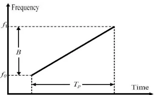
1. Linear Frequency Modulation: LFM modulation is most widely used mod-ulation technique in radar. In this method, the carrier frequency of sinusoidal is varied linearly with time. If the frequency of carrier increases linearly across the pulse, then it is known as up-chirp signal (shown in Figure 2.6), if frequency decreases then it is known as down-chirp signal. The instantaneous phase of chirp signal can be expressed as

ϕ(t) =2π(f0t+ 1 2kt

2₎ _(2.37)

where f₀ is frequency of the carrier. kis the rate of change of frequency. k is related to the bandwidthBand pulse duration Tp of pulse as

k= B Tp

(2.38)

(36)

Figure 2.6: The instantaneous frequency of the LFM waveform over time

The instantaneous frequency is given by [4, p. 58] f(t) = d dt(f0t+ 1 2kt 2_{) =} _f 0+kt (2.39)

LFM techniques increase the bandwidth of the signal thereby improving the range resolution by a factor equals to the time-bandwidth product [4, p. 61]. ACF of LFM signal shows high side lobes (−13.2 dB below the main lobe peak), [1, p. 343] which is not acceptable in certain radar applications where the number of targets are more than one that gives rise to echoes of different amplitudes. Some major techniques like time domain weighting, frequency domain weighting and NLFM are used to get lower side lobes level. The amplitude modulation of the transmitted signal is equivalent to time domain weighting that gives rise to low transmitted power thereby lowering the SNR. Frequency domain weighting broadens main lobe. NLFM overcomes the above two problems, and there is no mismatch loss [2, 5, 6].

2. Noninear Frequency Modulation: Despite having several advantages, the nonlinear-FM waveform has little acceptance. The waveform is designed in such a way that it provides the desired amplitude spectrum hence no time or frequency weighting is required in this NLFM waveform for range sidelobe

(37)

suppression. The matched filter output, when transmitted signal is an NLFM pulse, gives low side lobe levels. If a weighting is applied to the signal, the re-sultant loss in SNR can be overcome by the general mismatching techniques. The reduction in frequency side lobes by time weighting a symmetrical FM modulation gives rise to near-ideal ambiguity function [7]. The limitations of the NLFM waveform are listed as:

1. Using NLFM pulse increase the system complexity,

2. There is a very little development of NLFM generation equipments, 3. In NLFM pulse, for each amplitude spectrum, a separate FM modulation

design is required.

2.6 Simulation Results

In this section, we simulate the basic waveform used in radar and their ambi-guity function. Figure 2.7 and 2.8 shows the plot of LFM pulse. The bandwidth of LFM pulse is 200MHzand the pulse duration is 10µsec. Figure 2.7 shows the real part of the pulse and imaginary part of LFM pulse is shown in Figure 2.8. The spectrum of this LFM pulse is shown in Figure 2.9.

−1 −0.8 −0.6 −0.4 −0.2 0 0.2 0.4 0.6 0.8 1 x 10−6 −1 −0.8 −0.6 −0.4 −0.2 0 0.2 0.4 0.6 0.8 1 Time − seconds Amplitude

Real part of an LFM waveform

Figure 2.7: Real Part of LFM signal. B=200MHz,t=10µsec.

(38)

Chapter 2. Introduction −1 −0.8 −0.6 −0.4 −0.2 0 0.2 0.4 0.6 0.8 1 x 10−6 −1 −0.8 −0.6 −0.4 −0.2 0 0.2 0.4 0.6 0.8 1 Time − seconds Amplitude

Imaginary part of LFM waveform

Figure 2.8: Imaginary Part of LFM signal. B=200MHz,t =10µsec.

−5 −4 −3 −2 −1 0 1 2 3 4 5 x 108 0 50 100 150 200 250 300 Frequency − Hz Amplitude spectrum

Spectrum for an LFM waveform

(39)

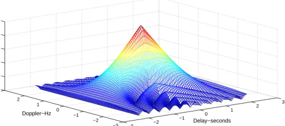
Chapter 2. Introduction −3 −2 −1 0 1 2 3 −3 −2 −1 0 1 2 3 0 0.2 0.4 0.6 0.8 1 Delay−seconds Doppler−Hz Ambiguity function

Figure 2.10: Ambiguity function plot of single pulse, constant frequency signal

Figure 2.11: Ambiguity function plot of single pulse, constant frequency signal for zero Doppler cut.

(40)

Chapter 2. Introduction −50 −4 −3 −2 −1 0 1 2 3 4 5 0.1 0.2 0.3 0.4 0.5 0.6 0.7 0.8 0.9 1 Frequency Ambiguity function

Figure 2.12: Ambiguity function plot of single pulse, constant frequency signal for zero delay cut.

−1.5 −1 −0.5 0 0.5 1 1.5 −10 −5 0 5 100 0.2 0.4 0.6 0.8 1 Delay−seconds Doppler−Hz Ambiguity function

(41)

Chapter 2. Introduction −1.50 −1 −0.5 0 0.5 1 1.5 0.1 0.2 0.3 0.4 0.5 0.6 0.7 0.8 0.9 1 frequency Ambiguity function

Figure 2.14: Ambiguity function plot of single LFM pulse zero Doppler cut

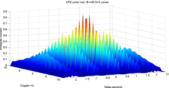
Figure 2.15: Ambiguity function plot for LFM pulse train. Number of pulseN=3

(42)

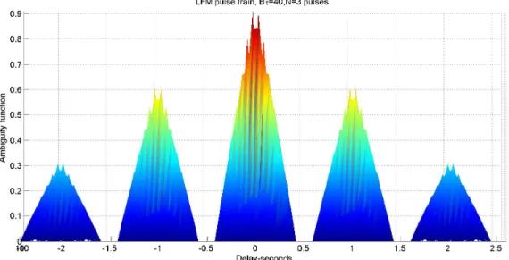
Figure 2.16: Ambiguity function plot for LFM pulse train for zero Doppler cut. Number of pulse N=3

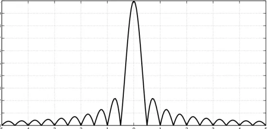
Figure 2.10 shows the ambiguity function plot of single, constant frequency pulse. In this ambiguity function no side lobes in time axis is visible. Some side lobes may be visible in Doppler axis. Figure 2.11 shows the plot of ambiguity function for zero Doppler cut. From this figure we can see that there are no side lobes present. So there is no uncertainty in detecting of the object. But the width of main lobe is very high, so the range resolution of this pulse is very poor. Figure 2.12 shows the plot of ambiguity function for zero delay cut. Here Doppler resolu-tion is good, so we can predict the frequency shift accurately (almost accurately), but because of side lobes there will always be some uncertainty.

Figure 2.13 shows the ambiguity function plot of single LFM pulse. This figure shows the side lobes in both Doppler and Time axis. For zero Doppler cut, the ambiguity function plot is shown in Figure 2.14. For single LFM pulse, the range resolutions improves as compare to the constant frequency pulse but because of the presence of side lobe, uncertainty in finding object increases. For zero delay cut, the uncertainty increases and the resolution decreases. Figure 2.15 and 2.16 shows the plot of ambiguity function for stepped frequency pulse train and its zero delay cut. Since each waveform in SFPT is processed separately, so we get improved range resolution and less uncertainty in detecting the target.

(43)

2.7 Conclusion

This chapter presents the basic concepts of pulse compression systems. First the pulse compression and need of pulse compression is explained in this chapter, then matched filter is explained. The derivation for the matched filter response of narrow band signal is done next. To compare the performance of different radar signal, the concept of ambiguity function is explained with its property. Phase and frequency modulated signal with their advantage and disadvantage is also dis-cussed. In last section MATLAB simulation of various radar signals is shown. In that section, we also shows and described the ambiguity function plot with their zero delay and Doppler cut. Based on the comparison of radar signal on the basis of ambiguity function we conclude that SFPT is better signal in terms of range resolution and uncertainty in object detection.

(44)

Chapter 3 Coherent Train of LFM Pulses

Introduction Analysis of Stepped Frequency Pulse Train Side lobe and Grating Lobe Sidelobe Reduction Grating lobe Reduction Problem Formulation for Optimization

(45)

Chapter 3 Coherent Train of LFM Pulses

3.1 Introduction

Range resolution is one of the very important property of radar signals. The range resolution depends upon the bandwidth of the radar signal. In fact, it is in-versely proportional to the bandwidth of the radar signal. If we increase the band-width of the signal, its range resolution will improve correspondingly. Improve-ment in range resolution is good for pulse compression system. Range resolution can be improved by using wide-band pulses, but bulky and costly transmitters and receivers are the drawbacks of using wide-band pulse. Also, other sources can cause interference to wide-band pulses. Another way to achieve wide-band pulse is to change linearly the center frequencies of the pulse train [8]. A fundamental waveform is used to modulate the each pulse of the pulse train. When we use LFM pulse to modulate pulse train, then the resultant signal is known as Stepped Fre-quency Pulse Train (SFPT) or Synthetic Wide-band Waveform (SWW). SFPT is a wide-band signal, but it can be used in the narrow-band transmitters and receivers. Using SFPT, in radar system, simplifies the design of the radar systems.

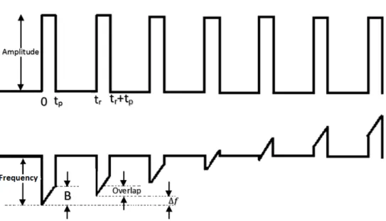
Figure 3.1 shows the frequency and amplitude plot for SFPT. Pulse train having N number of coherent pulses, duration of each pulse is Tp and repetition time is

Tr. The bandwidth of each pulse is B. ∆f is the frequency step between two

consecutive pulses. It is assume that Tp, Band ∆f remain constant throughout the

pulse. Also B>∆f >0.

(46)

Chapter 3. Coherent Train of LFM Pulses

Figure 3.1: Stepped Frequency Pulse Train

3.2 Analysis of Stepped Frequency Pulse Train

The complex envelope of a unmodulated pulse (constant frequency signal ) of durationTp is given by [p. 169] [9] u(t) = _p1 Tp rect t Tp (3.1)

Frequency modulation is applied to unmodulated pulse to get an LFM Signal. The complex envelope of LFM pulse is given by

u₁(t) = _p1 Tp rect t Tp exp jπkt2 (3.2)

k is the frequency slope. k is defined in terms of the bandwidth of single LFM pulse (B) and pulse duration(Tp) as

k=±B

Tp

(3.3) Here +and− signs are for positive and negative frequency slope respectively. In this analysis, positive value ofk is used but the analysis is equally valid for the negative value of k. Instantaneous frequency of LFM signal is given by

f(t) = 1 2π

d πkt2

dt (3.4)

(47)

Chapter 3. Coherent Train of LFM Pulses is expressed as uN(t) = 1 √ N N−1

∑

n=0 u₁(t−nTr) (3.5)

To maintain unit energy the multiplication factor √1

N is included in the

expres-sion. Further a slope of ks is applied to entire LFM pulse train. The complex

envelope of resultant signal is represented as

us(t) =uN(t)exp jπkst2 us(t) = 1 √ N exp jπkst2 N−1

∑

n=0 u₁(t−nTr) (3.6) where ks =± ∆f Tr ∆f >0 (3.7)

+and−signs stand for positive and negative frequency slope respectively. The overall bandwidth of SFPT is expressed as

BT = (k+ks)Tp∆f (3.8)

The ACF of us(t) is Obtained in [9] as |R(τ)|= 1−|τ| Tp sinc Bτ 1−|τ| Tp sin(Nπ τ∆f) Nsin(π τ∆f) (3.9)

The expression for |R(τ)| is product of two terms. First one is the ACF of single LFM pulse and is given by

|R1(τ)|= 1−|τ| Tp sinc Bτ 1−|τ| Tp (3.10) and the second term produces grating lobe in ACF of SFPT.

|R₂(τ)|= sin(Nπ τ∆f) Nsin(π τ∆f) τ ≤Tp (3.11)

3.3 Side lobe and Grating Lobe

Side lobe will result in the ambiguity function plot of signal when we try to squeeze the main lobe width. From the property of ambiguity function, if we try

(48)

Chapter 3. Coherent Train of LFM Pulses 0 0.1 0.2 0.3 0.4 0.5 0.6 0.7 0.8 0.9 1 0 0.2 0.4 0.6 0.8 1 τ /T_p |(R 1 ( τ ))|, |(R 2 ( τ ))| 0 0.1 0.2 0.3 0.4 0.5 0.6 0.7 0.8 0.9 1 −60 −40 −20 0 τ / T_p ACF in dB

Figure 3.2: SFPT forT_p∆f =3,TpB=4.5 andN=8. Top shows|R1(τ)|in solid line and|R2(τ)|

in dashed line. Bottom shows ACF in dB.

0 0.1 0.2 0.3 0.4 0.5 0.6 0.7 0.8 0.9 1 0 0.2 0.4 0.6 0.8 1 τ / T p |(R 1 ( τ ))|, |(R 2 ( τ ))| 0 0.1 0.2 0.3 0.4 0.5 0.6 0.7 0.8 0.9 1 −60 −40 −20 0 τ / T_p ACF in dB

Figure 3.3: Constant frequency pulse train forTp∆f =3,TpB=0 andN=8. Top shows|R1(τ)|

in solid line and|R₂(τ)|in dashed line. Bottom shows ACF in dB.

to reduce the main lobe width, then the volume must appear somewhere else. This volume appears near the main lobe width in the form of side lobes. The more we try to squeeze main lobe width, the more side lobes will appear.

Grating lobe is defined as the side lobe, which is having significant energy as compared to main lobe. The grating lobe are produced in ACF of radar signal because of the frequency overlap between two consecutive pulses. Grating lobe

(49)

appears when the product of pulse duration and frequency step become more than one (Tp∆f >1).

The ACF of SFPT is given in Equation 3.9. In this equation|R₁(τ)|is the ACF of single LFM pulse. |R₂(τ)|comes because ofN number of pulses used. |R2(τ)|, given by Equation 3.11, is responsible for producing the grating lobes.

Figure 3.2, 3.3 shows the plot of ACF of SFPT, for different values ofTp∆f and

TpB. Figure 3.2 shows the plot of ACF of SFPT for Tp∆f =3 and TpB =4.5. In

this figure, we can see that |R₂(τ)| exhibits grating lobe at location g/∆f. These

grating lobe have very low effect on the magnitude of ACF. The magnitude plot of |R(τ)| is also shown below. In the magnitude plot high side lobes can be seen near the main lobe. The peak side lobe level in this case is −13.2 dB below the main lobe.

Figure 3.2 shows the plot of ACF of constant frequency pulse train forTp∆f =3

and TpB=0. The magnitude plot of ACF shows grating lobe at location τ/Tp =

0.35 and at 0.65. The magnitude plot shows high side lobes and grating lobes. The amplitude of grating lobe is considerable. These grating can be misunderstood as a second target, so they are undesirable in the plot of ACF.

3.4 Side lobe Reduction

The matched filter response of LFM signal has very high peak side lobes (

−13.2 dB below the main lobe level). These high side lobes might not be ac-ceptable in some radar applications. These high side lobes might be mistaken for a target, or they may hide a weak target. Transmitting non-uniform amplitude pulse is one way to reduced these side lobes. This can be done by applying ampli-tude weighting over pulse duration Tr (also known as windowing). Unfortunately,

this method is not practical for high power radar. High power transmitter such as Traveling wave tubes, Klystrons should be operated saturated to obtain maximum efficiency. They can’t be operated with amplitude modulation. They should be operated in either full-on or full-off. Solid state transmitter can be amplitude mod-ulated because of linear input-output relation, provided that they are operating in

(50)

Table 3.1: Weighting function to reduce the side lobes

Weighting function Peak side lobe (dB) Loss (dB) Mainlobe width (relative)

Uniform −13.2 0 1.0 0.33+0.66cos2(πfB) −25.7 0.55 1.23 cos2(πfB) −31.7 1.76 1.65 0.16+0.84cos2(πfB) −34.0 1.0 1.4 Taylorn=6 −40.0 1.2 1.4 0.08+0.92cos2(πfB) −42.8 1.34 1.5

Class-A. Solid state transmitter always operates in Class-C because of the much higher efficiency of Class-C.

Another method of reduce the side lobe is by applying amplitude weighting at the receiver end. Since the filter used for pulse compression is matched filter, using amplitude weighting results in mismatch filter. This also results in a loss of SNR. Table 3.1 gives the example of weightings, the peak side lobe, and other properties of the output waveform.

The mismatched-filter loss can be kept to about 1 dB when the peak side lobe level is reduced to 30 dB below the main lobe level. Theoretically it is possible to have no loss in SNR and still achieve low side lobes with a uniform amplitude transmitter if nonlinear LFM is used.

3.5 Grating lobe Reduction

Different methods are given in literatures for complete rejection or acceptable suppress of grating lobes. In [10,11] the pulse width is varied to reduce the grating lobes but varying pulse width destroys the periodicity of the pulse train. A method describes in [12] for grating lobe suppression. In this method energy of pulse train is distributed non-uniformly over the desired frequency band to get reduced grat-ing lobe, higher range resolution and lower range side lobes, but spectral weight-ing applied for non-uniform distribution of energy, introduces additional losses in sensitivity. In [9], Levanon and Mozeson have given a relationship for Tp∆f,TpB

and B/∆f. If the parameter of SFPT satisfy this relation then we can completely

(51)

nullifying first two grating lobe results in nullification of all the grating lobes. To establish such a relation between parameters of SFPT is too difficult, also in this approachN should be large if we want a significant increase in bandwidth. In [13] the grating lobes are reduced to an acceptable level by forcing the ampli-tude of ACF of a single frequency LFM pulse, below a predefined level at the loca-tion of grating lobe. The above menloca-tioned approach does not reduce the range side lobe that occur near the main lobe. Non-Linear Frequency Modulated (NLFM) is used instead of LFM pulse for suppression of range side lobe but NLFM wave-forms are not Doppler tolerant. A Multi-Objective Optimization (MOO) technique (Nondominated Sorting Genetic Algorithm (NSGA-II) [14]) is used by Sahoo and Panda [15] to find the parameter of SFPT for side lobes and grating lobes suppres-sion. The complexity of the algorithm is O(MN2). M is the number of objective function used for optimization and N is the number of solution used in optimiza-tion process. In search of better Pareto front and reduced complexity, Kumar and Sahoo in [16] used Multi Objective Particle Swarm Optimization (MOPSO) [17] algorithm. This algorithm has computational complexity of O(MN). This works gives the lower peak side lobe for a particular grating lobe amplitude.

3.6 Problem Formulation for Optimization

The grating lobe and side lobes affects the range resolution of SFPT and may hide weak targets. so it is required to suppress or nullify these grating lobes and range side lobes. In this work, the minimization of grating lobe and side lobe has been studied in two different way, which are as follow.

3.6.1 Problem Formulation-1

In the output of matched filter the maximum side lobe level should be low as compare to main lobe level. To minimize the side lobe level Peak to Sidelobe Ratio (PSR) is used as a objective function. PSR is defined in [15] as

PSR= Maximum sidelobe level in ACF

mainlobe level (3.12)

Also for grating lobe suppression the function defined in equation 3.10 should

(52)

be minimum or zero at τ =τg (grating lobe location). To have a meaningful

im-provement in range resolution the bandwidth of SFPT must be more than that of LFM pulse i.e. N∆f >B.

From equation 3.9, 3.10 and 3.11, we observed that ACF, |R₁(τ)| and |R2(τ)| are function of Tp∆f and TpB only for a given value of N. If we choose suitable

value of Tp∆f and TpB then grating lobe as well as side lobe can be minimized.

TpBis chosen by the following expression

TpB= (c+1)Tp∆f (3.13)

c is a positive number to ensure B>∆f. A positive value of censure that there

will be some overlap in frequency of consecutive pulse. Based on the discussion above, the objective functions, for optimization, can be formulate as [15]

Minimize f₁ =maxR₁(τ_g) where g =1,2, ...Tp∆f Minimize f₂ =PSR in dB

Sub jected to the constraints NTp∆f >TpB

3.6.2 Problem Formulation-2

The main lobe width depend upon the first overall null of the expression|R₁(τ)|

and |R₂(τ)|. The first null of |R₂(τ)| occurs at _NT1

p∆f and the first null of |R1(τ)|

occurs at _TpB1 approximately, if TpB>> 1. So the location of first overall null of

ACF is given by|R₂(τ)|, which is equal to τ₁st null Tp =min 1 TpB , 1 NTp∆f (3.14) under the assumption that TpB >> 1, the width of delay resolution depends on |R₂(τ)|, which is equal to _NT1

p∆f. In literature some weighting methods available,

which can be used to reduce the side lobes of an LFM pulse. By using weighting techniques, we emphasize centre frequency more as compare to end frequencies, which result in suppressed side lobe and widened main lobe. Wide main lobe decreases the range resolution. This outcome is also applicable for SFPT as we have used the conditionB>∆f >0.

(53)

In this problem we uses an objective of minimization of main lobe width. The other objective is minimization in PSR, which is same as problem-1. To ensure that grating lobes are suppressed, we add a constraint. This constraint ensure that maximum grating lobe amplitude is below a predefined level. Another constraint is added to ensure that bandwidth of SFPT is more than LFM pulse i.e. there will be some overlap in frequency. The objective functions for this problem, are as follow:

Minimize f₁ = 1 NTp∆f

Minimize f₂ =PSR in dB Sub jected to the constraints NTp∆f >TpB R₁(τ_g) <ε

3.7 Conclusion

This chapter gives us the basic understanding of coherent train of LFM pulses, also known as stepped frequency pulse train. In this chapter, first we derive the expression for ACF of SFPT. From the expression of ACF side lobes and grating lobe are explained. Then the techniques available in literature to suppress side lobe and grating lobe is discussed. By combining the side lobe and grating lobe suppression techniques we formulate two problems, which can be used to suppress both side lobe and grating lobe.

(54)

Chapter 4 Multi-Objective Optimization

Introduction Definitions NSGA-II IDEA MOPSO Performance Comparison Matrices Performance Comparison of MOO Algorithms Simulation Results Conclusion

(55)

Chapter 4 Multi-Objective Optimization Techniques

4.1 Introduction

In single-objective optimization problems, we want to find the best solution of the problem which is mostly the minimum or maximum value of the objective function. In practice, the optimization problem have many objective functions. The objective functions mostly are conflicting in nature. In this type of problem, we might not have one minimum or maximum solution, which is valid for all the objective functions. In MOO problem, there exists a set of solutions that are better than the other solutions for all the objective functions, but they are equally better among themselves. such solutions are called nondominated solutions or Pareto optimal solutions. Every solution in nondomination set is an acceptable solution. With the help of extra information about the objective function, we can find dominance of one solution over the others. The MOO algorithms used are described in Section 4.3, 4.4 and 4.5. The basics concepts of MOO are described below.

4.2 Definitions

To explain the multi-objective optimization techniques, and to understand the result, some non-ambiguous definitions are required. These definitions are pre-sented in this section.

(56)

Chapter 4. Multi-Objective Optimization Techniques

4.2.1 Single Objective Optimization

When the optimization problem only have one objective function than opti-mization of such function is known as “single objective optiopti-mization”. Generally in single objective optimization problem, we find the minimum value of the ob-jective function. For optimization of maximization problem, first the problem is changed to the minimization type problem.

4.2.2 Multi-Objective Optimization

In Multi-Objective Optimization (MOO) problem, we have more than one ob-jective function to simultaneously optimized under some constraints. In MOO problem, we search for a set of solutions (decision variable) which satisfies the constraints and gives the optimum value of objective functions. The objective functions generally conflict with each other. Hence, our aims is to find a set of solutions, which are nondominated with respect to each other, and can optimized (minimize) the objective functions. The MOO problem can be written as:

Minimize f1(x), ..., fk(x)

Sub ject to gi(x)> 0, i=1, ...,m

(4.1)

4.2.3 Pareto Optimality

A solution~x∗ ∈ Ω is said to be Pareto optimal if for every ~x ∈ Ω and I =

{1,2, ...k}either

∀_i∈I(fi(~x) = fi(~x∗)) (4.2)

or, there is at least onei∈I such that

fi(~x)> fi(~x∗) (4.3)

In other words, a solution is Pareto optimal, when there are no other feasible solution, in a set of solutions, which gives decrease in one objective function, without increasing one or more objective functions values.

(57)

4.2.4 Pareto Dominance

A solution ~u is aid to dominate ~v, if and only if ~u is partial less than ~v,i.e.

∀i∈ {1,2, ...k},ui ≤vi∧ ∃i∈ {1,2, ...k}:ui<vi.

In simple words a solution u is said to be dominate another solution v in a solution set, when the value of objective functions is equal for solution u and v and for at least one solution objective function value ofuis better than v.

4.3 Nondominated Sorting Genetic Algorithm-II

Nondominated Sorting Genetic Algorithm-II (NSGA-II) is a MOO algorithm, proposed by Deb in [14]. This work is an expansion of original NSGA algorithm given in [18]. Original NSGA was criticized because of its high computational complexityO MN3. Also, we have to specify a sharing parameter, and there was no method to preserve the elitism. NSGA-II employs a fast nondomination sorting method. The computational complexity of new approach is O MN2, where M is the number of objective function used for optimization andN is the population size. A selection operator is also used in this algorithm. Work of selection operator is to creates a mating pool. In mating pool, we combines the child and parent populations and select the best member for the new generation (with respect to objective function and crowding distance). Elitism is ensured by combining the child population with parent population. The working of this algorithm can be divided into three parts.

A. Fast Nondominated Sorting Approach

Let the population size is N. For fast nondomination sorting approach, we calculate two entities for each member of the population:

1. domination countnp, the number of solution that dominates the solution p.

2. Sp a set of solution, that solution pdominates.

The solutions that have their domination count as zero, we place them in first nondomination front. Now for each member p of first nondomination front,

(58)

Algorithm 1Nondominated Sorting Genetic Algorithm-II

Required: N (Population size)

Required: gen(Number of generation)

1: InitializeParent Population

2: Evaluate objective function

3: Apply nondominated sorting and crowding distance assignment

4: fori=1:gendo

5: Apply tournament selection

6: Apply crossover and mutation to generate offspring population

7: Evaluate objective function for offspring population

8: Combine parent and offspring population

9: Apply nondominated sorting and crowding distance assignment to combined population

10: SelectNfeasible individuals

11: end for

we visit every member qof its set Sq and reduce the domination count of qby

one. In doing this, if the domination count of a solution become zero, we put that solution to next domination level. Now, the above process is continued with the next domination level. We repeat this process until all This solutions are placed in a nondomination front.

The domination count np of a solution available in second or higher

nondom-ination front, can maximum be N −1. So, a solution p will be accessed by at most N−1 times before its domination counts turns into zero. When the domination count of a solution become zero, we assign a nondomination level to that solution and will not access that solution any further. Since there are at mostN−1 such solutions, the aggregate complexity isO N2. Therefore, the general complexity of the system isO MN2.

B. Diversity Preservation

Diversity preservation is used, so that the obtain Pareto front maintain an ex-cellent spread of the solutions. In original NSGA, we need to specify a sharing function for diversity preservation. In this algorithm sharing function approach is replaced by a crowd comparison method. In this approach, we first estimate the density, then we apply crowd comparison operator.

(59)

Figure 4.1: Crowding distance calculation

specific solution. We calculate the average distance (i_distance) of solutions surrounding the solution on either side of this solutions along each of the destinations. Figure 4.1 shows the solution in the front with solid circles. To calculate crowding distance for solution i, we form a cuboid between solution i+1 and i−1 (dashed box). The crowding distance for solution i is the average length of side in the cuboid.

To analyze solutions on the basis of crowding distance, we first sort the pop-ulation in rising order of objective function value. The boundary solutions, for each objective functions, are assigned a distance value of infinite. To assigned distance value to Solutions in between the boundary solutions, we calculate, for two adjacent solutions, the absolute normalized difference of objective function values. For each objective function, we repeat this pro-cedure. The sum of all the distance calculated for a solution is known as the crowding distance. Before calculating crowding distance, we first normal-ized the objective function value.

2. Crowed-Comparison Operator: The crowd comparison operator is de-noted by≺_n. It guides the selection process to a uniform spread-out Pareto optimal front. We assume that every solutioniis having two attributes: a. Nondomination rank (irank);

(60)

b. Crowding distance (idistance).

we now define a partial operator≺_n as

i≺nj i f(irank < jrank)

or ((i_rank= jrank)

and (i_dis_tan_ce> j_dis_tan_ce))

(4.4)

In crowd comparison, we prefer the solution that is in lower nondomination front. If both solutions are in same nondomination front, then we chose solution whose distance metric is large means solution located in the lesser crowded area.

C. Main Loop

In this algorithm, for the very first generation, we create a random population P₀ of size N. Then we apply nondomination sorting on the population and assign a rank (equal to its nondomination level) to each solution. At first, the binary tournament is chosen to select the parent for crossover and mutation operator. Simulated binary operator is used for crossover. This operation gives us child population Q₀ of size N. Now we combine the child population with parent population. Elitism is introduced in this algorithm by comparing current population with previously found best-nondominated solutions, the procedure is different after the initial generation. The tth generation of this algorithm is shown in Figure 4.2.

Fortth generation the combined population is denoted asRt =Pt∪Rt.The size

of Rt is 2N. The population Rt is sorted based on nondomination criterion.

Since all previous and current population members are included in Rt, elitism

is ensured. Now, the solutions in first nondomination front F₁ are the best so-lutions of the total population, so we prefer the solution of first nondomination front. If the total number of solution in first nondomination front is less than N, then we choose all the solution of first front for new population pt+1. The remaining members of the population pt+1 are chosen from subsequent non-dominated fronts in the order of their ranking. Thus, solutions from the setF₂

(61)

Figure 4.2: NSGA-II procedure

are chosen next, followed by solutions from the set F₃, and so on. We repeat this procedure until we are unable to accommodate the next front. Let’s say that the set Fl is the last nondominated set beyond which no other set can be

accommodated. The total number of solutions from F₁ to Fl is more than N.

To accommodate exactly N number of solution in Pt+1, we choose remaining solution from Fl. we sort the solutions of the last frontFl using the

crowded-comparison operator ≺_n in descending order and choose the best solutions needed to fill all population slots.

The new population Pt+1 of size N is now used for selection, crossover, and mutation to create a new child population Qt+1. NSGA-II use binary tour-nament selection operator but the selection criterion is based on crowded-comparison operator ≺n.

RADAR Signal Processing Using Multi-Objective Optimization Techniques

RADAR Signal Processing using

Multi-Objective Optimization Techniques

Vinod Kumar

RADAR Signal Processing using

Multi-Objective Optimization Techniques

Master of Technology

Signal & Image Processing

Vinod Kumar

Prof. Ajit Kumar Sahoo

National Institute of Technology

Rourkela

National Institute of Technology

Rourkela

Acknowledgment

Abstract

Contents

List of Figures

List of Tables

List of Algorithms

List of Acronyms

Acronym

Description

ACF

Autocorrelation Function

AF

Ambiguity Function

AWGN

Additive White Gaussian Noise

BW

Bandwidth

IDEA

Infeasibility Driven Evolutionary Algorithm

CW

Continuous Wave

LFM

Linear Frequency Modulation

NSGA

Nondominated Sorting Genetic Algorithm

MOO

Multi-Objective Optimization

MOPSO

Multi-Objective Particle Swarm Optimization

PCR

Pulse Compression Ratio

PSD

Power Spectral Density

PSO

Particle Swarm Optimization

PSR

Peak to Side lobe Ratio

RADAR

Radio Detection and Ranging

SFPT

Stepped Frequency Pulse Train

SNR

Signal to Noise Ratio

Chapter 1

Thesis Overview

Chapter 1

Thesis Overview

1.1

Background

1.2

Motivation

1.3

Objective

1.4

Thesis Organization

Chapter 2

Introduction

Chapter 2

Introduction

2.1

Introduction

2.2

Pulse Compression

2.3

Matched Filter

2.4