Bayesian Dynamic Tensor Regression
∗Monica Billio†1, Roberto Casarin‡1, Sylvia Kaufmann§2, Matteo Iacopini¶1,3 1Ca’ Foscari University of Venice
2Study Center Gerzensee, Foundation of the Swiss National Bank 3Université Paris I - Panthéon-Sorbonne
May 8, 2018
Abstract
Multidimensional arrays (i.e. tensors) of data are becoming increasingly available and call for suitable econometric tools. We propose a new dynamic linear regression model for tensor-valued response variables and covariates that encompasses some well known multi-variate models such as SUR, VAR, VECM, panel VAR and matrix regression models as special cases. For dealing with the over-parametrization and over-fitting issues due to the curse of dimensionality, we exploit a suitable parametrization based on the parallel factor (PARAFAC) decomposition which enables to achieve both parameter parsimony and to in-corporate sparsity effects. Our contribution is twofold: first, we provide an extension of multivariate econometric models to account for both tensor-variate response and covariates; second, we show the effectiveness of proposed methodology in defining an autoregressive process for time-varying real economic networks. Inference is carried out in the Bayesian framework combined with Monte Carlo Markov Chain (MCMC). We show the efficiency of the MCMC procedure on simulated datasets, with different size of the response and indepen-dent variables, proving computational efficiency even with high-dimensions of the parameter space. Finally, we apply the model for studying the temporal evolution of real economic networks.
∗
We thank the conference, workshop and seminar participants at: “CFENetwork 2017” in London, “ESOBE 2016” in Venice, “CFENetwork 2016” in Seville, “ICEEE 2017” in Messina of the Italian Econometric Society, the “3rd Vienna Workshop on High-dimensional Time Series in Macroeconomics and Finance”, “BISP10” at Bocconi University of Milan and the “SIS Intermediate Meeting” of the Italian Statistical Society in Florence. Iacopini’s research is supported by the “Bando Vinci 2016” grant by the Université Franco-Italienne. This research used the SCSCF multiprocessor cluster system at Ca’ Foscari University of Venice.
† e-mail: [email protected] ‡ e-mail: [email protected] § e-mail: [email protected] ¶ e-mail: [email protected]
1
Introduction
The increasing availability of large sets of time series data with complex structure, such as EEG (e.g., Li and Zhang (2017)), neuroimaging (e.g., Zhou et al. (2013)), two or multidimensional tables (e.g., ,Balazsi et al. (2015), Carvalho and West (2007)), multilayer networks (e.g., Alda-soro and Alves (2016), Poledna et al. (2015)) has put forward some limitations of the existing
multivariate econometric models. In the era of “Big Data”, mathematical representations of
information in terms of vectors and matrices have some non-negligible drawbacks, the most re-markable being the difficulty of accounting for the structure of the data, their nature and the way they are collected (e.g., contiguous pixels in an image, cells of matrix representing a geographical map). As such, if this information is neglected in the modelling the econometric analysis might provide misleading results.
When the data are gathered in the form of matrices (i.e. 2-dimensional arrays), or more generally as tensors, that is multi-dimensional arrays, a statistical modelling approach can rely on vectorizing the object of interest by stacking all its elements in a column vector, then resorting to standard multivariate analysis techniques. The vectorization of an array does not preserve the structural information encrypted in its original format. In other words, the physical char-acteristics of the data (e.g, the number of dimensions and the length of each of them) matter, since a cell is highly likely to depend on a subset of its contiguous cells. Collapsing the data into a 1-dimensional array does not allow to preserve this kind of information, thus making this sta-tistical approach unsuited for modelling tensors. The development of novel methods capable to deal with 2- or multi-dimensional arrays avoiding their vectorization is still an open challenging question in statistics and econometrics.
Many results for 1-dimensional random variables in the exponential families have been ex-tended to the 2-dimensional case (i.e. matrix-variate, see Gupta and Nagar (1999) for a com-pelling review). Conversely, tensors have been recently introduced in statistics (see Hackbusch (2012), Kroonenberg (2008), Cichocki et al. (2009)), providing the background for more efficient
algorithms in high dimensions especially in handling Big Data (e.g. Cichocki (2014)). However,
a compelling statistical approach to multi-dimensional random objects is lacking and constitutes a promising field of research.
Recently, the availability of 3-dimensional datasets (e.g., medical data) has fostered the use of tensors in many different fields of theoretical and applied statistics. The main purpose of this article is to contribute to this growing literature by proposing an extension of standard multivariate econometric models to tensor-variate response and covariates.
Matrix models in econometrics have been employed over the past decade, especially in time series analysis where they have been widely used for providing a state space representation (see Harrison and West (1999)). However, only recently the attention of the academic community has moved towards the study of this class of models. Within the time series analysis literature, matrix-variate models have been used for defining dynamic linear models (e.g., Carvalho and West (2007) and Wang and West (2009)), whereas Carvalho et al. (2007) exploited Gaussian graphical models for studying matrix-variate time series. In a different context, matrix models have also been used for classification of longitudinal datasets in Viroli (2011) and Viroli and Anderlucci (2013).
Viroli (2012) the author presented a first generalization of the multivariate regression by in-troducing a matrix-variate regression where both response and covariate are matrices. Ding and Cook (2016) propose a bilinear multiplicative matrix regression model whose vectorisewd form
is a VAR(1) with restrictions on the covariance matrix. The main shortcoming in using bilinear
models (either in the additive or multiplicative form) is the difficulty in introducing sparsity constrains. Imposing a zero restriction on a subset of the reduced form coefficients implies a
zero restriction on the structural coefficients1. Ding and Cook (2016) proposed a generalization
of the envelope method of Cook et al. (2010) for achieving sparsity and increasing efficiency of the regression. Further studies which have used matrices as either the response or a covariate include Durante and Dunson (2014), who considered tensors and Bayesian nonparametric frame-works and Hung and Wang (2013), who defined a logistic regression model with a matrix-valued covariate.
Following the model specification strategy available in the existing literature, there are two main research streams. In the first one, Zhou et al. (2013), Zhang et al. (2014) and Xu et al.
(2013) propose a linear regression models with a real-valuedN-order tensorX of data to explain
a one-dimensional response, by means of the scalar product with a tensor of coefficients Bof the
same size. More in detail, Zhang et al. (2014) propose a multivariate model with tensor covariate for longitudinal data analysis; whereas Zhou et al. (2013) uses a generalized linear model with exponential link and tensor covariate for analysing image data. Finally, the approach of Xu et al. (2013) exploits a logistic link function with a tensor covariate to predict a binary scalar response. In the second and more general stream of the literature (e.g., Hoff (2015) and Li and Zhang (2017)) both response and covariate of a regression model are tensor-valued. From a modelling
point of view, there are different strategies. Hoff (2015) regresses a N-order array on an array
of the same order but with smaller dimensions by exploiting the Tucker product, and follows the Bayesian approach for the estimation. Furthermore, Bayesian nonparametric approaches for models with a tensor covariate have been formulated by Zhao et al. (2013), Zhao et al. (2014) and Imaizumi and Hayashi (2016). They exploited Gaussian processes with a suitable covariance kernel for regressing a scalar on a multidimensional data array. Conversely, Li and Zhang (2017) defines a model where response and covariates are multidimensional arrays of possibly different order, and subsequently uses the envelope method coupled with an iterative maximum likelihood method for inference.
We propose a new dynamic linear regression modelling framework for tensor-valued response and covariates. We show that our framework admits as special cases Bayesian VAR models (Sims and Zha (1998)), Bayesian panel VAR models (proposed by Canova and Ciccarelli (2004), see Canova and Ciccarelli (2013) for a review) and Multivariate Autoregressive models (i.e. MAR, see Carriero et al. (2016)), as well as univariate and matrix regression models. Furthermore, we exploit the PARAFAC decomposition for reducing the number of parameters to estimate, thus making inference on network models feasible.
We also contribute to the empirical analysis of tensor data in two ways. First, we provide an original study of time-varying economic and financial networks and show that our model can be succesfsfully used to carry out forecast and impulse response analysis in this high-dimensional stting. Few attempts have been made to model time-evolving networks (for example, Holme and Saramäki (2012), Kostakos (2009), Barrat et al. (2013), Anacleto and Queen (2017) and references in Holme and Saramäki (2013)), and this field of research, which stems from physics, has focused on providing a representation and a description of temporally evolving graphs. Second, we show how tensor regression con be applied to macroeconomic panel data, where standard vectorized models cannot be used.
The structure of the paper is as follows. Section 2 is devoted to a brief introduction to tensor calculus and to the presentation of the new modelling framework. The details of the estimation procedure are given in Section 3. In Section 4 we test proposed model on simulated datasets and in Section 5 we present some empirical applications.
1The phenomenon is worse in the bilinear multiplicative model, given that each reduced form coefficient is given by the product of those in the structural equation.
2
A Tensor Regression Model
We introduce multi-dimensional arrays (i.e. tensors) and some basic notions of tensor algebra which will be used in this paper. Moreover, we present a general tensor regression model and discuss some special cases.
2.1 Tensor Calculus and Decompositions
The use of tensors is well established in physics and mechanics (see Synge and Schild (1969), Adler et al. (1975), Malvern (1986), Lovelock and Rund (1989), Aris (2012) and Abraham et al. (2012)), but very few references can be found in the literature outside these disciplines. For a general introduction to the algebraic properties of tensor spaces we refer to Hackbusch (2012). A note-worthy introduction to tensors and corresponding operations is in Lee and Cichocki (2016), while we make reference to Kolda and Bader (2009) and Cichocki et al. (2009) for a review on tensor decompositions. In the rest of the paper we will use the terms tensor decomposition and tensor representation interchangeably, even though the latter one is more suited to our approach.
A N-order tensor is a N-dimensional array (whose dimensions are also called modes). The
number of dimensions is the order of the tensor. Vectors and matrices are examples of first- and
second-order tensors, respectively, while one may think about a third order tensor as a series of matrices of the same size put one in front of the other one, forming a parallelepiped. In the rest of the paper we will use lower-case letters for scalars, lower-case bold letters for vectors, capital letters for matrices and calligraphic capital letters for tensors. When dealing with matrices,
in order to select a column (or row) we adopt the symbol “:”. The same convention is used
for tensors when considering all elements of a given mode. For example, let A ∈ Rm×n be a
matrix and B ∈RI1×...×IN an array of orderN, thenA
i,j and Bi1,...,iN indicate the (i, j)-th and
(i1, . . . , iN)-th element of Aand B, respectively, and:
(i) A(i,:) is thei-th row ofA,∀i∈ {1, . . . , m};
(ii) A(:,j) is the j-th column of A,∀j ∈ {1, . . . , n};
(iii) B(i1,...,i
k−1,:,ik+1,...,iN) is the mode-kfiber ofB,∀k∈ {1, . . . , N}
(iv) B(i1,...,ik−1,:,:,ik+2,...,iN) is the mode-k, k+ 1slice of B,∀k∈ {1, . . . , N−1}
The mode-k fiber is the equivalent of rows and columns in a matrix, more precisely it is the
vector obtained by fixing all but thek-th index of the tensor. Instead, slices (i.e. bi-dimensional
fibers of matrices) or generalizations of them, by keeping fixed all but two or more dimensions (or modes) of the tensor.
Themode-nmatricization (or unfolding), denoted byX(n), is the operation of transforming
a N-dimensional array X into a matrix. It consists in re-arranging the mode-n fibers of the
tensor to be the columns of the matrixX(n), which has sizeIn×I¯(−n)withI¯(−n) =
Q
i6=nIi. The
mode-n matricization of X maps the (i1, . . . , iN) element of X to the (in, j) element of X(n),
where: j = 1 + X m6=n (im−1) m−1 Y p6=n Ip (1)
For some numerical examples, see Kolda and Bader (2009) and Appendix A. The mode-1
un-folding is of interest for providing a visual representation of a tensor: for example, whenX be a
third-order tensor, its mode-1unfoldingX(1)is a matrix of sizeI1×I2I3obtained by horizontally
stacking the frontal slices of the tensor. The vectorization operator stacks all the elements in
direct lexicographic order, forming a vector of length I¯ = Q
orderings are possible (as for the vectorisation of matrices), since the ordering of the elements is
not important as long as it is consistent across the calculations. The mode-n matricization can
also be used to vectorize a tensorX, by exploiting this relationship:
vec (X) = vecX(1)
, (2)
where vecX(1) stacks vertically into a vector the columns of he matrix X(1). Many product
operations have been defined for tensors (e.g., see Lee and Cichocki (2016)), but here we constrain
ourselves to the operators used in this work. Concerning the basic product operations, thescalar
product between two tensorsX,Y of equal order and same dimensions, I1, . . . , IN, is defined as:
hX,Yi= I1 X i1=1 . . . IN X iN=1 Xi1,...,iNYi1,...,iN = X i1,...,iN Xi1,...,iNYi1,...,iN. (3)
For the ease of notation, we will use the multiple-index summation for indicating the sum over all the corresponding indices.
The mode-M contracted product of two tensors X ∈ RI1×...×IM and Y ∈
RJ1×...×JN with
IM =JM, denoted X ×M Y, yields a tensor Z ∈ RI1×...×IM−1×J1×...×JN−1 of orderM +N −2,
with entries: Zi1,...,iM−1,j1,...,jN−1 = (X × M Y) i1,...,iM−1,j1,...,jN−1 = IM X iM=1 Xi1,...,iMYj1,...,iM,...,jN. (4)
Therefore, it is a generalization of the matrix product. The notation×1...M is used to denote a
sequence of mode-m contracted products, withm= 1, . . . , M.
Themode-nproduct between a tensor X ∈RI1×...×IN and a matrix A∈RJ×In,1≤n≤N,
is denoted byXׯnAand yields a tensorY ∈RI1×...,In−i,J,In+1,...×IN of the same order ofX, with
then-th mode’s length changed. Each mode-nfiber of the tensor is multiplied by the matrixA,
which yields element-wise:
Yi1,...,in−1,j,in+1,...,iN = (XׯnA)i
1,...,in−1,j,in+1,...,iN =
In X
in=1
Xi1,...,iNAj,in. (5)
Analogously, the mode-n product between a tensor and a vector, i.e. between X and v ∈ RIn,
yields a lower order tensor, since the n-th mode is suppressed as a consequence of the product.
It is given, element-wise, by:
Yi1,...,in−1,in+1,...,iN = (X ×nv)i 1,...,in−1,in+1,...,iN = In X in=1 Xi1,...,in,...,iNvin, (6)
with Y ∈RI1×...,In−i,In+1,...×IN. It is clear that, as for the matrix dot product, the order of the
elements in the multiplication matters and both products are not commutative.
TheHadamard product is defined in the same usual way as for matrices, i.e. the
element-wise multiplication. Formally, for X ∈RI1×...×IN,Y ∈
RI1×...×IN andZ ∈RI
×
1...×IN it holds:
Zi1,...,iN = (X Y)i1,...,iN =Xi1,...,iNYi1,...,iN. (7)
Finally, let X ∈RI1×...×IM and Y ∈RJ1×...×JN. Theouter product ◦of two tensors is the tensor
Z ∈RI1×...×IM×J1×...×JN whose entries are:
Zi1,...,iM,j1,...,jN = (X ◦ Y)i1,...,iM,j1,...,jN =Xi1,...,iMYj1,...,jN. (8)
For example, the outer product of two vectors is a matrix, while the outer product of two matrices is a fourth order tensor.
Tensor decompositions represent the core of current statistical models dealing with multi-dimensional variables since many of them allow to represent a tensor as a function of lower dimensional variables, such as matrices of vectors, linked by suitable multidimensional opera-tions. We now define two tensor decompositions, the Tucker and the parallel factor (PARAFAC), which are useful in our applications because the elements of the decomposition are generally low
dimensional and easier to handle than the original tensor. Let R be the rank of the tensor X,
that is minimum number of rank-1 tensors whose linear combination yieldsX. AN-order tensor
is of rank 1 when it is the outer product ofN vectors.
The Tucker decomposition is a higher-order generalization of the Principal Component
Anal-ysis (PCA): a tensor B ∈ RI1×...×IN is decomposed into the product (along the corresponding
modes) of a “core” tensorG ∈Rg1×...×gN and N factor matrices A(m) ∈
RIm×Jm,m= 1, . . . , N: B=G ×1A(1)×2A(2)×3. . .×NA(N)= g1 X i1=1 g2 X i2=1 . . . gN X iN=1 Gi1,i2,...,iNa(1)i 1 ◦a (2) i2 ◦. . .◦a (N) iN , (9) wherea(im) l ∈R
gm is the m-th column of the matrixA(m). As a result, each entry of the tensor
is obtained as: Bj1,...,jN = g1 X i1=1 g2 X i2=1 . . . gN X iN=1 Gi1,i2,...,iN ·A(1)i 1,j1· · ·A (N) iN,jN jm= 1, . . . , Im, m= 1, . . . , N . (10)
A special case of the Tucker decomposition, called PARAFAC(R)2, is obtained when the core
tensor is the identity tensor and the factor matrices have all the same number of columns,R. A
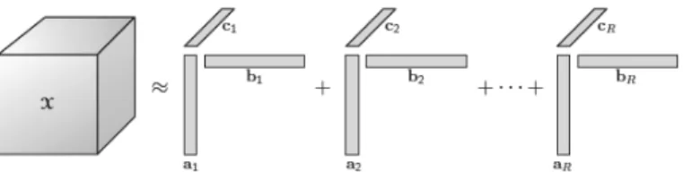
graphical representation of this decomposition for a third-order tensor is shown in Fig. (1). More
precisely, the PARAFAC(R) is a low rank decomposition which represents a tensorB ∈RI1×...×IN
as a finite sum of R rank-1 tensors obtained as the outer products of N vectors, also called
PARAFAC marginals3 β(jr)∈RIj,j = 1, . . . , N: B= R X r=1 Br = R X r=1 β(1r)◦. . .◦β(Nr). (11)
Remark 2.1. There exists a one-to-one relation between the mode-n product between a tensor and a vector and the vectorisation and matricization operators. Consider a N-order tensor
B ∈ RI1×...×IN for which is specified a PARAFAC(R) decomposition, a (N −1)-order tensor
Y ∈RI1×...×IN−1 and a vector x∈
RIN. Then:
Y =B ×Nx ⇐⇒ vec (Y) =B0(N)x ⇐⇒ vec (Y) 0
=x0B(N) (12)
and, denoting β(jr), for j = 1, . . . , N and r = 1, . . . , R, the marginals of the PARAFAC(R) decomposition of B we have: B(N) = R X r=1 β(Nr)vecβ(1r)◦. . .◦β(N−r)10 . (13)
2See Harshman (1970). Some authors (e.g. Carroll and Chang (1970) and Kiers (2000)) use the term CODE-COMP or CP instead of PARAFAC.
3An alternative representation may be used, if all the vectorsβr
j are normalized to have unitary length. In
this case the weight of each componentris captured by ther-th component of the vectorλ∈RR:
B= R X r=1 λr β(1r)◦. . .◦β(Nr) .
Figure 1: PARAFAC decomposition of X ∈RI1×I2×I3, with ar ∈ RI1, br ∈
RI2 and cr∈RI3,r = 1, . . . , R. Figure from Kolda and Bader (2009).
These relations allows to establish a link between operators defined on tensors and operators defined on matrices, for which plenty of properties are known from linear algebra.
Remark 2.2. For two vectorsu∈Rnandv∈
Rm the following relations hold between the outer
product, the Kronecker product ⊗and the vectorisation operator:
u⊗v0 =u◦v=uv0 (14)
u⊗v= vec (v◦u) . (15)
2.2 A General Dynamic Model
The new model we propose, in its most general formulation is:
Yt=A0+ p X j=1 Aj×N+1vec Yt−j+B ×N+1vec (Xt) +C ×N+1zt+D ×nWt+Et, (16) Etiid∼ NI1,...,IN(0,Σ1, . . . ,ΣN),
where the tensor response and noise Yt,Et areN-order tensors of sizes I1×. . .×IN, while the
covariates include a M-order tensor Xt of sizes J1 ×. . .×JM, a matrix Wt with dimensions
In×K and a vectorzt of lengthQ.
The coefficients are all tensors of suitable order and sizes: Aj have dimensionsI1×. . .×IN×I∗,
with I∗ = Q
iIi, B has dimensions I1 ×. . .×IN ×J∗, with J∗ =
Q
jJj, C has dimensions
I1×. . .×IN ×Q and D has sizes I1×. . .×In−1×K×In+1. . .×IN. The symbol×n stands
for the mode-n product between a tensor and a vector defined in eq. (6). The reason for the
use of tensors coefficients, as opposed to scalars and vectors, is twofold: first, this permits each entry of each covariate to exert a different effect on each entry of the response variable; second, the adoption of tensors allows to exploit the various decompositions, which are fundamental for providing a parsimonious and flexible parametrization of the statistical model.
The noise is assumed to follow a tensor normal distribution (see Ohlson et al. (2013), Manceur and Dutilleul (2013), Arashi (2017)), a generalization of the multivariate normal distribution. Let
X andM be twoN-order tensors of dimensions I1, . . . , IN. DefineI∗ =QNj=1Ij,I−i∗ =
Q
j6=iIj
and let×1...N be a sequence of mode-jcontracted products,j= 1, . . . , N, between the(K+N)
-order tensor X and the (N +M)-order tensor Y of conformable dimensions, defined as follows:
X ×1...NY j1,...,jK,h1,...,hM = I1 X i1=1 . . . IN X iN=1 Xj1,...,jK,i1,...,iNYiN,...,i1,h1,...,hM . (17)
Finally, let Uj ∈ RIj×Ij, j ∈ {1, . . . , N} be positive definite matrices. The probability
den-sity function of a N-order tensor normal distribution with mean arrayM and positive definite
covariance matrices U1, . . . , UN, is given by: fX(X) = (2π)−d ∗ 2 N Y j=1 Uj −I ∗ −j 2 exp −1 2(X − M)× 1...N◦N j=1U −1 j ×1...N(X − M) . (18)
The tensor normal distribution can be rewritten as a multivariate normal distribution with separable covariance matrix for the vectorized tensor, more precisely it holds (see Ohlson et al.
(2013)) X ∼ NI1,...,IN(M, U1, . . . , UN) ⇐⇒ vec (X) ∼ NI1···IN(vec (M), UN ⊗. . .⊗U1). The
restriction imposed by the separability assumption allows to reduce the number of parameters to estimate with respect to the unrestricted vectorized from, while allowing both within and between mode dependence.
The unrestricted model in eq. (16) cannot be estimated, as the number of parameters greatly
outmatches the available data. We address this issue by assuming a PARAFAC(R) decomposition
for the tensor coefficients, which makes the estimation feasible by reducing the dimension of the
parameter space. For example, letBbe aN-order tensor of sizesI1×. . .×IN and rank R, then
the number of parameters to estimate in the unrestricted case is given by QN
i=1Ii while in the
PARAFAC(R) restricted model isRPN
i=1Ii.
Example 2.1. For the sake of exposition, consider the model in eq. (16) where the response is a third-order tensor Yt ∈ Rk×k×k
2
and the covariates include only a constant term, that is a coefficient tensor A0 of the same size. Define by kE the number of parameters of the noise distribution. As a result, the total number of parameters to estimate in the unrestricted case is given by:
3
Y
i=1
Ii+kE =O(k4), (19)
while assuming a PARAFAC(R) decomposition on A0 it reduces to:
R X r=1 3 X i=1 Ii+kE =O(k2). (20)
The magnitude of this reduction is illustrated in Fig. (2), for two different values of the rank.
A well known issue is that a low rank decomposition is not unique. In a statistical model this
translates into an identification problem for the PARAFAC marginals β(jr) arising from three
sources:
(i) scale identification, because replacingβ(jr)withλjrβ (r) j for
QN
j=1λjr = 1does not alter the
outer product;
(ii) permutation identification, since for any permutation of the indices {1, . . . , R} the outer product of the original vectors is equal to that of the permuted ones;
(iii) orthogonal transformation identification, due to the fact that multiplying two marginals by
an orthonormal matrix Qleaves unchanged the outcome β(jr)Q◦βk(r)Q=βj(r)◦β(kr).
In our framework these issues do not hamper the inference as our interest is only in the coefficient tensor, which is exactly identified. In fact, we use the PARAFAC decomposition as a practical modelling tool without attaching any interpretation to its marginals.
0 1 2 3 4 5 6 7 8 9 10 0 1000 2000 3000 4000 5000 6000 7000 8000 9000 10000
Figure 2: Number of parameters (vertical axis) as function of the response
dimension (horizontal axis) for unconstrained (solid) and PARAFAC(R) with
R= 10(dashed) andR= 5 (dotted).
2.3 Important special cases
The model in eq. (16) is a generalization of several well-known econometric models, as shown in the following remarks.
Remark 2.3 (Univariate). If we set Ij = 1 for j= 1, . . . , N, then the model in eq. (16)reduces
to a univariate regression:
yt=A+B0vec (Xt) +C0zt+t, tiid∼ N(0, σ2), (21)
where the coefficients reduce to A = ¯α ∈R, B=β ∈RQ and C =γ∈
RJ. See Appendix B for
further details.
Remark 2.4 (SUR). If we set Ij = 1 for j= 2, . . . , N and define the unit vector ι∈RI1, then
the model in eq. (16) reduces to a multivariate regression which is interpretable as a Seemingly Unrelated Regression (SUR) model (Zellner (1962)):
yt=A+B ×2zt+C ×2vec (Xt) +D ×1vec (Wt) +t t iid
∼ Nm(0,Σ), (22)
where the tensors of coefficients can be expressed as: A= α ∈ Rm, B = ¯B ∈
Rm×J, C =C ∈ Rm×Q andD=d∈Rm. See Appendix B for further details.
Remark 2.5 (VARX and Panel VAR). Consider the setup of the previous Remark 2.4. If we choosezt=yt−1 we end up with an (unrestriced) VARX(1) model. Notice that another vector of
regressors wt = vec (Wt)∈Rq may enter the regression (22) pre-multiplied (along mode-3) by a
tensor D ∈Rm×n×q. Since we are not putting any kind of restrictions on the covariance matrix Σ in (22), the general model (16) encompasses as a particular case also the panel VAR models of Canova and Ciccarelli (2004), Canova et al. (2007), Canova and Ciccarelli (2009) and Canova et al. (2012).
Remark 2.6 (VECM). It is possible to interpret the model in eq. (16) as a generalisation of the Vector Error Correction Model (VECM) widely used in multivariate time series analysis (see Engle and Granger (1987), Schotman and Van Dijk (1991)). A standard K-dimensional VAR(1) model reads:
yt= Πyt−1+t t∼ Nm(0,Σ). (23)
Defining∆yt=yt−yt−1 andΠ =αβ0, whereα andβ areK×R matrices of rankR < K, we
obtain the VECM used for studying the cointegration relations between the components of yt: ∆yt=αβ0yt−1+t. (24) Since Π = αβ0 = PR r=1α:,rβ0:,r = PR r=1β˜ (r) 1 ◦β˜ (r)
2 , we can interpret the VECM model in the
previous equation as a particular case of the model in eq. (16) where the coefficient B is the matrix Π = αβ0. Furthermore by writing Π = PR
r=1β˜ (r) 1 ◦β˜
(r)
2 we can interpret this relation
as a rank-R PARAFAC decomposition of Π. Thus we can interpret the rank of the PARAFAC decomposition for the matrix of coefficients as the cointegration rank and, in presence of cointe-grating relations, the vectors β˜(1r) are the mean-reverting coefficients and β˜(2r) = ( ˜β2(r,1), . . . ,β˜2(r,K))
are the cointegrating vectors. In fact, the PARAFAC(R) decomposition for matrices corresponds to a low rank (R) matrix approximation (see Eckart and Young (1936)). We make reference to Appendix B for further details.
Remark 2.7 (Tensor AR). By removing all the covariates from eq. (16) except the lags of the dependent variable, we obtain a tensor autoregressive model:
Yt=A0+ p X j=1 Aj ×D+1Yt−j+Et Etiid∼ NI1,...,IN(0,Σ1, . . . ,ΣN). (25)
3
Bayesian Inference
In this section, without loss of generality, we present the inference procedure for a special case of the model in eq. (16), given by:
Yt=B ×3vec (Xt) +Et, Etiid∼ NI1,I2(0,Σ1,Σ2), (26)
which can also be rewritten in vectorized form as:
vec (Yt) =B0(3)vec (Xt) + vec (Et), vec (Et)iid∼ NI1I2(0,Σ2⊗Σ1). (27)
Here Yt∈RI1×I2 is a matrix response, Xt ∈
RI1×I2 is a covariate matrix of the same size of Yt
and B ∈RI1×I2×I1I2 is a coefficient tensor. The noise term E
t∈RI1×I2 is distributed according
to a matrix variate normal distribution, with zero mean and covariance matricesΣ1 ∈RI1×I1 and
Σ2 ∈RI2×I2 accounting for the covariance between the columns and the rows, respectively. This
distribution is a particular case of the tensor Gaussian introduced in eq. (18) whose probability density function is given by:
fX(X) = (2π)− I1I2 2 |U2|− I1 2 |U1|− I2 2 exp −1 2U −1 2 (X−M) 0U−1 1 (X−M) (28) whereX∈RI1×I2,M ∈
RI1×I2 is the mean matrix and the covariance matrices areUj ∈RIj×Ij,
j = 1,2, where index1 represents the rows and index2 stands for the columns of the variable
X.
The choice the Bayesian approach for inference is motivated by the fact that the large number of parameters may lead to an over-fitting problem, especially when the samples size is rather small. This issue can be addressed by the indirect inclusion of parameter restrictions through a suitable specification of the corresponding prior distribution. Considering the unrestricted model in eq. (26), it would be necessary to define a prior distribution on the three-dimensional
Dutilleul (2013) presented the family of elliptical array-valued distributions, which include the
tensor normal and tensort, the latter are rather inflexible as imposing some structure on a subset
of the entries of the array is very complicated.
We assume a PARAFAC(R) decomposition on the coefficient tensor for achieving two goals:
first, by reducing the parameter space this assumption makes estimation feasible; second, the decomposition transforms a multidimensional array into the outer product of vectors, we are left we the choice of a prior distribution on vectors, for which many constructions are available. In particular, we can incorporate sparsity beliefs by specifying a suitable shrinkage prior directly
on the marginals of the PARAFAC. Indirectly, this introducesa priori sparsity on the coefficient
tensor.
3.1 Prior Specification
The choice of the prior distribution on the PARAFAC marginals is crucial for recovering the sparsity pattern of the coefficient tensor and for the efficiency of the inference. In the Bayesian literature the global-local class of prior distributions represent a popular and successful structure for providing shrinkage and regularization in a wide range of models and applications. These priors are based on scale mixtures of normal distributions, where the different components of the covariance matrix produce desirable shrinkage properties of the parameter. By construction, global-local priors are not suited for recovering an exact zero (differently from spike-and-slab priors, see Mitchell and Beauchamp (1988), George and McCulloch (1997), Ishwaran and Rao (2005)), instead they can be recovered via post-estimation thresholding (see Park and Casella (2008)). However, spike-and-slab priors become intractable as the dimensionality of the pa-rameter grows. By contrast, the global-local shrinkage priors have greater scalability and thus represent a desirable choice in high-dimensional models, such as our framework. Motivated by these arguments, we adopt the hierarchical specification forwarded by Guhaniyogi et al. (2017)
in order to define adequate global-local shrinkage priors for the marginals4.
The global-local shrinkage prior for each PARAFAC marginalβ(jr) of the coefficient tensorB
is defined as a scale mixture of normals centred in zero, with three components for the covariance.
The global component τ is drawn from a gamma distribution5. The vector of component-level
(shared by all marginals in the r-th component of the decomposition) variances φ is sampled
from a R-dimensional Dirichlet distribution with parameter α = αιR, where ιR is the vector
of ones of length R. Finally, the local component of the variance is a diagonal matrix Wj,r =
diag(wj,r) whose entries are exponentially distributed with hyper-parameter λj,r. The latter is
a key parameter for driving the shrinkage to zero of the marginals and is drawn from a gamma
distribution. Summarizing, forp= 1, . . . , Ij,j= 1, . . . ,3andr= 1, . . . , Rwe have the following
hierarchical prior structure for each vector of the PARAFAC(R) decomposition in eq. (11):
π(α)∼ U(A) (29a) π(φ|α)∼ Dir(αιR) (29b) π(τ|α)∼ Ga(aτ, bτ) (29c) π(λj,r)∼ Ga(aλ, bλ) (29d) π(wj,r,p|λj,r)∼ Exp(λ2j,r/2) (29e) 4
This class of shrinkage priors has been firstly proposed by Bhattacharya et al. (2015) and Zhou et al. (2015). 5
We use the shape-rate formulation for the gamma distribution:
x∼ Ga(a, b) ⇐⇒ f(x|a, b) = b a Γ(a)x a−1 e−bx a >0, b >0 . 11
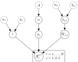
A α aλ bλ λj,r Wj,r φr bτ aτ τ β(r)j rj= 1= 1,, . . . , R2,3
Figure 3: Hierarchical shrinkage prior for the PARAFAC marginals. White circles with continuous border represent the parameters, white circles with dashed border represent fixed hyper-parameters.
π β(jr) Wj,r,φ, τ ∼ NIj(0, τ φrWj,r). (29f)
Concerning the covariance matrices for the noise term in eq. (16), the Kronecker structure does
not allow to separately identify the scale of the covariance matrices Un, thus requiring the
spec-ification of further restrictions. Wang and West (2009) and Dobra (2015) adopt independent
hyper-inverse Wishart prior distributions (Dawid and Lauritzen (1993)) for each Un, then
im-pose the identification restriction Un,11 = 1for n = 2, . . . , N. Instead, Hoff (2011) suggests to
introduce dependence between the Inverse Wishart prior distribution IW(νn, γΨn) of eachUn,
n= 1, . . . , N, via a hyper-parameter γ ∼ Ga(a, b) affecting the scale of each location matrix
pa-rameter. Finally, the hard constraintΣn=IIn (where Ik is the identity matrix of sizek), for all
but one n, implicitly imposes that the dependence structure within different modes is the same,
but there is no dependence between modes. To account for marginal dependence, it is possible to add a level of hierarchy by introducing a hyper-parameter in the spirit of Hoff (2011). Follow-ing Hoff (2011), we assume conditionally independent inverse Wishart prior distributions for the
covariance matrices of the error termEtand add a level of hierarchy via the hyper-parameterγ
which governs the scale of the covariance matrices:
π(γ)∼ Ga(aγ, bγ) (30a)
π(Σ1|γ)∼ IWI1(ν1, γΨ1) (30b)
π(Σ2|γ)∼ IWI2(ν2, γΨ2). (30c)
Defining the vector of all parameters as θ = {α,φ, τ,Λ,W,B,Σ1,Σ2}, with Λ = {λj,r : j =
1, . . . ,3, r = 1, . . . , R} and W={Wj,r :j= 1, . . . ,3, r= 1, . . . , R}, the joint prior distribution
is given by:
π(θ) =π(B|W,φ, τ)π(W|Λ)π(φ|α)π(τ|α)π(Λ)π(α)π(Σ1|γ)π(Σ2|γ)π(γ). (31)
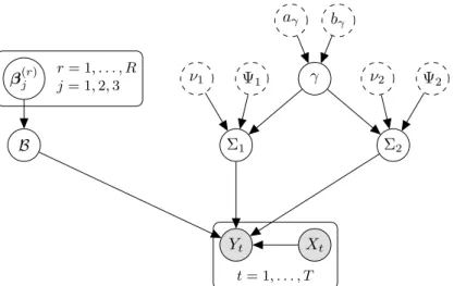
The directed acyclic graphs (DAG) of the hierarchical shrinkage prior on the PARAFAC marginals
ν1 Ψ1 γ ν2 Ψ2 aγ bγ Σ1 Σ2 β(r)j B Yt Xt r= 1, . . . , R j= 1,2,3 t= 1, . . . , T
Figure 4: Overall prior structure. Gray circles represent observable variables, white circles with continuous border represent the parameters, white circles with dashed border represent fixed hyper-parameters.
3.2 Posterior Computation
The likelihood function of the model in eq. (26) is given by:
L Y1, . . . , YT|θ = T Y t=1 (2π)−I12I2 |Σ2|− I1 2 |Σ1|− I2 2 exp −1 2Σ −1 2 (Yt− B ×3xt)0Σ1−1(Yt− B ×3xt) , (32)
where xt = vec (Xt). Since the posterior distribution is not tractable in closed form, we adopt
an MCMC procedure based on Gibbs sampling. The computations and technical details of
the derivation of the posterior distributions are given in Appendix D. As a consequence of the hierarchical structure of the prior, we can articulate the sampler in three main blocks:
I) sample the hyper-parameters of the global and component-level variance for the marginals, according to:
p(α,φ, τ|B,W) =p(α|B,W)p(φ, τ|α,B,W) (33)
(i) sample αfrom:
P α=αj |B,W = p(αj|B,W) P|A| l=1p(αl|B,W) , (34) where: p(α|B,W) =π(α) 1 M M|A| X i=1 ωi. (35)
(ii) sample independently the auxiliary variable ψr, for r= 1, . . . , R, from:
p(ψr|B,W, α)∝GiG α−I0 2,2bτ,2Cr (36) then, for r= 1, . . . , R: φr = PRψr l=1ψl . (37) 13
(iii) finally, sampleτ from: p(τ|B,W,φ)∝GiG aτ − RI0 2 ,2bτ,2 R X r=1 Cr φr . (38)
II) define Y = {Yt}Tt=1, then sample from the posterior of the hyper-parameters of the local
component of the variance of the marginals and the marginals themselves, as follows:
p β(jr), Wj,r, λj,r φ, τ,Y,Σ1,Σ2 =p λj,r|β(jr), φr, τ p wj,r,p|λj,r, φr, τ,β(jr) ·pβ(jr)|β−j(r),B−r, φr, τ,Y,Σ1,Σ2 (39)
(i) forj= 1,2,3 and r= 1, . . . , Rsample independently:
p λj,r|β(jr), φr, τ ∝ Ga aλ+Ij, bλ+ β (r) j 1 √ τ φr . (40)
(ii) for p= 1, . . . , Ij,j = 1,2,3and r= 1, . . . , Rsample:
pwj,r,p|λj,r, φr, τ,β(jr) ∝GiG 1 2, λ 2 j,r, βj,k(r)2 τ φr (41) (iii) defineβ(−jr)= n β(ir) :i6=j o
and B−r ={Bi :i6=r}, where Br=β(1r)◦. . .◦β(Nr). For
r = 1, . . . , Rsample the PARAFAC marginals from:
pβ(1r)|β−(r1),B−r, φr, τ,Y,Σ1,Σ2 ∝ NI1( ¯µβ 1, ¯ Σβ1) (42) p β(2r)|β−(r2),B−r, φr, τ,Y,Σ1,Σ2 ∝ NI2( ¯µβ2, ¯ Σβ2) (43) pβ(3r)|β(−r3),B−r, φr, τ,Y,Σ1,Σ2∝ NI3( ¯µβ 3, ¯ Σβ3). (44)
III) sample the covariance matrices from their posterior:
p(Σ1,Σ2, γ|B,Y) =p(Σ1|B,Y,Σ2, γ)p(Σ2|B,Y,Σ1, γ)p(γ|Σ1,Σ2) (45) (i) sample the row covariance matrix:
p(Σ1|B,Y,Σ2, γ)∝ IWI1(ν1+I1, γΨ1+S1) (46)
(ii) sample the column covariance matrix:
p(Σ2|B,Y,Σ1, γ)∝ IWI2(ν2+I2, γΨ2+S2). (47)
(iii) sample the scale hyper-parameter:
p(γ|Σ1,Σ2)∝ Ga ν1I1+ν2I2,tr Ψ1Σ−11+ Ψ2Σ−21 . (48) For improving the mixing of the algorithm, it is possible to substitute the draw from the full
conditional distributon of the global variance parameter τ or of the PARAFAC marginals with
4
Simulation Results
We report the results of a simulation study where we have tested the performance of the proposed
sampler on synthetic datasets of matrix-valued sequences{Yt, Xt}Tt=1, whereYt, Xthave different
size across simulations. The methods described in this paper can be rather computationally intensive, nevertheless thanks to the tensor decomposition we used allows the estimation to be carried out on a laptop. All the simulations were run on an Apple MacBookPro with a 3.1GHz Intel Core i7 processor, RAM 16GB, using MATLAB r2017b with the aid of the Tensor Toolbox
v.2.66, taking about 30h for the highest-dimensional case (i.e. I1 =I2 = 50).
For different sizes (I1 =I2) of the response and covariate matrices, we generated a
matrix-variate time series {Yt, Xt}Tt=1 by simulating each entry of Xt from:
xij,t−µ=αij(xij,t−1−µ) +ηij,t, ηij,t∼ N(0,1) (49)
and a matrix-variate time series {Yt}t according to:
Yt=B ×3vec (Xt) +Et, Et∼ NI1,I2(0,Σ1,II2). (50)
whereE[ηij,tηkl,v] = 0,E[ηij,tEv] = 0,∀(i, j)6= (k, l),∀t6=v, and αij ∼ U(−1,1). We randomly
draw B by using the PARAFAC representation in eq. (11), with rank R = 5 and marginals
sampled from the prior distribution in eq. (29f).
The response and covariate matrices in the simulated datasets have the following sizes:
(I) I1 =I2=I = 10, for T = 60;
(II) I1 =I2=I = 20, for T = 60;
(III) I1 =I2=I = 30, for T = 60;
(IV) I1 =I2=I = 40, for T = 60;
(V) I1 =I2=I = 50, for T = 60.
We initialized the Gibbs sampler by setting the PARAFAC marginalsβ(1r),β2(r),β(3r),r= 1, . . . , R
(withR= 5), with the output of a simulated annealing algorithm (see Appendix C) and run the
algorithm forN = 10000iterations. We present the results for the caseΣ2=II2. Since they are
similar, we omit the results for unconstrained Σ2, estimated with the Gibbs in Section 3.
6
Available at: http://www.sandia.gov/ tgkolda/TensorToolbox/index-2.6.html
I = 10 -10 -8 -6 -4 -2 0 2 -10 -8 -6 -4 -2 0 2 I = 20 -14 -12 -10 -8 -6 -4 -2 0 2 -15 -10 -5 0 I = 30 -16 -14 -12 -10 -8 -6 -4 -2 0 2 -16 -14 -12 -10 -8 -6 -4 -2 0 2 I = 40 200 400 600 800 1000 1200 1400 1600 200 400 600 800 1000 1200 1400 1600 -14 -12 -10 -8 -6 -4 -2 0 2 200 400 600 800 1000 1200 1400 1600 200 400 600 800 1000 1200 1400 1600 -18 -16 -14 -12 -10 -8 -6 -4 -2 0 2 I = 50 -16 -14 -12 -10 -8 -6 -4 -2 0 2 4 -18 -16 -14 -12 -10 -8 -6 -4 -2 0 2
Figure 5: Logarithm of the absolute value of the coefficient tensors: true B
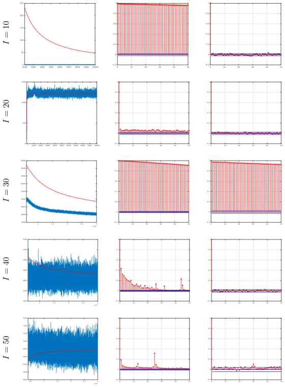
I = 10 I = 20 I = 30 I = 40 I = 50
Figure 6: MCMC output (left), autocorrelation function for the entire sample
(middle plot) and after burn-in (right plot) of the Frobenious norm of the
difference between the true and the estimated covariance matrix Σ1.
The results are reported in Figs. 5-6, for the different simulated datasets. Fig. 5 shows the good accuracy of the sampler in estimating the coefficient tensor, whose number of entries ranges
from 104 in the first to 504 in the last simulation setting. The estimation error is maily due to
the over-shrinking to zero of large signals. This well known drawback of global-local hierarchical prior distributions (e.g., see Carvalho et al. (2010)) is related to its sensitivity to the
hyper-parameters setting. Fig. 6 plots the MCMC output of the Frobenious norm (i.e. the L2 norm)
of the covariance matrix of the error term. After a graphical inspection of the trace plots (first 17
column) we chose a burn-in period of 2000 iterations. Due to autocorrelation in the sample
(second column plots) we applied thinning and selected every 10th iteration. In most of the
cases, after removing burn-in iterations and performing thinning, the autocorrelation wipes out. We refer the reader to Appendix F for additional details on the simulation experiments, such as trace plots and autocorrelation functions for tensor entries and individual hyper-parameters.
5
Application
5.1 Data description
As put forward by Schweitzer et al. (2009), the analysis of economic networks is one of the most recent and complex challenges that the econometric community is facing nowadays. We con-tribute to the econometric literature about complex networks by applying the proposed method-ology to the study of the temporal evolution of the international trade network (ITN). This economic network has been previously studied by several authors (e.g., see Hidalgo and Haus-mann (2009), Fagiolo et al. (2009), Kharrazi et al. (2017), Meyfroidt et al. (2010), Zhu et al. (2014), Squartini et al. (2011)), who have analysed its topological properties and identified its main communities. However, to the best of our knowledge, this is the first attempt to model the temporal evolution of the network as a whole.
The raw trade data come from the United Nations COMTRADE database, a publicly
avail-able resource7. The particular dataset we use is a subset of the whole COMTRADE database
and consists of yearly observations from 1998 to 2016 of total imports and exports between
I1 = I2 =I = 10countries. In order to remove possible sources of non-linearities in the data,
we use a logarithmic transform of the variables of interest. We thus consider the international trade network at each time stamp as one observation from a real-valued matrix-variate stochastic process. Fig. 7 shows the whole network sequence in our dataset.
5.2 Results
We estimate the model settingXt=Yt−1, thus obtaining a matrix-variate autoregressive model.
Each matrixYtis theI×I real-valued weighted adjacency matrix of the corresponding
interna-tional trade network in yeart, whose entry (i, j)contains the total exports of countryivis-à-vis
country j, in year t. The series {Yt}t, t = 1, . . . , T, has been standardized (over the temporal
dimension). We run the Gibbs sampler forN = 10,000iterations. The output is reported below.
-0.15 -0.1 -0.05 0 0.05 0.1 0.15 0.2 0 10 20 30 40 50 60 70 80 90 100 -10 -9 -8 -7 -6 -5 -4 -3 -2 -1 0
Figure 8: Left: Transpose of the mode-3 matricized estimated coefficient
tensor, Bˆ0(3). Middle: distribution of the estimated entries of Bˆ(3). Right:
logarithm of the modulus of the eigenvalues of Bˆ(3), in decreasing order.
7
(1998) (1999) (2000) (2001) (2002) CH AU DE DK FR GB IE JP SE US CH AU DE DK FR GB IE JP SE US CH AU DE DK FR GB IE JP SE US CH AU DE DK FR GB IE JP SE US CH AU DE DK FR GB IE JP SE US (2003) (2004) (2005) (2006) (2007) CH AU DE DK FR GB IE JP SE US CH AU DE DK FR GB IE JP SE US CH AU DE DK FR GB IE JP SE US CH AU DE DK FR GB IE JP SE US CH AU DE DK FR GB IE JP SE US (2008) (2009) (2010) (2011) (2012) CH AU DE DK FR GB IE JP SE US CH AU DE DK FR GB IE JP SE US CH AU DE DK FR GB IE JP SE US CH AU DE DK FR GB IE JP SE US CH AU DE DK FR GB IE JP SE US (2013) (2014) (2015) (2016) CH AU DE DK FR GB IE JP SE US CH AU DE DK FR GB IE JP SE US CH AU DE DK FR GB IE JP SE US CH AU DE DK FR GB IE JP SE US
Figure 7: Commercial trade network evolving over time from 1998 (top left)
to 2016 (bottom right). Nodes represent countries, red and blue colored
edges stand for exports and imports between two countries, respectively. Edge thickness represents the magnitude of the flow.
2 4 6 8 10 1 2 3 4 5 6 7 8 9 10 0 0.2 0.4 0.6 0.8 1 1.2 1.4 1.6 10002000300040005000600070008000 1.5 2 2.5 3 3.5 4 4.5 -0.2 0 0.2 0.4 0.6 0.8 1 0 10 20 30 40 50 2 4 6 8 10 1 2 3 4 5 6 7 8 9 10 -0.1 0 0.1 0.2 0.3 0.4 0.5 0.6 0.7 0.8 1000 2000 3000 4000 5000 6000 7000 8000 1.2 1.4 1.6 1.8 2 2.2 2.4 2.6 2.8 3 -0.2 0 0.2 0.4 0.6 0.8 1 0 10 20 30 40 50
Figure 9: Estimated covariance matrix of the noise term (first), posterior
distributions (second), MCMC output (third) and autocorrelation functions
(fourth) of the Frobenious norm of the covariance matrix of the noise term.
First row: Σ1,second row: Σ2.
The mod-3matricization of the estimated coefficient tensor is shown in the left panel of Fig. 8, each column corresponds to the effects of a lag one edge (horizontal axis) on all the contempo-raneous edges (vertical axis). Positive effects in red and negative effects in blue. Fig. 9 shows
the estimated covariance matrices of the noise term, that is Σˆ1,Σˆ2. As regards the estimated
coefficient tensor, we find that:
• the heterogeneity in the estimated coefficients points against parameter pooling
assump-tions;
• there are patterns, it look like there are groups of edges (bilateral trade flows) with mainly
positive (red) or negative (blue) effect on all the other edges. Maybe there are some
countries that play a key role for these flows;
• the distribution of the entries of the estimated coefficient tensor (middle panel) confirms
the evidence of heterogeneity. The distribution is right-skewed and leptokurtic with mode at zero, which is a consequence of the shrinkage of the estimated coefficient;
• in order to assess the stationarity of the model, we computed the eigenvalues of the
mode-3 matricization of the estimated coefficient tensor and the right panel of Fig. 8 plots the
logarithm of their modulus. All the eigenvalues are strictly lower than one in modulus, thus indicating that the process describing the evolution of the trade network is stationary. Moreover, as regards the estimated covariance matrices of the noise term (Fig. 9), we find that:
• in both cases the highest values correspond to individual variances, while the estimated
covariances are lower in magnitude and heterogeneous;
• there is evidence of heterogeneity in the dependence structure, since Σ1, which captures
the covariance between exporting countries (i.e., rows), differs from Σ2, which describes
the covariance between importing countries (i.e., columns);
• the dependence between exporting countries is higher on average than between importing
countries;
• for assessing the convergence of the MCMC chain, Fig. 9 shows the trace plot and
auto-correlation functions (without thinning) of the Frobenious norm of each estimated matrix. Both sets of plots show a good mixing of the chain.
5.3 Impulse response analysis
For understanding the role exerted by the various links of the network, Fig. 10, top panel, shows for each edge the sum of the corresponding positive and negative entries of the estimated coefficient tensor in red and blue, respectively. We find that edges’ impact tend to cluster, that is, those with high positive cumulated effects have very low negative cumulated effects and vice-versa. Thus, the bottom panel of Fig. 10 shows the sum of the absolute values of all corresponding entries of the estimated coefficient tensor, which can be interpreted as a measure of the importance of the edge in the network. Based on this statistic, we plot the position of the
10 most and least relevant edges in the network (in red and blue, respectively) in Fig 11. The
picture has a heterogeneous structure: first, no single country seems to exert a key role, neither as exporter nor as importer; second, the most and least relevant edges are evenly distributed between the exporting and the importing side.
We study the effects of the propagation of a shock on a single and a group of edges in the network by means of the impulse response function obtained as follows. Define the reverse of
the vectorization operator vec (·) by vecr (·) and let E˜ be a binary matrix of shocks such that
each non zero entry (i, j) of E˜ corresponds to a unitary shock on the edge (i, j). Then the
matrix-valued impulse response function is obtained from the recursion:
Y1=B ×3vec ˜ E = vecr B0(3)·vec ˜ E (51) Y2=B ×3vec vecr B0(3)·vec ˜ E ! = vecr B0(3)·B0(3)·vec ˜ E (52) = vecr [B0(3)]2·vec ˜ E , (53)
which, for the horizon h >0, generalizes to:
Yh= vecr [B0(3)]h·vec ˜ E . (54)
This equation shows that it is possible to study the joint effect that a contemporaneous shock on a subset of the edges of the network has on the whole network over time.
Fig. 12 and 13, respectively, plot the impulse response function of a unitary shock on the10
most relevant and the 10 least relevant edges (determined by ranking according to the sum of
the absolute values of the entries of the estimated coefficient tensor), for h = 1, . . . ,14 periods.
Figs. 14-15 show the effects of a unitary shock to the most and least influential edges, respectively. We find that:
• the effects are remarkably different: both the magnitude and the persistence of the impact
of a shock to the most relevant edges is significantly greater than that obtained by hitting the least relevant edges;
• with reference to figs. 14-15, as in the previous case, a shock to the most relevant edge
is more persistent than a shock on the least relevant and the magnitude is higher.
How-ever, compared to the effects of a shock on 10 edges, both persistence and magnitude are
remarkably lower;
• a shock to a single edge affects almost all the others because of the high degree of
inter-connection of the network, which is responsible for the propagation both in the space (i.e. cross-section) and over time.
Figure 10: Sum of positive entries (red,top), negative entries (blue,top) and of
absolute values of all entries (dark green,bottom) of the estimated coefficient
tensor (y-axis), per each edge (x-axis).
AU CH DE DK FR GB IE JP SE US AU CH DE DK FR GB IE JP SE US
Figure 11: Position in the network of the 10 most relevant (red) and least
relevant (blue) edges, according to the sum of the absolute values. Countries’
labels on both axes.
AUCHDEDK FRGB IE JP SEUS AU CH DE DK FR GB IE JP SE US 0 0.2 0.4 0.6 0.8 1 1.2 AUCHDEDK FRGB IE JP SEUS AU CH DE DK FR GB IE JP SE US AUCHDEDK FRGB IE JP SEUS AU CH DE DK FR GB IE JP SE US AUCHDEDK FRGB IE JP SEUS AU CH DE DK FR GB IE JP SE US AUCHDEDK FRGB IE JP SEUS AU CH DE DK FR GB IE JP SE US AUCHDEDK FRGB IE JP SEUS AU CH DE DK FR GB IE JP SE US AUCHDEDK FRGB IE JP SEUS AU CH DE DK FR GB IE JP SE US AUCHDEDK FRGB IE JP SEUS AU CH DE DK FR GB IE JP SE US AUCHDEDK FRGB IE JP SEUS AU CH DE DK FR GB IE JP SE US AUCHDEDK FRGB IE JP SEUS AU CH DE DK FR GB IE JP SE US AUCHDEDK FRGB IE JP SEUS AU CH DE DK FR GB IE JP SE US AUCHDEDK FRGB IE JP SEUS AU CH DE DK FR GB IE JP SE US AUCHDEDK FRGB IE JP SEUS AU CH DE DK FR GB IE JP SE US AUCHDEDK FRGB IE JP SEUS AU CH DE DK FR GB IE JP SE US
Figure 12: Impulse response forh= 1, . . . ,14periods. Unitary shock on the
10 most relevant edges (sum of absolute values of all coefficients). Countries’ labels on both axes.
AUCHDEDK FRGB IE JP SEUS AU CH DE DK FR GB IE JP SE US -0.5 -0.4 -0.3 -0.2 -0.1 0 AUCHDEDK FRGB IE JP SEUS AU CH DE DK FR GB IE JP SE US AUCHDEDK FRGB IE JP SEUS AU CH DE DK FR GB IE JP SE US AUCHDEDK FRGB IE JP SEUS AU CH DE DK FR GB IE JP SE US AUCHDEDK FRGB IE JP SEUS AU CH DE DK FR GB IE JP SE US AUCHDEDK FRGB IE JP SEUS AU CH DE DK FR GB IE JP SE US AUCHDEDK FRGB IE JP SEUS AU CH DE DK FR GB IE JP SE US AUCHDEDK FRGB IE JP SEUS AU CH DE DK FR GB IE JP SE US AUCHDEDK FRGB IE JP SEUS AU CH DE DK FR GB IE JP SE US AUCHDEDK FRGB IE JP SEUS AU CH DE DK FR GB IE JP SE US AUCHDEDK FRGB IE JP SEUS AU CH DE DK FR GB IE JP SE US AUCHDEDK FRGB IE JP SEUS AU CH DE DK FR GB IE JP SE US AUCHDEDK FRGB IE JP SEUS AU CH DE DK FR GB IE JP SE US AUCHDEDK FRGB IE JP SEUS AU CH DE DK FR GB IE JP SE US
Figure 13: Impulse response forh= 1, . . . ,14periods. Unitary shock on the
10 least relevant edges (sum of absolute values of all coefficients). Countries’ labels on both axes.
AUCHDEDK FRGB IE JP SEUS AU CH DE DK FR GB IE JP SE US 0 0.2 0.4 0.6 0.8 1 1.2 AUCHDEDK FRGB IE JP SEUS AU CH DE DK FR GB IE JP SE US AUCHDEDK FRGB IE JP SEUS AU CH DE DK FR GB IE JP SE US AUCHDEDK FRGB IE JP SEUS AU CH DE DK FR GB IE JP SE US AUCHDEDK FRGB IE JP SEUS AU CH DE DK FR GB IE JP SE US AUCHDEDK FRGB IE JP SEUS AU CH DE DK FR GB IE JP SE US AUCHDEDK FRGB IE JP SEUS AU CH DE DK FR GB IE JP SE US AUCHDEDK FRGB IE JP SEUS AU CH DE DK FR GB IE JP SE US AUCHDEDK FRGB IE JP SEUS AU CH DE DK FR GB IE JP SE US AUCHDEDK FRGB IE JP SEUS AU CH DE DK FR GB IE JP SE US AUCHDEDK FRGB IE JP SEUS AU CH DE DK FR GB IE JP SE US AUCHDEDK FRGB IE JP SEUS AU CH DE DK FR GB IE JP SE US AUCHDEDK FRGB IE JP SEUS AU CH DE DK FR GB IE JP SE US AUCHDEDK FRGB IE JP SEUS AU CH DE DK FR GB IE JP SE US
Figure 14: Impulse response forh= 1, . . . ,14periods. Unitary shock on the
most relevant edge (sum of absolute values of all coefficients). Countries’ labels on both axes.
AUCHDEDK FRGB IE JP SEUS AU CH DE DK FR GB IE JP SE US -0.5 -0.4 -0.3 -0.2 -0.1 0 AUCHDEDK FRGB IE JP SEUS AU CH DE DK FR GB IE JP SE US AUCHDEDK FRGB IE JP SEUS AU CH DE DK FR GB IE JP SE US AUCHDEDK FRGB IE JP SEUS AU CH DE DK FR GB IE JP SE US AUCHDEDK FRGB IE JP SEUS AU CH DE DK FR GB IE JP SE US AUCHDEDK FRGB IE JP SEUS AU CH DE DK FR GB IE JP SE US AUCHDEDK FRGB IE JP SEUS AU CH DE DK FR GB IE JP SE US AUCHDEDK FRGB IE JP SEUS AU CH DE DK FR GB IE JP SE US AUCHDEDK FRGB IE JP SEUS AU CH DE DK FR GB IE JP SE US AUCHDEDK FRGB IE JP SEUS AU CH DE DK FR GB IE JP SE US AUCHDEDK FRGB IE JP SEUS AU CH DE DK FR GB IE JP SE US AUCHDEDK FRGB IE JP SEUS AU CH DE DK FR GB IE JP SE US AUCHDEDK FRGB IE JP SEUS AU CH DE DK FR GB IE JP SE US AUCHDEDK FRGB IE JP SEUS AU CH DE DK FR GB IE JP SE US
Figure 15: Impulse response for h = 1, . . . ,14 periods. Unitary shock on
the least relevant edge (sum of absolute values of all coefficients). Countries’ labels on both axes.
6
Conclusions
We defined a new statistical framework for dynamic tensor regression. It is a generalisation of many models frequently used in time series analysis, such as VAR, panel VAR, SUR and matrix
regression models. The PARAFAC decomposition of the tensor of regression coefficients allows to reduce the dimension of the parameter space but also permits to choose flexible multivariate prior distributions, instead of multidimensional ones. Overall, this allows to encompass sparsity beliefs and to design efficient algorithm for posterior inference.
We tested the Gibbs sampler algorithm on synthetic matrix-variate datasets with matrices of different sizes, obtaining good results in terms of both the estimation of the true value of the parameter and the efficiency.
The proposed methodology has been applied to the analysis of temporal evolution of a subset of the international trade networks. We found evidence of (i) wide heterogeneity in the sign and magnitude of the estimated coefficients; (ii) stationarity of the network process.
Acknowledgements
This research has benefited from the use of the Scientific Computation System of Ca’ Foscari University of Venice (SCSCF) for the computational for the implementation of the estimation procedure.
References
Abraham, R., Marsden, J. E., and Ratiu, T. (2012).Manifolds, tensor analysis, and applications.
Springer Science & Business Media.
Adler, R., Bazin, M., and Schiffer, M. (1975). Introduction to general relativity. McGraw-Hill
New York.
Aldasoro, I. and Alves, I. (2016). Multiplex interbank networks and systemic importance: an
application to European data. Journal of Financial Stability.
Anacleto, O. and Queen, C. (2017). Dynamic chain graph models for time series network data.
Bayesian Analysis, 12(2):491–509.
Arashi, M. (2017). Some theoretical results on tensor elliptical distribution. arXiv preprint
arXiv:1709.00801.
Aris, R. (2012).Vectors, tensors and the basic equations of fluid mechanics. Courier Corporation.
Balazsi, L., Matyas, L., and Wansbeek, T. (2015). The estimation of multidimensional fixed
effects panel data models. Econometric Reviews, pages 1–23.
Barrat, A., Fernandez, B., Lin, K. K., and Young, L.-S. (2013). Modeling temporal networks
using random itineraries. Physical Review Letters, 110(15).
Bhattacharya, A., Pati, D., Pillai, N. S., and Dunson, D. B. (2015). Dirichlet-Laplace priors for
optimal shrinkage. Journal of the American Statistical Association, 110(512):1479–1490.
Canova, F. and Ciccarelli, M. (2004). Forecasting and turning point predictions in a Bayesian
panel VAR model. Journal of Econometrics, 120(2):327–359.
Canova, F. and Ciccarelli, M. (2009). Estimating multicountry VAR models. International
Canova, F. and Ciccarelli, M. (2013). Panel vector autoregressive models: a survey, volume 32, chapter 12, pages 205–246. Emerald Group Publishing Limited, VAR models in macroeco-nomics – new developments and applications: essays in honor of Christopher A. Sims edition. Canova, F., Ciccarelli, M., and Ortega, E. (2007). Similarities and convergence in G-7 cycles.
Journal of Monetary Economics, 54(3):850–878.
Canova, F., Ciccarelli, M., and Ortega, E. (2012). Do institutional changes affect business cycles?
evidence from Europe. Journal of Economic Dynamics and Control, 36(10):1520–1533.
Carriero, A., Kapetanios, G., and Marcellino, M. (2016). Structural analysis with multivariate
autoregressive index models. Journal of Econometrics, 192(2):332–348.
Carroll, J. D. and Chang, J.-J. (1970). Analysis of individual differences in multidimensional
scaling via an N-way generalization of “Eckart-Young” decomposition.Psychometrica, 35:283–
319.
Carvalho, C. M., Massam, H., and West, M. (2007). Simulation of hyper-inverse Wishart
distri-butions in graphical models. Biometrika, 94(3):647–659.
Carvalho, C. M., Polson, N. G., and Scott, J. G. (2010). The horseshoe estimator for sparse
signals. Biometrika, 97(2):465–480.
Carvalho, C. M. and West, M. (2007). Dynamic matrix-variate graphical models. Bayesian
Analysis, 2(1):69–97.
Cichocki, A. (2014). Era of Big data processing: a new approach via tensor networks and tensor
decompositions. arXiv preprint arXiv:1403.2048.
Cichocki, A., Zdunek, R., Phan, A. H., and Amari, S.-i. (2009). Nonnegative matrix and tensor
factorizations: applications to exploratory multi-way data analysis and blind source separation. John Wiley & Sons.
Cook, R. D., Li, B., and Chiaromonte, F. (2010). Envelope models for parsimonious and efficient
multivariate linear regression. Statistica Sinica, 20:927–960.
Dawid, A. P. and Lauritzen, S. L. (1993). Hyper Markov laws in the statistical analysis of
decomposable graphical models. The Annals of Statistics, 21(3):1272–1317.
Ding, S. and Cook, R. D. (2016). Matrix-variate regressions and envelope models. arXiv preprint
arXiv:1605.01485.
Dobra, A. (2015). Handbook of Spatial Epidemiology, chapter Graphical Modeling of Spatial
Health Data. Chapman & Hall /CRC, first edition.
Durante, D. and Dunson, D. B. (2014). Nonparametric Bayesian dynamic modelling of relational
data. Biometrika, 101(4):883–898.
Eckart, C. and Young, G. (1936). The approximation of one matrix by another of lower rank.
Psychometrika, 1(3):211–218.
Engle, R. F. and Granger, C. W. (1987). Co-integration and error correction: representation,
estimation, and testing. Econometrica, pages 251–276.
Fagiolo, G., Reyes, J., and Schiavo, S. (2009). World-trade web: topological properties, dynamics,
and evolution. Physical Review E, 79(3):036115.
George, E. I. and McCulloch, R. E. (1997). Approaches for Bayesian variable selection.Statistica Sinica, 7:339–373.
Guhaniyogi, R., Qamar, S., and Dunson, D. B. (2017). Bayesian tensor regression. Journal of
Machine Learning Research, 18(79):1–31.
Gupta, A. K. and Nagar, D. K. (1999). Matrix variate distributions. CRC Press.
Hackbusch, W. (2012).Tensor spaces and numerical tensor calculus. Springer Science & Business
Media.
Harrison, J. and West, M. (1999). Bayesian forecasting & dynamic models. Springer.
Harshman, R. A. (1970). Foundations of the PARAFAC procedure: models and conditions for
an “explanatory” multi-modal factor analysis. UCLA Working Papers in Phonetics, 16, 1- 84.
Hidalgo, C. A. and Hausmann, R. (2009). The building blocks of economic complexity.
Proceed-ings of the national academy of sciences, 106(26):10570–10575.
Hoff, P. D. (2011). Separable covariance arrays via the Tucker product, with applications to
multivariate relational data. Bayesian Analysis, 6(2):179–196.
Hoff, P. D. (2015). Multilinear tensor regression for longitudinal relational data. The Annals of
Applied Statistics, 9(3):1169–1193.
Holme, P. and Saramäki, J. (2012). Temporal networks. Physics Reports, 519(3):97–125.
Holme, P. and Saramäki, J. (2013). Temporal networks. Springer.
Hung, H. and Wang, C.-C. (2013). Matrix variate logistic regression model with application to
EEG data. Biostatistics, 14(1):189–202.
Imaizumi, M. and Hayashi, K. (2016). Doubly decomposing nonparametric tensor regression. In
International Conference on Machine Learning, pages 727–736.
Ishwaran, H. and Rao, J. S. (2005). Spike and slab variable selection: frequentist and Bayesian
strategies. Annals of Statistics, pages 730–773.
Kharrazi, A., Rovenskaya, E., and Fath, B. D. (2017). Network structure impacts global
com-modity trade growth and resilience. PloS one, 12(2):e0171184.
Kiers, H. A. (2000). Towards a standardized notation and terminology in multiway analysis.
Journal of Chameometrics, 14(3):105–122.
Kolda, T. G. (2006). Multilinear operators for higher-order decompositions. Technical report, Sandia National Laboratories.
Kolda, T. G. and Bader, B. W. (2009). Tensor decompositions and applications. SIAM Review,
51(3):455–500.
Kostakos, V. (2009). Temporal graphs. Physica A: Statistical Mechanics and its Applications,
388(6):1007–1023.
Kroonenberg, P. M. (2008). Applied multiway data analysis. John Wiley & Sons.
Kruijer, W., Rousseau, J., and Van Der Vaart, A. (2010). Adaptive Bayesian density estimation
Lee, N. and Cichocki, A. (2016). Fundamental tensor operations for large-scale data analysis in
tensor train formats. arXiv preprint arXiv:1405.7786.
Li, L. and Zhang, X. (2017). Parsimonious tensor response regression. Journal of the American
Statistical Association, 112(519):1131–1146.
Lovelock, D. and Rund, H. (1989).Tensors, differential forms, and variational principles. Courier
Corporation.
Malvern, L. E. (1986). Introduction to the mechanics of a continuous medium. Englewood.
Manceur, A. M. and Dutilleul, P. (2013). Maximum likelihood estimation for the tensor normal
distribution: algorithm, minimum sample size, and empirical bias and dispersion. Journal of
Computational and Applied Mathematics, 239:37–49.
Meyfroidt, P., Rudel, T. K., and Lambin, E. F. (2010). Forest transitions, trade, and the global
displacement of land use. Proceedings of the National Academy of Sciences, 107(49):20917–
20922.
Mitchell, T. J. and Beauchamp, J. J. (1988). Bayesian variable selection in linear regression.
Journal of the American Statistical Association, 83(404):1023–1032.
Neal, R. M. (2011). MCMC using Hamiltonian dynamics. In Brooks, S., Gelman, A., Galin,
J. L., and Meng, X.-L., editors,Handbook of Markov Chain Monte Carlo, chapter 5. Chapman
& Hall /CRC.
Ohlson, M., Ahmad, M. R., and Von Rosen, D. (2013). The multilinear normal distribution:
introduction and some basic properties. Journal of Multivariate Analysis, 113:37–47.
Pan, R. (2014). Tensor transpose and its properties. arXiv preprint arXiv:1411.1503.
Park, T. and Casella, G. (2008). The Bayesian lasso. Journal of the American Statistical
Asso-ciation, 103(482):681–686.
Poledna, S., Molina-Borboa, J. L., Martínez-Jaramillo, S., Van Der Leij, M., and Thurner, S. (2015). The multi-layer network nature of systemic risk and its implications for the costs of
financial crises. Journal of Financial Stability, 20:70–81.
Press, W. H., Teukolsky, S. A., Vetterling, W. T., and Flannery, B. P. (2007). Numerical recipes:
the art of scientic computing. Cambridge University Press.
Ritter, C. and Tanner, M. A. (1992). Facilitating the Gibbs sampler: the Gibbs stopper and the
griddy-Gibbs sampler. Journal of the American Statistical Association, 87(419):861–868.
Robert, C. P. and Casella, G. (2004). Monte Carlo statistical methods. Springer.
Schotman, P. and Van Dijk, H. K. (1991). A Bayesian analysis of the unit root in real exchange
rates. Journal of Econometrics, 49(1-2):195–238.
Schweitzer, F., Fagiolo, G., Sornette, D., Vega-Redondo, F., Vespignani, A., and White, D. R.
(2009). Economic networks: the new challenges. Science, 325(5939):422–425.
Sims, C. A. and Zha, T. (1998). Bayesian methods for dynamic multivariate models.International
Economic Review, 39(4):949–968.